Chapter 11
Applications of EBMs: Optimal Estimation
11.1 Introduction
An estimator is an algorithm making use of an observation or combination of observations in order to provide a useful estimate of some system parameter such as the global average temperature. In order to conduct such a procedure, we have to make a statistical model of our process. Once we have a statistical model in place, we can examine it and the estimation procedure to learn several things about the underlying system parameter. Usually, the estimator is a random variable that has some probability distribution (pdf) due to errors in the measurement process or perhaps sampling error. The following are some questions of interest: (i) does the mean of the pdf of the estimator coincide with the actual value of the system parameter? If it does, we say the estimator is unbiased. (ii) What is the variance of the estimator? The square root of this variance is the standard deviation or root mean square error or RMS error.
EBMs can be of service in some estimation problems. The usefulness of an EBM for a particular application comes in two forms:
- 1. Many estimation problems can be evaluated with the assistance of general circulation model (GCM) simulations. In this chapter, we use the EBM to show how a few of these work in the simpler context. In many cases with the EBM, we are able to solve the problem analytically or nearly so. This puts aside the issue of whether the more realistic model actually has a solution or whether it is over-fitted, and so on. In this application, we can focus on the estimation process from its beginning to its end without letting the details or mathematical transgressions cloud the picture. The main point is the understanding of the estimation process in a simple and more heuristic context. It might be that the lessons learned can be applied with much more complicated models.
- 2. There are some estimation problems where it might not be feasible to solve the problem in the more complicated models because of lack of computing or data resources. For example, how many fully coupled GCMs have a 10 000 year control run with which to assess the low-frequency statistical parameters of natural variability? How can our intuition about such problems be enhanced? To paraphrase a statement by John Maynard Keynes, “it might be better to have a rough idea of the truth than a very precise [or satisfying] answer which is wrong.”
In a typical case, there may be many unbiased estimators for a given problem, often combining lots of measurements, such as areal or temporal averages. Think of the estimate of the global average temperature. We might take gauge (point) measurements from a number of different stations or perhaps other observing systems (e.g., satellites). We suspect that if we simply average the data, then these averages might form an unbiased estimate of the global average temperature. We might ask whether a straight arithmetic average is actually the best unbiased estimator in terms of its RMS error. Perhaps some nonuniform weighting would improve the estimate. This general class of problems is the subject of this chapter. We will apply the method with the help of the EBM to two different examples: Section 11.3 on estimating the global average temperature; Section 11.4 on detecting faint deterministic signals (such as the greenhouse warming or episodic cooling by volcanic dust veils) in the climate system. We start with a simple problem involving two imperfect observations of a heat reservoir.
11.2 Independent Estimators
Consider estimating the temperature of a reservoir with two devices. Let the estimators ![]() and
and ![]() be unbiased; that is,
be unbiased; that is, ![]() where
where ![]() is the true temperature, and
is the true temperature, and ![]() means ensemble average.
means ensemble average.
The individual estimators are assumed to be of the form ![]() ; where the errors
; where the errors ![]() are assumed to be random variables taking on different values in each realization of the measurement process. The errors or noise are assumed to have mean zero when considered over a large number of trials:
are assumed to be random variables taking on different values in each realization of the measurement process. The errors or noise are assumed to have mean zero when considered over a large number of trials: ![]() , and the covariances of the errors are given by
, and the covariances of the errors are given by ![]() . The previous expression states that the errors of the separate devices are assumed to be uncorrelated and that their individual variances are given by
. The previous expression states that the errors of the separate devices are assumed to be uncorrelated and that their individual variances are given by ![]() and
and ![]() . We assume that these characteristics of the errors are known beforehand. Our task is to take one realization of the measurement process and obtain an optimal estimate of the true reservoir temperature. We wish to make maximal use of the data collected from each device in an appropriate linear combination. The question is, what is the appropriate weighting to assign to each measurement? We form the estimate
. We assume that these characteristics of the errors are known beforehand. Our task is to take one realization of the measurement process and obtain an optimal estimate of the true reservoir temperature. We wish to make maximal use of the data collected from each device in an appropriate linear combination. The question is, what is the appropriate weighting to assign to each measurement? We form the estimate
where ![]() is a weight to be adjusted to make the mean square error (MSE) the minimum. The estimator
is a weight to be adjusted to make the mean square error (MSE) the minimum. The estimator ![]() is clearly unbiased if the individual estimators are. We can form the MSE for the measurement as
is clearly unbiased if the individual estimators are. We can form the MSE for the measurement as
The latter is a quadratic in ![]() and is shown in Figure 11.1 for a choice of
and is shown in Figure 11.1 for a choice of ![]() . The point of this figure is that the MSE is rather insensitive to the choice of
. The point of this figure is that the MSE is rather insensitive to the choice of ![]() so long as it is near its optimum value. This is an important point to be stressed later in the climate signal detection exercises.
so long as it is near its optimum value. This is an important point to be stressed later in the climate signal detection exercises.
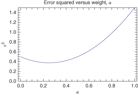
Figure 11.1 Error squared  versus weighting
  for two unbiased estimators.
The minimum of the quadratic above is easily found, and it yields the familiar and very important result:

where

The result is easily generalized to include ![]() independent unbiased estimators:
independent unbiased estimators:

and

An interesting way of expressing these last results is
with the column vector ![]() and
and

This last form gives us a convenient way of viewing the optimal estimation procedure in the form of an optimal filter of the raw data. The filter loads each observation with a weight inversely proportional to its individual error variance. The factor ![]() assures the normalization necessary for unbiasedness.
assures the normalization necessary for unbiasedness.
After some algebra, it can be shown that the optimal error variance is just

This shows that adding another device always improves the signal-to-noise ratio indicator no matter how poor its quality.
The derivation presented above required that the individual errors be uncorrelated with one another. If this were not so, the coordinate axes could simply be rotated to the principal axes of the error or noise covariance matrix. Then the entire formalism goes through as before except in the rotated coordinate system. In climatology, this is the transformation to the empirical orthogonal function (EOF) basis set, which we will return to in later sections.
In two dimensions, this is easily spelled out explicitly. Let the covariance matrix of the noise be given by
Taking the noise to be distributed bivariate normally, the contours of equal probability of occurrence of pairs of values of ![]() are given by (see Thiébaux, 1994):
are given by (see Thiébaux, 1994):

which is an ellipse in the ![]() plane. In this two-dimensional case, we can find an angle
plane. In this two-dimensional case, we can find an angle ![]() to rotate the coordinate axes through, such that the principal axes of the ellipse coincide with new coordinate axes
to rotate the coordinate axes through, such that the principal axes of the ellipse coincide with new coordinate axes ![]() . In the new coordinate system,
. In the new coordinate system, ![]() and
and ![]() are uncorrelated. In the case of
are uncorrelated. In the case of ![]() dimensions, the figure is an ellipsoid in the
dimensions, the figure is an ellipsoid in the ![]() -dimensional space and a simple length-preserving rotation can also be used to find the appropriate coordinate system. This rotation of the coordinate axes is familiar in data analysis as the transformation from spatial coordinates to the EOF basis set.
-dimensional space and a simple length-preserving rotation can also be used to find the appropriate coordinate system. This rotation of the coordinate axes is familiar in data analysis as the transformation from spatial coordinates to the EOF basis set.
The simple derivation of optimal weighting of independent estimators is familiar to many researchers. The result is very intuitive. We simply weight each estimator inversely according to its individual error variance.
11.3 Estimating Global Average Temperature
We will follow the method of Shen et al. (1994). The global average ![]() changes over time and it is smoothed over an interval
changes over time and it is smoothed over an interval ![]() centered at
centered at ![]() (it is a running average):
(it is a running average):

where ![]() refers to solid angle,
refers to solid angle, ![]() is a unit vector originating at the Earth's center and pointing to a location on the sphere, and
is a unit vector originating at the Earth's center and pointing to a location on the sphere, and

An anomaly at point ![]() is defined by
is defined by
and
and by definition, ![]() .
.
The global average temperature at time ![]() can be estimated for a given fixed network of stations
can be estimated for a given fixed network of stations ![]() :
:

and to ensure unbiasedness:

Our estimator is

where

and the MSE is given by
After multiplying the factors together,

and we have introduced the temporally smoothed covariance
To choose the optimal weighting coefficients, we need to use the method of Lagrange multipliers (e.g., Arfken and Weber, 2005). We minimize the function

where ![]() is a Lagrange multiplier.
is a Lagrange multiplier.
Next, we take partial derivatives

and
After inserting the expression for ![]() and rearranging, we find
and rearranging, we find

Our result is similar to the ![]() thermometer case of the last section. The problem here is that the temperatures at one location
thermometer case of the last section. The problem here is that the temperatures at one location ![]() and another
and another ![]() are correlated. To proceed, we need to know how to find variables that are not correlated. Thus the next section introduces EOFs.
are correlated. To proceed, we need to know how to find variables that are not correlated. Thus the next section introduces EOFs.
11.3.1 Karhunen–Loève Functions and Empirical Orthogonal Functions
We begin by noting that ![]() is a real symmetric function.1 Such functions play an important role in mathematical analysis. Consider, for example, the kernel of the integral in the eigenvalue problem2
is a real symmetric function.1 Such functions play an important role in mathematical analysis. Consider, for example, the kernel of the integral in the eigenvalue problem2
:

This equation is in the form of a Stürm–Liouville system (introduced in Chapter 7). The functions ![]() are the eigenfunctions for integer index
are the eigenfunctions for integer index ![]() and the
and the ![]() are the (real and positive) eigenvalues. Properties of Stürm–Liouville systems can be found in most books on mathematical methods for physicists and engineers (e.g., Arfken and Weber, 2005 and later editions). Additional properties include the orthogonality relation:
are the (real and positive) eigenvalues. Properties of Stürm–Liouville systems can be found in most books on mathematical methods for physicists and engineers (e.g., Arfken and Weber, 2005 and later editions). Additional properties include the orthogonality relation:

and the completeness relation:

The first of these tells us how to expand any reasonably well-behaved function3 on the sphere into these basis functions. The functions which are the eigenfunctions of the covariance kernel (11.28) are called the Karhunen–Loève functions (K-LFs). They form a convenient basis set into which many useful decompositions might be derived.
Consider developing the function ![]() into a series of these basis functions:
into a series of these basis functions:

The coefficients ![]() can be calculated from (11.29):
can be calculated from (11.29):

The completeness relation (11.30) assures that any well-behaved function on the sphere can be represented in the series.
Using these relations, we find that a function such as ![]() can be represented as
can be represented as

We can insert this last expression into (11.22) to obtain a matrix equation for the MSE, ![]() . Inspection of the result reveals that the problem can be cast into the form of a filter through which data in the form of correlation information can be entered. Shen et al. (1994) proceed by expanding each EOF,
. Inspection of the result reveals that the problem can be cast into the form of a filter through which data in the form of correlation information can be entered. Shen et al. (1994) proceed by expanding each EOF, ![]() , into a spherical harmonic4 series:
, into a spherical harmonic4 series:

where ![]() is a truncation level, typically set at spherical harmonic degree 11 or 15 in the experiments to be described.
is a truncation level, typically set at spherical harmonic degree 11 or 15 in the experiments to be described.
Let us now ask why optimal weighting helps. The key is the understanding of how the annual averaged surface temperature data are correlated from one location to another. This was examined in an important paper by Hansen and Lebedeff (1987). Figure 11.2 shows scatter diagrams of the correlation of the annual averaged surface temperatures in different latitude belts (the figure concentrates on the polar and mid-latitude belts; tropical spatial autocorrelations are not well defined, but in general are much longer). The correlations (on the average) fall off with separation distance to a level 1/e at about 1500 km.5
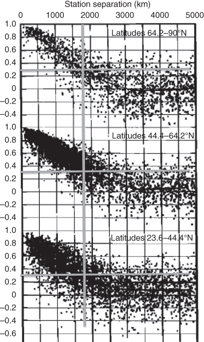
Figure 11.2 Spatial autocorrelation diagrams for annually averaged temperatures at stations separated by distances  . The solid lines are averages of the scattered points. The vertical and horizontal gray lines indicate the 1/e point and their values on the abscissa. Note that in the polar and mid-latitudes, the correlation lengths are about 1500 km.
(Hansen and Lebedeff (1987). © American Meteorological Society. Used with permission.)
The tropical temperatures do not follow this scheme. The reason is that in polar and mid-latitudes, the weather with autocorrelation times of the order of a few days drives the surface temperature field, which, for large scales, has an autocorrelation time of the order of weeks to a month over land and much longer over ocean. The conditions are right for the Langevin approximation used in Chapter 9. However, in the tropics, there is no weather noise and the dynamics smear out heat very quickly via direct circulations rather than in a kind of thermal diffusion.
We follow Shen et al. (1994) here to show that a relatively small number of gauges or sites (![]() ) are needed to achieve pretty good accuracy for estimating the global average temperature. Figure 11.3 shows the MSE for several gauge configurations:
) are needed to achieve pretty good accuracy for estimating the global average temperature. Figure 11.3 shows the MSE for several gauge configurations: ![]() , a 63 station well-dispersed gauge network used by Angell and Korshover (1983); and finally a
, a 63 station well-dispersed gauge network used by Angell and Korshover (1983); and finally a ![]() array. The EOFs (or K–LFs) were computed as indicated above using a spherical harmonic basis truncated at degree 11 using the data itself, and using the noise-forced 2-D model of Chapter 9. Figure 11.3 shows a graph of the MSE versus the number of EOF modes retained (
array. The EOFs (or K–LFs) were computed as indicated above using a spherical harmonic basis truncated at degree 11 using the data itself, and using the noise-forced 2-D model of Chapter 9. Figure 11.3 shows a graph of the MSE versus the number of EOF modes retained (![]() ) (the number of terms retained in (11.33)). This latter determines the dimension of the matrix problem. Note in the figure that the MSE levels off at a particular value of
) (the number of terms retained in (11.33)). This latter determines the dimension of the matrix problem. Note in the figure that the MSE levels off at a particular value of ![]() for each network configuration. Coarser networks require more modes than dense networks.
for each network configuration. Coarser networks require more modes than dense networks.

Figure 11.3 The mean squared error for estimation of the global average temperature as a function of the total number of spherical harmonic modes retained.
(Shen et al. (1994). © American Meteorological Society. Used with permission.)
To be complete, we must mention that the Shen et al. (1994) paper implicitly assumes that there is no power beyond the truncation level of the spherical harmonic expansion in the data. This is not quite true. But given the snugness of the fit in the figures, this might not be a bad approximation when the data are smoothed by time averaging (Figures 11.4 and 11.5).

Figure 11.4 Plots of the temperature estimate based on only 16 geometrically symmetrically located gauges (dashed line) together with the best estimate of the data from the UK CRU (Climate Research Unit) data set. The EOFs used in the optical weighting were based on the UK data. (a) Uniform weighting. (b) Optimal weighting.
(Shen et al. (1994). © American Meteorological Society. Used with permission.)
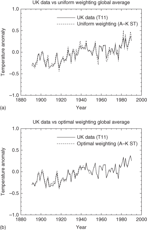
Figure 11.5 Similar to Figure 11.4 except for the 63 well-dispersed Angell–Korshover network. Note that the agreement is nearly perfect for the optimal weighting case.
(Shen et al. (1994). © American Meteorological Society. Used with permission.)
11.3.2 Relationship with EBMs
So what does this have to do with EBMs? The answer lies in the functional form of the spatial autocorrelation functions in Figure 11.2. We can compare with Figure 11.6, where the annually averaged data are from Siberia. The autocorrelation length in the latter figure is about 50% larger than in Figure 11.2. Both are based on annually averaged data. The reason for the longer autocorrelation length is that the latter figure is over a land mass, while the data from Hansen and Lebedeff are mixed over land and ocean. Ocean correlation lengths for annually averaged data are shown in Figures 9.8 and 9.9. From Figure 11.7, we can see that over land, where ![]() , the autocorrelation length
, the autocorrelation length ![]() , whereas over ocean, where
, whereas over ocean, where ![]() , and thus
, and thus ![]() . Hence, the autocorrelation length for all-land areas is large, while that over ocean is smaller, as suggested in both data and models of Figures 9.8 and 9.9.
. Hence, the autocorrelation length for all-land areas is large, while that over ocean is smaller, as suggested in both data and models of Figures 9.8 and 9.9.

Figure 11.6 Scatter diagram of spatial autocorrelation data from eastern Siberia. The data were annually averaged. The solid curve is based on the well-known model form  , where
  is the separation of stations in kilometers,
  is the modified Bessel function of the second kind and of degree unity (see Arfken and Weber, 2005), and the broken line is the average over the sample estimates.
(North et al. (2011). © American Meteorological Society. Used with permission.)
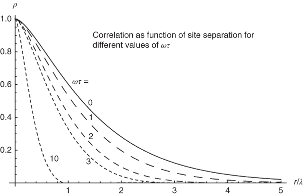
Figure 11.7 Theoretical (noise-forced EBM-based) spatial autocorrelation for different angular frequencies  . The relaxation time for the surface is
  (typically, a few years for a mixed-layer model) and
  is the characteristic length scale for
  . Over land, the characteristic length (
 ) is roughly twice the low-frequency limit over ocean (
 ).
).
(North et al. (2011). © American Meteorological Society. Used with permission.)
11.4 Deterministic Signals in the Climate System
The problem of detecting climate signals in the noisy background was first advanced by Hasselmann (1979), but also see Hasselmann (1993 1997). In this section, we take on the problem of detecting a faint signal in the noisy background of the climate system using a two-dimensional EBM. By signal, we mean a deterministic pattern in space–time—a response to a forced energy imbalance. The noise here is the natural variability as in our noise-forced EBMs of Chapter 9 or the natural variability in a GCM simulation. The statistical model we have in mind is that the data are a linear sum of signal and noise:
This would be true in the EBM world of a linear-sampled diffusive model driven by stationary random noise. It appears to be true also for large GCMs if ![]() is small enough. We have included a coefficient
is small enough. We have included a coefficient ![]() in front of the signal because we usually want to estimate the strength of the signal. In many applications, we know the space–time shape of the signal, but we do not know how strong it is. Often, the strength of such a signal depends on feedback factors that are only poorly known. We begin with a single signal and its characterization. To begin our discussion consider a sinusoidal wave in one dimension:
in front of the signal because we usually want to estimate the strength of the signal. In many applications, we know the space–time shape of the signal, but we do not know how strong it is. Often, the strength of such a signal depends on feedback factors that are only poorly known. We begin with a single signal and its characterization. To begin our discussion consider a sinusoidal wave in one dimension:
The coefficients ![]() and
and ![]() determine the amplitude and phase of the wave. We can characterize the signal as a vector in a two-dimensional space:
determine the amplitude and phase of the wave. We can characterize the signal as a vector in a two-dimensional space:
where ![]() are orthogonal unit vectors in the plane. The above result can, of course, be generalized to any number of dimensions, if, for example, the signal is composed of many harmonics. For example,
are orthogonal unit vectors in the plane. The above result can, of course, be generalized to any number of dimensions, if, for example, the signal is composed of many harmonics. For example,

Then the vector representation of ![]() is
is
or

Hence, if the signal is composed of ![]() harmonics, there will be
harmonics, there will be ![]() coefficients representing the amplitude and phase of each, with the exception of the zero-frequency harmonic which has no phase.
coefficients representing the amplitude and phase of each, with the exception of the zero-frequency harmonic which has no phase.
11.4.1 Signal and Noise
The additive noise can also be decomposed into frequency components (dropping the awkward (+) and (![]() ) superscripts)
) superscripts)
In this case, the components ![]() are random variables and uncorrelated. (If they were correlated, we would rotate the axes to new coordinates such that there is no correlation; that is, in climate, we would use the EOF basis set.) For each realization of the process, a new value of
are random variables and uncorrelated. (If they were correlated, we would rotate the axes to new coordinates such that there is no correlation; that is, in climate, we would use the EOF basis set.) For each realization of the process, a new value of ![]() and
and ![]() must be drawn from a distribution function and the distribution of
must be drawn from a distribution function and the distribution of ![]() and that of
and that of ![]() are independent. If the same frequency component of noise is added to that of the signal, we can write
are independent. If the same frequency component of noise is added to that of the signal, we can write
where we have used ![]() to indicate “data.” It is worth noting that if the noise process is a stationary time series, the noise from one frequency component to another is uncorrelated. Hence, in this simple case, no rotation is required.
to indicate “data.” It is worth noting that if the noise process is a stationary time series, the noise from one frequency component to another is uncorrelated. Hence, in this simple case, no rotation is required.
In all the applications that follow, we assume the signals are linearly added to one another and to the natural variability background (the “noise”). We are now in a position to form some estimators of interesting quantities. For example, an unbiased estimator of ![]() is simply
is simply ![]() , as
, as ![]() and thus
and thus ![]() .
.
11.4.2 Fingerprint Estimator of Signal Amplitude
A common problem in climatology is that we know the waveform of the signal (in the above example, the frequency and phase) but want to know its strength. In other words, we know the direction of the signal vector (indicated by the unit vector ![]() ). An unbiased estimator of
). An unbiased estimator of ![]() is
is
where the subscript “rf” indicates “raw fingerprint.” In other words, we find the length of the component of the data vector which lies along the direction of ![]() . The raw fingerprint estimator has an MSE
. The raw fingerprint estimator has an MSE

The raw fingerprint method is very easy to implement and has attracted some users. On the other hand, it does not take advantage of the fact that ![]() and
and ![]() might be quite different. Hence, we might want to weigh the information from the two component directions optimally. The way to do this is presented in the next section.
might be quite different. Hence, we might want to weigh the information from the two component directions optimally. The way to do this is presented in the next section.
11.4.3 Optimal Weighting
Consider a two-dimensional case in which we do know the direction of the signal vector (![]() ) and the angle
) and the angle ![]() that it makes with the
that it makes with the ![]() axis. Then we can write for the component of
axis. Then we can write for the component of ![]() along the
along the ![]() axis:
axis:

or

If there were no noise, we could calculate ![]() by first obtaining its component in the
by first obtaining its component in the ![]() direction from data, then dividing by the direction cosine of the known signal vector and the
direction from data, then dividing by the direction cosine of the known signal vector and the ![]() axis. This means we can form an unbiased estimate of
axis. This means we can form an unbiased estimate of ![]() :
:

(note that ![]() ). Hence, the data vector is to be projected along the 1-axis and inversely weighted by the direction cosine of the signal vector to the 1-axis. This unbiased estimator of
). Hence, the data vector is to be projected along the 1-axis and inversely weighted by the direction cosine of the signal vector to the 1-axis. This unbiased estimator of ![]() has an error variance of
has an error variance of

But we have many statistically independent unbiased estimators of ![]() , one for each component direction. The problem has been reduced to the same one as the thermometers in the reservoir analyzed at the beginning of this section. Hence, the optimal estimator of
, one for each component direction. The problem has been reduced to the same one as the thermometers in the reservoir analyzed at the beginning of this section. Hence, the optimal estimator of ![]() is
is


with

In the last expression for ![]() , we show the data vector
, we show the data vector ![]() factored out to emphasize that the procedure is a linear operation or projection of the data vector; hence, the term filter. Each term in the expression for the filter is an independent estimator for the signal's component along
factored out to emphasize that the procedure is a linear operation or projection of the data vector; hence, the term filter. Each term in the expression for the filter is an independent estimator for the signal's component along ![]() , and each estimator is inversely proportional to the variance
, and each estimator is inversely proportional to the variance ![]() , as this variance is the eigenvalue of the corresponding EOF.
, as this variance is the eigenvalue of the corresponding EOF.
The matrix form of (11.53) will occur later:

The form ![]() is a kind of indicator of the signal-to-noise ratio squared. The numerator of each term is the projection the signal onto the EOF (e
is a kind of indicator of the signal-to-noise ratio squared. The numerator of each term is the projection the signal onto the EOF (e![]() ) squared. The denominator is the variance corresponding to the natural variability of that EOF mode. Presumably, this series converges, but one must consider that the denominator will decrease toward zero because the EOFs are ordered by the magnitude of the eigenvalues. On the other hand, the numerator should tend toward zero as well, as the projection of the signals on the EOFs should diminish as the mode indices increase. The convergence will depend on the problem being investigated. In the case of signal detection in the climate system, we will see that the convergence is satisfactory.
) squared. The denominator is the variance corresponding to the natural variability of that EOF mode. Presumably, this series converges, but one must consider that the denominator will decrease toward zero because the EOFs are ordered by the magnitude of the eigenvalues. On the other hand, the numerator should tend toward zero as well, as the projection of the signals on the EOFs should diminish as the mode indices increase. The convergence will depend on the problem being investigated. In the case of signal detection in the climate system, we will see that the convergence is satisfactory.
Let us recall a few key assumptions. First and foremost, we assumed the linear additivity of the signal and the noise. This is likely to hold for weak signals that we expect in climate change problems. We have used the principal component directions of the natural variability to formulate the problem from the beginning; that is, we chose the coordinate axes to be the principal axes of the covariance ellipsoid of the noise vector. We had to assume knowledge of the direction of the signal waveform, and this had to be based on a model estimate itself. Our job is to estimate its strength given this information.
The quantity ![]() is an a priori measure of the quality of the procedure, as for a signal strength of unity, the signal-to-noise ratio is squared. We can use
is an a priori measure of the quality of the procedure, as for a signal strength of unity, the signal-to-noise ratio is squared. We can use ![]() as computed with models to tell which vector components are most important in the estimation problem without really invoking the data. This is very important as we can use our climate models to condition our choice of the subspace within which we can make a reliable estimation of signal strength without involving the data (cheating).
as computed with models to tell which vector components are most important in the estimation problem without really invoking the data. This is very important as we can use our climate models to condition our choice of the subspace within which we can make a reliable estimation of signal strength without involving the data (cheating).
Consider the error involved in the use of imperfect models in constructing the filter. The first type of error is in choosing an incorrect fingerprint. In the present context, this means the vector ![]() has the wrong direction in the state space. An equivalent statement is that the direction cosines
has the wrong direction in the state space. An equivalent statement is that the direction cosines ![]() are incorrect. The single constraint is that the squares of the direction cosines must add up to unity. An incorrect fingerprint can lead to a bias in the estimation of the signal strength. For this reason, it is well to find ways to eliminate aspects of the model-predicted signal which may lead to incorrect signal waveform prediction. This could be done by eliminating certain subspaces of the state space, but this is probably not a good approach as the EOFs are very irregular functions over the globe and it is not easy to relate these shapes to the areas that we know are weak in signal generation. Instead, it might be better to mask off certain regions on the globe, such as the polar regions where we know the models perform poorly. Once we have masked off certain areas (with tapered edges), we completely redo the problem including the EOFs on the newly masked planet. We do not pursue this possibility further in this book.
are incorrect. The single constraint is that the squares of the direction cosines must add up to unity. An incorrect fingerprint can lead to a bias in the estimation of the signal strength. For this reason, it is well to find ways to eliminate aspects of the model-predicted signal which may lead to incorrect signal waveform prediction. This could be done by eliminating certain subspaces of the state space, but this is probably not a good approach as the EOFs are very irregular functions over the globe and it is not easy to relate these shapes to the areas that we know are weak in signal generation. Instead, it might be better to mask off certain regions on the globe, such as the polar regions where we know the models perform poorly. Once we have masked off certain areas (with tapered edges), we completely redo the problem including the EOFs on the newly masked planet. We do not pursue this possibility further in this book.
Another type of error comes from the optimal weights as generated from models. This type of error is less egregious than error in the signal waveform. Since the estimator is composed of ![]() independent estimators which are assumed to be unbiased, the weighting does not introduce a bias. If erroneous, they can lead to a suboptimal estimator. In addition, they can lead to an underestimation of the theoretical MSE (
independent estimators which are assumed to be unbiased, the weighting does not introduce a bias. If erroneous, they can lead to a suboptimal estimator. In addition, they can lead to an underestimation of the theoretical MSE (![]() ). It turns out that as the minimum in the MSE as a function of the weights is the minimum of a multidimensional parabolic surface (actually, the intersection of this parabolic surface with the plane
). It turns out that as the minimum in the MSE as a function of the weights is the minimum of a multidimensional parabolic surface (actually, the intersection of this parabolic surface with the plane ![]() ), the MSE is not sensitive to the exact choice of the weights (
), the MSE is not sensitive to the exact choice of the weights (![]() ).
).
11.4.4 Interfering Signals
Following North and Wu (2001), four signals have been identified for climate signal detection. These are ![]() , the cooling due to atmospheric aerosols;
, the cooling due to atmospheric aerosols; ![]() , the greenhouse warming signal;
, the greenhouse warming signal; ![]() , the volcanic dust veil episodic cooling; and S, the solar cycle. Consider the case of two signals. If the unit vectors describing them are not orthogonal, we have to do some additional filtering. Suppose the signals
, the volcanic dust veil episodic cooling; and S, the solar cycle. Consider the case of two signals. If the unit vectors describing them are not orthogonal, we have to do some additional filtering. Suppose the signals ![]() (the greenhouse gas signal) and
(the greenhouse gas signal) and ![]() (the aerosol particle signal) are turned off. We want estimates of the amplitudes of
(the aerosol particle signal) are turned off. We want estimates of the amplitudes of ![]() (the solar change signal) and
(the solar change signal) and ![]() (the volcanic dust veil signal). Let us start with
(the volcanic dust veil signal). Let us start with ![]() . If the direction of
. If the direction of ![]() and interfering signal
and interfering signal ![]() (i.e., their space–time patterns or fingerprints) are known, we can obtain independent estimates of their strengths by estimating the components of each which are perpendicular to the other. For example, consider the component of
(i.e., their space–time patterns or fingerprints) are known, we can obtain independent estimates of their strengths by estimating the components of each which are perpendicular to the other. For example, consider the component of ![]() which is perpendicular to
which is perpendicular to ![]() :
:
where ![]() is a unit vector along
is a unit vector along ![]() . Hence, using this projection procedure (operator), we can now proceed to estimate the strength of
. Hence, using this projection procedure (operator), we can now proceed to estimate the strength of ![]() and therefore find the strength of
and therefore find the strength of ![]() , as
, as ![]() . The problem, of course, is that
. The problem, of course, is that ![]() will be shorter than
will be shorter than ![]() with a corresponding loss of performance (signal-to-noise ratio
with a corresponding loss of performance (signal-to-noise ratio ![]() ) in the procedure.
) in the procedure.
We can now use the same procedure to find the length of ![]() and therefore the length of
and therefore the length of ![]() . As a consistency check, we could then proceed to look at the parallel components if each signal, which, in principle, are now known.
. As a consistency check, we could then proceed to look at the parallel components if each signal, which, in principle, are now known.
It is of interest to know the angle between ![]() and
and ![]() ,
,
If the two signals are orthogonal to one another, there is no interference. If there is a significant alignment or anti-alignment of the two signals, there will be trouble discriminating between them. This condition is known in multiple regression as collinearity. If the length and direction of the interfering signals are both known, we have an unbiased estimator of the length of ![]() , which when divided by
, which when divided by ![]() becomes an unbiased estimator of
becomes an unbiased estimator of ![]() . We can optimally combine this with the independent estimate based upon the parallel component which can be found by first subtracting (the known)
. We can optimally combine this with the independent estimate based upon the parallel component which can be found by first subtracting (the known) ![]() from the data stream.
from the data stream.
Some interesting examples of the angles between signal vectors are given in North and Stevens (1998) for a narrow band of eight discrete frequencies centered at a period of one decade. In Table 11.1, we see that most of the combinations of the four signals (in the narrow frequency band used by North and Stevens) the vectors are reasonably perpendicular except for ![]() and
and ![]() . This latter is hardly a surprise as these two vectors clearly are nearly anti-collinear expressions of linear global warming from the greenhouse effect and a similar linear cooling effect due to aerosols.
. This latter is hardly a surprise as these two vectors clearly are nearly anti-collinear expressions of linear global warming from the greenhouse effect and a similar linear cooling effect due to aerosols.
Table 11.1 Angles between possible pairs of signal vectors
| Vector pair | Angle ( |
| 77.9 | |
| 88.0 | |
| 101.0 | |
| 84.2 | |
| 93.8 | |
| 153.3 |
North and Stevens (1998).
11.4.5 All Four Signals Simultaneously
We can cast the problem in the following form:

where the subscript ![]() is an index running over all space–time points in the record. For instance, in the published papers North and Stevens (1998), and North and Wu (2001), the number may be 100 years (of annual averages)
is an index running over all space–time points in the record. For instance, in the published papers North and Stevens (1998), and North and Wu (2001), the number may be 100 years (of annual averages) ![]() 36 sites (see Figure 11.8). North and Wu (2001), used several different space–time combinations.
36 sites (see Figure 11.8). North and Wu (2001), used several different space–time combinations.

Figure 11.8 Black squares showing the 36 stations used by North and Stevens (1998). Each of the 36  detection boxes comprised of four
  boxes from the Climate Research Unit (UK) data set, each of which has 1200 months of data (1894–1993). These boxes were chosen based on where there was sufficient data, spatial sampling was maximized, and correlation between boxes was minimized. The sites designated by black disks were added by North and Wu (2001). These latter each contain 50 years of data.
(North and Wu (2001). © American Meteorological Society. Used with permission.)
The problem has been discretized for ![]() stations, and
stations, and ![]() time steps (see Figure 11.8). We have introduced the notation
time steps (see Figure 11.8). We have introduced the notation ![]() ,
, ![]() for the four signals. The
for the four signals. The ![]() are the four unknown coefficients that are to be estimated from the data stream.
are the four unknown coefficients that are to be estimated from the data stream. ![]() is a Gaussian random field denoting the so-called natural variability. In order to build a set of statistically independent estimators of the
is a Gaussian random field denoting the so-called natural variability. In order to build a set of statistically independent estimators of the ![]() , we use space–time EOFs (we will refer to them as EOFs from here instead of Karhunen–Loéve functions). These are the eigenvectors of the space–time 3600
, we use space–time EOFs (we will refer to them as EOFs from here instead of Karhunen–Loéve functions). These are the eigenvectors of the space–time 3600 ![]() 3600 covariance matrix:
3600 covariance matrix:
The angular brackets here imply an infinite-member ensemble average. Since we obtain these EOF basis vectors from very long runs of GCMs (or stochastic EBMs), we can assume the sampling errors in taking these averages are negligible. The eigenvector problem is posed as follows:
where ![]() is the
is the ![]() eigenvector and
eigenvector and ![]() is the corresponding (positive and real) eigenvalue. In what follows, we assume the
is the corresponding (positive and real) eigenvalue. In what follows, we assume the ![]() and the
and the ![]() are not random numbers because of the large number of realizations in determining them. The first step is to expand all quantities in (11.60) into the eigenvectors.
are not random numbers because of the large number of realizations in determining them. The first step is to expand all quantities in (11.60) into the eigenvectors.
To summarize, in what follows, the ![]() , and
, and ![]() are not random variables. Because of sampling error in the actual data record, the quantities
are not random variables. Because of sampling error in the actual data record, the quantities ![]() are random variables. The
are random variables. The ![]() are zero mean, normally distributed variates representing natural climate variability with the property
are zero mean, normally distributed variates representing natural climate variability with the property
which means that when referred to the EOF basis set, the ![]() are uncorrelated from one component to another. After multiplying (11.60) through with
are uncorrelated from one component to another. After multiplying (11.60) through with ![]() and summing over
and summing over ![]() we arrive at
we arrive at

The last equation indicates that the equations for ![]() are statistically independent of one another. We would like to make estimates of the strength coefficients as a function of the number of EOFs retained,
are statistically independent of one another. We would like to make estimates of the strength coefficients as a function of the number of EOFs retained, ![]() . We can make this into a standard regression model by first normalizing the errors to white noise:
. We can make this into a standard regression model by first normalizing the errors to white noise:

where the ![]() implies that the variable is divided by
implies that the variable is divided by ![]() . Now we form the MSE and minimize it with respect to
. Now we form the MSE and minimize it with respect to ![]() . What we understand by “mean” here is
. What we understand by “mean” here is


with

Now we can invert the matrix to obtain our estimator:

It is important to realize that ![]() has to be larger than or equal to 4, otherwise the matrix
has to be larger than or equal to 4, otherwise the matrix ![]() will not have an inverse. As expressed in the conventional notation of unnormalized variables,
will not have an inverse. As expressed in the conventional notation of unnormalized variables,

This last is our optimal estimator of the four signal strengths. The above derivation is equivalent to a multiple regression model with four unknown coefficients. The value of our approach or decomposition is that it provides the solution as a function of the number of EOFs retained in the analysis as we will see later in the numerical example from North and Wu (2001). If the estimates are stable as the value of ![]() is increased, we have more confidence in the procedure. This might not always be the case as some of the series leading up to
is increased, we have more confidence in the procedure. This might not always be the case as some of the series leading up to ![]() terms have
terms have ![]() in the denominator. This is a problem because the eigenvectors (EOFs) and their eigenvalues are traditionally arranged in descending order as a function of
in the denominator. This is a problem because the eigenvectors (EOFs) and their eigenvalues are traditionally arranged in descending order as a function of ![]() . Hence,
. Hence, ![]() is likely to approach zero as
is likely to approach zero as ![]() . This is always a problem in optimal estimation as can be seen in the simple case of
. This is always a problem in optimal estimation as can be seen in the simple case of ![]() thermometers.
thermometers.
11.4.6 EBM-Generated Signals
A persistent problem in detection and attribution problems is to accurately characterize the signals. In GCM studies, one can run many realizations of perturbed runs with only a single forcing applied, then average across the realizations to obtain the signal fingerprint in space–time. Presumably, the natural variability cancels out and one is left with the bare signal. In linear EBM studies, one can simply turn off the noise forcing and the signal will be evident (Figure 11.9). All of the four forcings can be superimposed because the problem is taken to be linear with no time-dependent coefficients (Figure 11.9d). This is the method used by Stevens and North (1996), North and Stevens (1998), and North and Wu (2001). The natural variability statistics can be gathered from long control runs from a GCM (usually a 1000 years or so) or EBM (Stevens calculated EOFs for a 10 000 year control run).6

Figure 11.9 The four global average forcings. The abscissa is time in years. The ordinate for each panel is watts per meter square. (a) The solar cycle signal. (b) The stratospheric aerosol remaining in the stratosphere following volcanic eruptions. (c) The greenhouse and tropospheric aerosol forcing. (d) The sum of all four forcings globally averaged.
(North and Stevens (1998). © American Meteorological Society. Used with permission.)
Before proceeding, it is useful to show how the North and Wu (2001) signals compare with four realizations of a GCM (HadCM2) (dotted line in Figures 11.10–11.12) of the same era and observational data (light solid line in the same three figures) which include natural variability. In the same figures, the heavy solid line represents the evaluation of the EBM greenhouse signal (reduced by the factor ![]() = 0.65 to conform with our results shown in this section). Each box in the three figures represents one of the 36 boxes used in the analysis (Figure 11.8). Note the natural variability about the heavy black curve, indicating natural variability (see caption in Fig. 11.10). Also note the agreement of the (scaled) shape of the EBM curve versus the HadCM2 curve. Note also that if the average over the four realizations is taken to be the signal used in a detection study, there will still be a fair amount of noise in the signal pattern. Being satisfied with the space–time pattern as shown in the three figures, in what follows, we will use the EBM to generate the four signals.
= 0.65 to conform with our results shown in this section). Each box in the three figures represents one of the 36 boxes used in the analysis (Figure 11.8). Note the natural variability about the heavy black curve, indicating natural variability (see caption in Fig. 11.10). Also note the agreement of the (scaled) shape of the EBM curve versus the HadCM2 curve. Note also that if the average over the four realizations is taken to be the signal used in a detection study, there will still be a fair amount of noise in the signal pattern. Being satisfied with the space–time pattern as shown in the three figures, in what follows, we will use the EBM to generate the four signals.

Figure 11.10 Each panel shows modeled and observed time series from a different observational site as indicated in Figure 11.8. The greenhouse gas signal from the EBCM (thick solid line) has been multiplied by 0.65 (in conformity with our detection results). The dotted line is an average across a four-member ensemble of HadCM2 forced by greenhouse gases (also multiplied by 0.65 to conform with our detection results). Observational data from Jones are shown by the thin solid line.
(North and Wu (2001). © American Meteorological Society. Used with permission.)
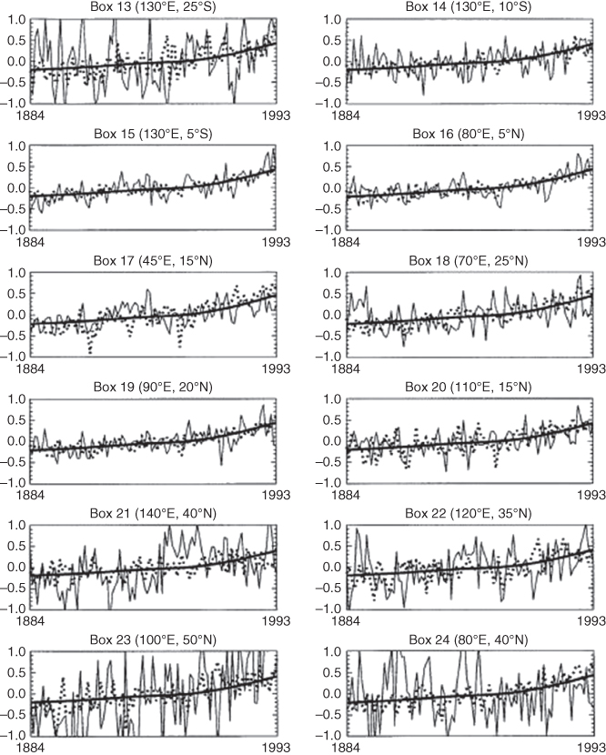
Figure 11.11 Continued from Figure 11.10.
(North and Wu (2001). © American Meteorological Society. Used with permission.)
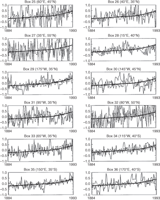
Figure 11.12 Continued from Figure 11.11.
(North and Wu (2001). © American Meteorological Society. Used with permission.)
The signals used in the North and Wu (2001) paper were taken from earlier work in a dissertation by Stevens (1997). We show here a few figures which illustrate the time dependence of the signals. Figure 11.9 shows the global average signal (actually the average over the 36 boxes shown as black squares in Figure 11.8. The topmost panel shows the faint solar signal, the next lower is the stratospheric aerosol signal from volcanic particles left after eruptions. The sharp dips going backward in time are Mt Pinatubo in 1992, then El Chichon, then Mt Agung. The next lower panel shows both the greenhouse gas and tropospheric aerosol signals. Note the anti-collinearity of these two global signals, making it very difficult to discriminate between them in a detection scheme. The lowermost panel shows the time dependence of the sum of all four signals.
Figure 11.13 shows the same 36 stations. In this figure, signals are band-pass filtered in what Stevens called the “solar band,” a frequency band straddling the frequency 1/10 ![]() . The squares of the real and imaginary parts of the Fourier frequency components are shown as columns above the stations. The amplitude is the square root of the sum of these two parts (site by site). Note that both of the imaginary parts are dominant over the real parts. This simply means that the phase lag is nearly
. The squares of the real and imaginary parts of the Fourier frequency components are shown as columns above the stations. The amplitude is the square root of the sum of these two parts (site by site). Note that both of the imaginary parts are dominant over the real parts. This simply means that the phase lag is nearly ![]() , as expected from a gradual temporal increase in the signal. The important thing about this figure is that the two panels show a strong asymmetry between the hemispheres. This asymmetry should assert some discriminating power between the two signals and help us to distinguish one from the other in our detection process.
, as expected from a gradual temporal increase in the signal. The important thing about this figure is that the two panels show a strong asymmetry between the hemispheres. This asymmetry should assert some discriminating power between the two signals and help us to distinguish one from the other in our detection process.

Figure 11.13 The real and imaginary parts squared for the Fourier component of the greenhouse gas forcing (a) and the tropospheric aerosol forcing (b). The Fourier frequency component is at a period of one decade. The imaginary part dominates in both upper and lower panels, suggesting that the phase lag is  . The important point is that there is considerable asymmetry between the two hemispheres, suggesting a good possibility of discriminating between the two signals.
(North and Stevens (1998). © American Meteorological Society. Used with permission.)
11.4.7 Characterizing Natural Variability
When Stevens selected the 36 boxes of Figure 11.8, he tried to space them so that there was as little correlation as possible. If there were no correlation, the 36-dimensional vector with unity in position one and zeroes elsewhere would be the first normalized EOF, and so on. This suggests that only a small rotation of the natural variability field will be necessary to generate the EOFs. It might also mean that the procedure will not be very sensitive to our choice of model-generated fields to use in our study. Nevertheless, North and Wu (2001) decided to use not only the EBM-generated EOFs but also to use several (one 1000 year run from the Max Planck Institute (ECHAM1/LSG), two 1000 year runs from different GFDL models, and one 1000 year run from the Hadley Centre (HadCM2)) GCM-generated sets. We could then compare them to see if there is much difference. Recall that even if we do not use the best set, we do not bias the result, but our estimate might be slightly suboptimal with respect to error variance with our estimators. That comparison will be indicated in the figures to follow in this chapter.
With four signals, it is best to recognize that the problem is equivalent to multiple regression for the signal amplitudes. The filter formalism we have used so far gets more complicated because we must make sure that for each of the four signals, the other three have no component parallel to that which is passed through and optimally weighted. On the basis of standard multiple regression analysis, the optimal estimator for a particular ![]() is given by
is given by
where ![]() . In (11.74), the quantity
. In (11.74), the quantity ![]() is a diagonal matrix with diagonal entries given by the components of the signal vector. The matrix
is a diagonal matrix with diagonal entries given by the components of the signal vector. The matrix ![]() is the inverse space–time lagged covariance matrix of the natural variability in its EOF or diagonal form,
is the inverse space–time lagged covariance matrix of the natural variability in its EOF or diagonal form, ![]() , where
, where ![]() is the covariance matrix. It forms a metric tensor in space (Hasselmann, 1993; also see the Appendix of North and Wu, 2001).
is the covariance matrix. It forms a metric tensor in space (Hasselmann, 1993; also see the Appendix of North and Wu, 2001).
The formalism leads to a similar expression to that of the single-signal case:

The matrix ![]() can be formed as the array of the
can be formed as the array of the ![]() ,
,
Then the covariance matrix of the estimators ![]() and
and ![]() is just
is just
11.4.8 Detection Results
The results of the North and Wu (2001) paper are compactly summarized in chart form in Figure 11.14. This graphic shows the results for a total of five experiments, the asterisk indicating that the estimate is based on 20 tropical stations with 100 year records. The ![]() symbol indicates the 36 stations and 100 years of data as in the previous figure. The
symbol indicates the 36 stations and 100 years of data as in the previous figure. The ![]() symbol indicates that the experiment was for 43 stations—20 with 100 years record and 23 with only 50 years; the
symbol indicates that the experiment was for 43 stations—20 with 100 years record and 23 with only 50 years; the ![]() symbol indicates the experiment was conducted with 72 stations—36 with 50 years record and 36 with 100 years records;
symbol indicates the experiment was conducted with 72 stations—36 with 50 years record and 36 with 100 years records; ![]() is based on 72 stations with 50 years of data (1944–1993). The error bars in the figure represent a 90% confidence region. If an error bar reaches below the dotted line (zero) the corresponding
is based on 72 stations with 50 years of data (1944–1993). The error bars in the figure represent a 90% confidence region. If an error bar reaches below the dotted line (zero) the corresponding ![]() coefficient is not significant at the 90% level. The clusters labeled GFCLc, GFDLml, EBCM, ECHAM1/LSG, and HadCM2 are used to indicate that these experiments were conducted with the EOFs generated from long (usually 1000 years, but 10 000 years for the EBM).
coefficient is not significant at the 90% level. The clusters labeled GFCLc, GFDLml, EBCM, ECHAM1/LSG, and HadCM2 are used to indicate that these experiments were conducted with the EOFs generated from long (usually 1000 years, but 10 000 years for the EBM).

Figure 11.14 Estimates of signals using natural variability from GFDLc, GFDLml, EBM, MPI, and HadCM2, and using the EBM-generated signals for  , and
, and  . This graphic also shows the results for a total of five experiments. The asterisk indicates that the estimate is based on 20 tropical stations with 100 year records. The
  symbol indicates that 36 stations and 100 years of data as in the previous figure. The
  symbol indicates that the experiment was for 43 stations—20 with 100 year records and 23 with only 50 year records; the
  symbol indicates the experiment was conducted with 72 stations—36 with 50 year records and 36 with 100 year records;
  is based on 72 stations with 50 years of data (1944–1993).
(Figure from North and Wu (2001). (©Amer. Meteorol. Soc., with permission).)
We can examine each row individually to sort out the main features. The top row representing the detection of the solar cycle shows quite a few dips below the dotted line, indicating that in many experiments it was not significantly different from zero (i.e., the zero-amplitude hypothesis could not be rejected). As we scan the different natural variability choices, we see there is rather good consistency; further, it is the rightmost experiment with only 50 years of data that is most unstable, which is hardly surprising because temporally, less data have been included (less than five solar cycles). The greenhouse gas (second) row shows very tight error bars and the estimates of the ![]() -signal strength seem very robust across the different experiments and across the different choices of natural variability. The volcanic signal (third row) shows wider error bars but with unanimous statistical significance. There are not that many volcanic events in the record. Finally, the fourth row showing the aerosol signal strength shows many overlaps with the zero line and very unstable results across all possible configurations. Each estimate seems to have very precise error bars, but there is strong dependence on all factors. We would have to conclude that no aerosol signal has been detected.
-signal strength seem very robust across the different experiments and across the different choices of natural variability. The volcanic signal (third row) shows wider error bars but with unanimous statistical significance. There are not that many volcanic events in the record. Finally, the fourth row showing the aerosol signal strength shows many overlaps with the zero line and very unstable results across all possible configurations. Each estimate seems to have very precise error bars, but there is strong dependence on all factors. We would have to conclude that no aerosol signal has been detected.
Next consider the ellipses in Figure 11.15 which represent the different elements of ![]() , the covariance of the estimators for signals
, the covariance of the estimators for signals ![]() and
and ![]() . Look first at the upper left corner. The collinearity of
. Look first at the upper left corner. The collinearity of ![]() and
and ![]() are quite evident across all of the five ellipses in the box. An error on the small side of
are quite evident across all of the five ellipses in the box. An error on the small side of ![]() is correlated with a similar small estimate of
is correlated with a similar small estimate of ![]() . Note that all the ellipses intersect
. Note that all the ellipses intersect ![]() , meaning that it fails the significance test. Other figures in the diagram can be interpreted in a similar way.
, meaning that it fails the significance test. Other figures in the diagram can be interpreted in a similar way.

Figure 11.15 Error ellipses of pairs of signals, given five different model prescriptions for the natural variability: GFDLc (solid line); GFDLml (dotted line); MPI (dashed line); EBM (dashed-dotted line); HadCM2 (dashed-dotted-dotted line). Here (a), (b), and (c) are EBCM signals for 72 stations, 36 with 100 years of data, 36 with 50 years of data; (d)–(f) are EBM signals for 72 global sites all with 50 years of data; (g)–(i) are HadCM2  and
and  and EBM
  and
and  signals for 72 global sites all with 50 years of data.
(Figure from North and Wu (2001). (© Amer. Meteorol. Soc., with permission).)
11.4.8.1 Convergence
In this section, we examine the convergence of the estimation process. Figures 11.16 and 11.17 show the convergence results. The abscissa shows the number of space–time EOF modes included in the partial sum up to that many terms. The EOFs are arranged in order of descending variance (eigenvalue). We can see from (1a), (1b), (1c), and (1d) that all of the series converge. We already know that ![]() and
and ![]() are unstable statistically. Panels (1e) and (4e) show this by the irregularity of the amplitude estimate
are unstable statistically. Panels (1e) and (4e) show this by the irregularity of the amplitude estimate ![]() as a function of EOF number. The estimate of
as a function of EOF number. The estimate of ![]() even drops below zero. On the other hand, the estimates of
even drops below zero. On the other hand, the estimates of ![]() and
and ![]() are quite stable, both converging consistently to a value around 0.60.
are quite stable, both converging consistently to a value around 0.60.

Figure 11.16 (1a)–(1e) For solar cycle (S), (2a)–(2e) for greenhouse gas (G), (3a)–(3e) for volcanic (V), and (4a)–(4e) for aerosol (A) in the case of the 36 global stations over 100 years. The space–time EOF modes are arranged in order of descending variance (EOFs from 10,000 year EBM control run). (1a)–(4a) The normalized cumulative fraction of variance of the signal,  with
with  . (1b)–(4b) indicate the eigenvalue of each spatial–temporal mode; (1c)–(4c) indicate the contributions to
  from the individual EOF modes; (1d)–(4d) indicate the cumulative
  . (1e)–(4e) The cumulative estimate of
  including EOFs up to
  .
.
(Figure from North and Wu (2001). (©Amer. Meteorol. Soc., with permission).)
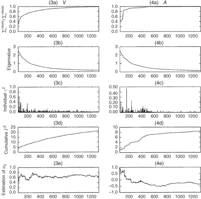
Figure 11.17 Continued from the previous figure.
(Figure from North and Wu (2001). (©Amer. Meteorol. Soc., with permission).)
11.4.9 Discussion of the Detection Results
We suggest two reasons that the North and Wu (2001) study yields a somewhat lower estimate than expected amplitude for ![]() and
and ![]() as well as the near-zero amplitude for
as well as the near-zero amplitude for ![]() . The Appendices of North and Wu (2001) contain a number of interesting tests of the detection program. For example, Figure 11.18 shows results of a Monte Carlo experiment using the EOFs from the 10,000 year run of the EBM for the natural variability (EOFs) and all four signals are included with
. The Appendices of North and Wu (2001) contain a number of interesting tests of the detection program. For example, Figure 11.18 shows results of a Monte Carlo experiment using the EOFs from the 10,000 year run of the EBM for the natural variability (EOFs) and all four signals are included with ![]() . Then 200 of the EBM 50 year runs are used as “data” inserted into the 72 data sites. In the figure, the error ellipses for 90% confidence are drawn along with the individual points representing each run. Note that each ellipse has (1, 1) at its center. In the left panel, the correlation of
. Then 200 of the EBM 50 year runs are used as “data” inserted into the 72 data sites. In the figure, the error ellipses for 90% confidence are drawn along with the individual points representing each run. Note that each ellipse has (1, 1) at its center. In the left panel, the correlation of ![]() and
and ![]() is evident. In the right panel the orthogonality is expressed as virtually no correlation between the errors in
is evident. In the right panel the orthogonality is expressed as virtually no correlation between the errors in ![]() and
and ![]() .
.
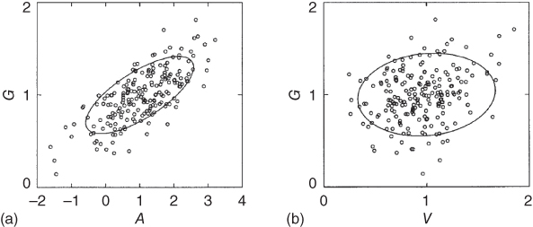
Figure 11.18 (left) Scatter plot of Monte Carlo studies and 90% error ellipse of detection studies for the pair of signal G–A for 72 boxes all with 50-yr (1944–93) observational data. In Monte Carlo studies, the artificial data is constructed by adding 200 50-yr EBCM control run and four EBCM signals S, G, V, and A. The truncated eigenmode is 500 in the 10 k yr control run of EBCM. (right) Same as (a) except for pair of signal G–V.
(Figure from North and Wu (2001). (©Amer. Meteorol. Soc., with permission).)
Another interesting test is shown in Figure 11.19. Here, the comparison of the time dependence of ![]() with that of
with that of ![]() (
(![]() and
and ![]() are omitted in the experiment), where the solid line is the EBM signal, the light solid line indicates the GCM HadCM2, and the dotted line represents the GCM ECHAM4. The EBM signal is very close to those of the two GCMs. One can notice a very slight difference between the two signals (panels (a) and (b)) with the aerosols making a slight bend in the
are omitted in the experiment), where the solid line is the EBM signal, the light solid line indicates the GCM HadCM2, and the dotted line represents the GCM ECHAM4. The EBM signal is very close to those of the two GCMs. One can notice a very slight difference between the two signals (panels (a) and (b)) with the aerosols making a slight bend in the ![]() curve. The statistical collinearity is evident in the global average curves. The only difference that can be used for discrimination between them must be in the inter-hemispheric difference (presumably there is higher
curve. The statistical collinearity is evident in the global average curves. The only difference that can be used for discrimination between them must be in the inter-hemispheric difference (presumably there is higher ![]() in the NH. Most GCM simulations have indicated a larger value of
in the NH. Most GCM simulations have indicated a larger value of ![]() that cancels part of a larger
that cancels part of a larger ![]() . This latter would mean that the data point would lie in the upper right end of the ellipses in Figure 11.15a,d. In this case, the “equilibrium sensitivity” would be greater than the nominal 2.3 K that we assume for the EBM used in this book. We cannot rule out this case as it would lie within the 90% confidence area of those two panels of Figure 11.15.
. This latter would mean that the data point would lie in the upper right end of the ellipses in Figure 11.15a,d. In this case, the “equilibrium sensitivity” would be greater than the nominal 2.3 K that we assume for the EBM used in this book. We cannot rule out this case as it would lie within the 90% confidence area of those two panels of Figure 11.15.
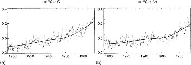
Figure 11.19 (a) First principal component time series of annual mean climate change signal for greenhouse-gas-only forcing from EBCM (heavy solid line), HadCM2 GCM (light solid line), and ECHAM4 GCM (dotted line); (b) same as (a) except for greenhouse-gas-plus-aerosol forcing.
(Figure from North and Wu (2001). (©Amer. Meteorol. Soc., with permission).)
Another possible reason for the discrepancy between the EBM detection study and that of many IPCC GCMs is that the EBM uses only a mixed-layer ocean in its EBM-generated signal. Compared to a deeper ocean coupling, this would make the EBM signal larger than the one which might have been generated from a coupled ocean–atmosphere GCM. The latter would hold down the signal from such a coupled model as we discussed in Chapter 10.
A final possible criticism of the North and Wu (2001) study lies in the fact that so many EOFs are used. Using very large numbers of EOFs often raises a red flag in statistical studies because their eigenvalues are necessarily close together and this means that they will “mix” (if the eigenvalues were close together, a linear combination of the associated eigenvectors is also an eigenvector). But this criticism is false. The (sample) PC time series associated with a particular EOF are orthogonal by construction and the EOFs form a good basis set.
Notes for Further Reading
Surface temperature data sets can be found at the following websites. In many cases, there are descriptions of how the data are processed and how the estimation procedure works:
- 1. The NASA/Goddard Institute for Space Studies (GISS) provides a very accessible digital as well as graphical (including maps) surface temperature data. http://data.giss.nasa.gov/gistemp/.
- 2. The Climate Research Unit (CRU) of the University of East Anglia provides both digital and colorful graphical information. They also provide a list of publications by Dr. Philip D. Jones and his colleagues. http://www.cru.uea.ac.uk/cru/data/temperature/.
- 3. The NOAA/National Climate Data Center (NCDC) website is a little more difficult to navigate, but it has the data. http://www.ncdc.noaa.gov/temp-and-precip/global-maps/.
- 4. NOAA also publishes online the pdfs of annual issues of the Bulletin of the American Meteorological Society on the State of the Climate for each year starting in 1991; there is also a decadal review covering 1981–1990. http://www.ncdc.noaa.gov/bams/past-reports.
Exercises
- 11.1
- a. Consider two measurements of surface temperature at a location. They are described as

where
 is the true temperature and
  and
and  are measurement errors. Assume that measurements are unbiased, that is,
  , and error variance is given by
  and
and  . Further assume that the errors in the two measurements are uncorrelated, that is,
  . Show that an unbiased optimal estimator with the least MSE is given by
- b. Show that an unbiased optimal estimator for three independent unbiased measurements is given by

- c. For
 independent unbiased measurements, the optimal unbiased estimator is obtained by minimizing the so-called error functional defined by

where
 is called a Lagrange multiplier. Show that the optimal unbiased estimator is given by
- d. Show that the error variance of the optimal estimator is given by

- a. Consider two measurements of surface temperature at a location. They are described as
- 11.2 Consider two measurements,
 , of which the errors are correlated. Assume that error covariance matrix is given by

- a. Find the principal axes for which two new measurements are uncorrelated.
- b. Show that the two measurements rotated according to the eigenvectors become uncorrelated.
- c. Determine the optimal unbiased estimator for
 based on the two measurements
  .
.
- 11.3 As discussed in Exercise 11.2, two or more measurements on the surface of the Earth are typically correlated. Let us consider
 measurements of length
  of a variable
  (say, temperature),
  . Then, the covariance matrix of the
  measurements is given by

The eigenvalues and eigenfunctions of are determined by solving the Karhunen–Loève equation

where
 is the
  th eigenvector with corresponding eigenvalue
  . Then, the
  measurements can be written as a unique linear combination of eigenvectors as
This procedure is called the EOF analysis. The unique amplitude time series,
 , is often called the it principal component time series; for this reason, this decomposition is also called the PCA (principal component analysis). The eigenfunctions are orthogonal to each other and eigenvalues are all positive, as the covariance matrix is real and symmetric. In addition, the eigenvectors (also called EOF loading vectors) and PC time series should satisfy the following:

where
 is a proportionality constant.
- a. Show that the covariance matrix,
 , can be written as

- b. Show that the EOF decomposition indeed satisfies the Karhunen–Loève equation and the proportionality constant
 .
. - c. Show how you can calculate the PC time series from the eigenfunctions of the covariance matrix.
- a. Show that the covariance matrix,
- 11.4 Global average temperature is defined by

where
 denotes the surface of the Earth, and
  and
and  represent longitude and latitude of a location
  on the surface of the Earth. The factor
  is introduced to properly scale the result.
- a. Let us consider the problem of estimating global average temperature based on a small number of samples on the surface of the Earth. Set up an optimal estimation problem based on samples
 .
. - b. Solve the optimal estimation problem for the weights.
- a. Let us consider the problem of estimating global average temperature based on a small number of samples on the surface of the Earth. Set up an optimal estimation problem based on samples
- 11.5 Consider a noise-forced one-dimensional energy balance model of the form

- a. Calculate the spectrum of
 using the spectrum of noise forcing
  .
. - b. What is the nature of the spectrum of
 when the model is forced by a white-noise forcing, that is,
  , regardless of the frequency
  ? Plot the spectrum for ocean and land responses by using
  ,
,  W m
W m C)
C) ,
,  =10 years,
  .
. - c. Express the variance of the temperature response in terms of the spectrum of temperature and in terms of the spectrum of forcing.
- d. Calculate the autocovariance function for the temperature response when the model is driven by a white-noise forcing. Then, determine the e-folding timescale of response.
- a. Calculate the spectrum of
- 11.6 Consider a signal detection problem, where the normalized signal at two stations is given in the form

where
 are orthogonal unit vectors. Actual data at the two stations are given by
where
 is the true strength of the signal and
 are the natural variability at the two stations. Thus, the signal of constant strength is embedded amid randomly varying natural variability. Further, assume that
that is, natural variability at each station has mean zero and the random variability at the two stations are uncorrelated.
- a. One way to determine the signal strength is to project the normalized signal on the data set, that is,
 . Show that this is an unbiased estimator of the signal strength. What is the error variance of the signal strength
  ?
? - b. Note that the estimator in Part (a) is not optimal, as it did not consider that the magnitude of natural variability differs at the two stations. One way to account for this is to estimate the signal strength at each station and weigh the two estimates optimally. Develop an optimal estimator based on this idea. Calculate the error variance and compare it with that in Part (a).
- c. Show for the signal and mutually uncorrelated noise background (natural variability) at
 stations that

- where the signal is determined by

- a. One way to determine the signal strength is to project the normalized signal on the data set, that is,
- 11.7 Consider data consisting of four different temporally varying signals on top of natural variability:

where
 denote different signals,
  represents natural variability, and
  space–time points. Assume that the signals are not necessarily orthogonal to each other.
- a. Show that this problem can be recast in terms of EOFs of natural variability in the form

- where
 represents the EOF mode number.
 - b. Show that an unbiased estimator for the signal strength can be derived from each EOF mode equation in Part (a) as

- a. Show that this problem can be recast in terms of EOFs of natural variability in the form