3 Energy Harvesting Thermoelectric and Microsystems Perspectives and Opportunities and Opportunities

Most industrial and transportation processes worldwide waste 50%–70% of the fuel energy input, leading to vast amounts of wasted thermal energy that is both available and recoverable. Recent studies indicate that approximately 12.5 quads of thermal energy are available across a spectrum of transportation platforms, including light-duty vehicles (e.g., passenger vehicles, minivans, and sport utility vehicles), and heavy vehicles (e.g., class 4–class 8 trucks) in the United States alone. Recent additional studies indicate that there are another approximately 10 quads of thermal energy available across a variety of industrial processes, including aluminum, glass, steel, cement, paper and pulp, and other processes in the United States. This energy typically is dissipated to the environment in exhaust and coolant systems of these vehicles and industrial processing plants. Thermoelectric power generation (TEG) is one important technology that is available to recover this energy and convert it to useful electrical energy. TEG systems are typically quiet, low maintenance, capable of high reliability and stealthy operation when designed properly, and can transition gracefully to different power levels when necessary. TEG power technology has been used to recover waste energies in certain niche energy recovery applications (e.g., truck exhausts, wood-burning stoves) and in small combustion-driven systems (e.g., natural gas line sensors). Recent advancements in thermoelectric (TE) materials have created the potential to harness this energy and convert it at much better energy conversion efficiencies (near or greater than 10%) than in past applications. Thermoelectric energy recovery systems using new TE materials have thermal, structural, and thermoelectric design challenges to overcome in designing high-performance, robust, and flexible systems that take advantage of these new materials. Thermoelectric, thermal, and structural considerations are necessarily interdependent in these system designs and must be dealt with simultaneously to satisfy the TE system’s operational requirements and achieve the high performance and robustness desired. This chapter discusses these design challenges and various design and analysis techniques used to overcome them in current and future systems.

Nomenclature

Images

3.2 Thermoelectric Design—Optimization and Constraints

TABLE 3.1 Available Waste Energy Temperatures in Different Economic Sectors

Images

Thermoelectric (TE) technology can recover and convert a portion of the waste heat from a variety of industrial, commercial, transportation, and military systems through temperature differentials between the various exhaust streams or hot environments and cooling environments available in these applications. Table 3.1 shows some typical waste exhaust stream temperatures available in various industrial and transportation applications. The US Department of Energy, Office of Energy Efficiency and Renewable Energy, has performed extensive analysis of petroleum-derived fuel use across the United States [1]. This analysis typically uses separate fuel-use categories for light-duty vehicles, minivans and sport-utility vehicles (SUVs), and medium-/ heavy-duty vehicles. The transportation energy data [1] show that in 2002, for example, the fuel usage by light-duty vehicles, minivans, and SUVs represented approximately 16.27 quads of energy (1 quad = 10¹⁵ Btu). Approximately 35% of this energy was dissipated in the high-temperature exhaust streams of these vehicles; therefore, approximately 5.7 quads of waste thermal energy were available to recover in exhaust streams in this vehicle category in 2002. This same transportation energy data [1] show that in 2002 the fuel usage by medium-/ heavy-duty vehicles was approximately 5.03 quads of energy. Approximately 30% of this energy was dissipated in the high-temperature exhaust streams of these vehicles, so another approximately 1.5 quads of waste thermal energy were available to recover in exhaust streams in this vehicle category in 2002. In 2008, the energy usage in the light-duty vehicle, minivan, and SUV sectors rose to approximately 16.4 quads and the medium-/heavy-duty vehicle sector stayed roughly the same at approximately 5.02 quads [1]. Therefore, the high-temperature waste thermal energy available in these two vehicle sectors has stayed roughly equivalent during that time period.

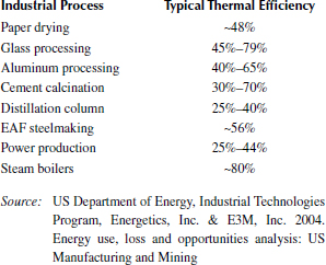
The US Department of Energy Industrial Technologies Program office also has estimated waste thermal energy dissipated in various industrial processes throughout the United States [2,3]. This analysis categorized and characterized waste thermal energy in industrial processes such as aluminum smelting, glass processing, steel processing, paper and pulp processing, cement processing, and several others. The analysis found considerable waste of thermal energy in these industrial processes and, therefore, highly significant opportunities for industrial waste heat recovery. Table 3.2 shows typical process efficiencies for some of these processes [2].

Tables 3.1 and 3.2 show that there are enormous amounts of industrial waste thermal energy available for recovery and that waste occurs at temperatures that are quite compatible with the temperature-dependent performance of many TE materials discussed in other chapters in this handbook. Estimates indicate there are approximately 10 quads of waste thermal energy available in various industrial processes and about 1.8 quads of this waste thermal energy are recoverable [2], meaning it is at temperatures where it could be recovered.

TABLE 3.2 Typical Process Efficiencies in Key us Industrial Processes and Applications

Images

Waste heat in these exhaust streams and processes can be recovered either within a heat exchanger integrated with a TE device hot side tied directly into the exhaust stream (i.e., real-time recovery) or by storing it in a thermal energy storage medium for use in the future. New opportunities for efficiently recovering waste heat have been created because of advances in micro-and nanotechnologies. The key to identifying TE waste heat recovery applications is to determine when thermal exchange between existing process fluids in a given system is not an available option or provides no useful technical or economic benefit, or when electrical power generated by TE systems has a beneficial intrinsic value within the system.

Extensive system-level research has been performed in the past 5 years to design TE systems to recover and convert waste thermal energy to useful electrical energy in various industrial and transportation systems. This work has been useful in demonstrating what TE conversion efficiencies and power levels are possible with newer, advanced TE materials (i.e., skutterudites, lead–antimony–silver–telluride nanocomposites, half-Heuslers) and more conventional TE materials (i.e., bismuth telluride) in these different waste energy applications.

Designing TE generator systems for these waste heat recovery (WHR) applications typically involves two processes: design optimization, which follows design techniques discussed in Angrist [7] and Rowe [8], and design performance prediction, which follows techniques discussed in Hogan and Shih [9], Hendricks et al. [10], and Crane [11].

3.2.1 TE Design Optimization

Design optimization generally involves maximizing the TE conversion efficiency, TE power output, power density, specific power (i.e., power per mass), or other relevant design parameter for the TE system or application of interest. The TE conversion efficiency, η, is typically given by

η = P / Q h (3.1)

$η = P / Q_{h} (3.1)$

where P = power output and Q_h is the thermal energy input to the TE hot side [7,8]. The power output is generally given by

P = [( N \cdot α \cdot Δ T ) 2 ( N \cdot R i n t + R o ) 2 \cdot R o] (3.2)

$P = [\frac{(N \cdot α \cdot Δ T)^{2}}{(N \cdot R_{i n t} + R_{o})^{2}} \cdot R_{o}] (3.2)$

where

R_int and R_o are familiar internal and external load resistances, respectively

ΔT = T_h – T_c

T_h = TE device hot-side temperature

T_c = TE device cold-side temperature

α = |α_p| + |α_n| for a single couple

This equation indicates the multiplier, N, the number of couples in a device, for a multiple couple system.

Optimization of conversion efficiency for a given set of TE materials and TE element geometries is discussed at length in Angrist [7] and Rowe [8] and leads to the well-known relationship:

η max = (P Q h) max = ⎡ ⎣ T h - T c T h ⎤ ⎦ \cdot ⎡ ⎣ ( 1 + Z * T ¯ ¯ ¯ ) 1 / 2 - 1 ( 1 + Z * T ¯ ¯ ¯ ) 1 , 2 + T c T h ⎤ ⎦ (3.3)

$η_{\max} = (\frac{P}{Q_{h}})_{\max} = [\frac{T_{h} - T_{c}}{T_{h}}] \cdot [\frac{(1 + Z^{*} \bar{T})^{1 / 2} - 1}{(1 + Z^{*} \bar{T})^{1, 2} + \frac{T_{c}}{T_{h}}}] (3.3)$

where T¯¯¯=(Th+Tc)/2 $\bar{T} = (T_{h} + T_{c}) / 2$ . Recent design optimization techniques have leveraged these basic equations to develop more sophisticated analysis and optimization algorithms because, in most waste heat recovery and TE power system designs, the external exhaust and ambient temperatures, T_exh and T_amb, are usually known more clearly as requirements or bounding conditions. Consequently, it is difficult to surmise a priori what the best combination of T_h and T_c for a given TE material set will be in any given waste heat recovery application, or whether maximum efficiency conditions, maximum power, or maximum power density conditions are going to be the most appropriate system parameters to optimize. In addition, and more importantly, it is necessary to couple the TE device optimization closely with the hot-side and cold-side thermal design optimization to create high-performance TE power systems. This necessarily requires one to analyze and optimize the TE design based on the external exhaust and ambient temperatures, T_exh and T_amb, in any given application.

Hendricks and Lustbader [4,5] first began investigating this and developing more powerful optimization techniques that laid the foundation for the advanced optimization techniques discussed later. Their approach created a “system of optimization design equations” that coupled the hot-side heat transfer, Q_h, and cold-side heat transfer, Q_c, design optimization with the TE device design optimization. The analysis considers the TE system schematically represented in Figure 3.1 where a simple, multiple-couple TE system is depicted. This type of system configuration is common whether one is considering bulk elements or thin-film elements.

Images

Figure 3.1 Industrial or vehicle thermoelectric energy recovery system schematic.

Angrist [7] and Rowe [8] discuss that the amount of heat required on the TE device hot side, Q_h, is given by

Q h = N \cdot [α \cdot I \cdot T h - 1 2 \cdot I 2 \cdot (p p γ p + p n γ n + 2 \cdot R c o n t a c t, h) + (κ p \cdot γ p + κ n \cdot γ n) \cdot (T h - T c)] (3.4a)

$Q_{h} = N \cdot [α \cdot I \cdot T_{h} - \frac{1}{2} \cdot I^{2} \cdot (\frac{p_{p}}{γ_{p}} + \frac{p_{n}}{γ_{n}} + 2 \cdot R_{c o n t a c t, h}) + (κ_{p} \cdot γ_{p} + κ_{n} \cdot γ_{n}) \cdot (T_{h} - T_{c})] (3.4a)$

From Equations (3.2) and (3.4a) it can be deduced with straightforward mathematics that the amount of cold-side heat dissipated, Q_c, is given by

Q c = N \cdot [α \cdot I \cdot T c + 1 2 \cdot I 2 \cdot (p p γ p + p n γ n + 2 \cdot R c o n t a c t, c) + (κ p \cdot γ p + κ n \cdot γ n) \cdot (T h - T c)] (3.4b)

$Q_{c} = N \cdot [α \cdot I \cdot T_{c} + \frac{1}{2} \cdot I^{2} \cdot (\frac{p_{p}}{γ_{p}} + \frac{p_{n}}{γ_{n}} + 2 \cdot R_{c o n t a c t, c}) + (κ_{p} \cdot γ_{p} + κ_{n} \cdot γ_{n}) \cdot (T_{h} - T_{c})] (3.4b)$

The current, I, and resistance, R_int, are given by

I = N \cdot α \cdot ( T h - T c ) N \cdot R i n t + R o (3.5)

$I = \frac{N \cdot α \cdot (T_{h} - T_{c})}{N \cdot R_{i n t} + R_{o}} (3.5)$

R i n t = P P ¯ ¯ ¯ ¯ ¯ + p n ¯ ¯ ¯ ¯ + R c o n t a c t (3.6)

$R_{i n t} =^{\underline{P_{P}}} +^{\underline{p_{n}}} + R_{c o n t a c t} (3.6)$

and

α = | α p | + | α n | and R c o n t a c t = R c o n t a c t, h + R c o n t a c t, c .

$α = | α_{p} | + | α_{n} | and R_{c o n t a c t} = R_{c o n t a c t, h} + R_{c o n t a c t, c} .$

The voltage of the system is given by

V o = I \cdot R o = α \cdot Δ T - I \cdot R i n t (3.7)

$V_{o} = I \cdot R_{o} = α \cdot Δ T - I \cdot R_{i n t} (3.7)$

on a per-couple basis. Angrist [7], Cobble [12], and Rowe [8] show that this entire system of equations (Equations (3.2) and (3.4–3.7)) can be optimized to achieve the maximum conversion efficiency, η_max, when

γ n γ p = p n κ p p p κ n - - - - - \sqrt (3.8)

$\frac{γ_{n}}{γ_{p}} = \sqrt{\frac{p_{n} κ_{p}}{p_{p} κ_{n}}} (3.8)$

This is basically a TE element design requirement, and Z^* in Equation (3.2) is given by

Z * = α 2 [ p n κ n - - - - \sqrt + p p κ p - - - - \sqrt ] 2 (3.9)

$Z^{*} = \frac{α^{2}}{[\sqrt{p_{n} κ_{n}} + \sqrt{p_{p} κ_{p}}]^{2}} (3.9)$

Furthermore, the maximum efficiency with respect to external resistance is achieved when

m o p t = (R o N \cdot R i n t) o p t = (1 + 6) 2 + (1 + 6) Z * T ¯ ¯ ¯ - - - - - - - - - - - - - - - \sqrt (3.10)

$m_{o p t} = (\frac{R_{o}}{N \cdot R_{i n t}})_{o p t} = \sqrt{(1 + 6)^{2} + (1 + 6) Z^{*} \bar{T}} (3.10)$

where δ = (R_contact/R_int).

Hendricks and Lustbader [4,5] formulated this set of optimization equations into a set of self-consistent design optimization equations given by

[Q h N \cdot γ n] o p t = f q (T h, T c) (3.11a)

$[\frac{Q_{h}}{N \cdot γ_{n}}]_{o p t} = f_{q} (T_{h}, T_{c}) (3.11a)$

(I γ n) o p t = f i (T h, T c) (3.11b)

$(\frac{I}{γ_{n}})_{o p t} = f_{i} (T_{h}, T_{c}) (3.11b)$

(V N) o p t = f v (T h, T c) (3.11c)

$(\frac{V}{N})_{o p t} = f_{v} (T_{h}, T_{c}) (3.11c)$

(γ n γ p) o p t = p n κ p p p κ n - - - - - \sqrt = f g (T h, T c) (3.11d)

$(\frac{γ_{n}}{γ_{p}})_{o p t} = \sqrt{\frac{p_{n} κ_{p}}{p_{p} κ_{n}}} = f_{g} (T_{h}, T_{c}) (3.11d)$

η max = (P Q h) max = ⎡ ⎣ T h - T c T h ⎤ ⎦ \cdot ⎡ ⎣ m o p t - 1 - 6 m o p t + ( 1 + 6 ) T c T h ⎤ ⎦ = f η (T h, T c) (3.11e)

$η_{\max} = (\frac{P}{Q_{h}})_{\max} = [\frac{T_{h} - T_{c}}{T_{h}}] \cdot [\frac{m_{o p t} - 1 - 6}{m_{o p t} + (1 + 6) \frac{T_{c}}{T_{h}}}] = f_{η} (T_{h}, T_{c}) (3.11e)$

These are functions of only temperatures T_h and T_c because the TE material properties generally are functions of temperature in any design optimization or design performance analysis. Recognizing the importance of hot-side and cold-side heat transfer and heat exchanger performance in heat recovery systems, Hendricks and Lustbader completed the system optimization analysis for TE systems depicted in Figure 3.1 by simultaneously including the design analysis for the hot-side and cold-side heat exchangers. Their analysis includes hot-side and cold-side heat losses by parametrically accounting for them with heat loss factors, β_hx, β_h,TE, β_cx, and β_c,TE, which are basically heat loss fractions of incoming energy to a given heat exchanger or interface. The thermal equation for the heat transfer supplied by the hot-side heat exchanger to the TE device then becomes

Q h, T E = ( T e x h - T h . ) \cdot ( 1 - β h , T E ) [ 1 m ˙ h \cdot C p , h \cdot ε h ( 1 - β h x ) + R t h , h ] (3.12)

$Q_{h, T E} = \frac{(T_{e x h} - T_{h} .) \cdot (1 - β_{h, T E})}{[\frac{1}{{\dot{m}}_{h} \cdot C_{p, h} \cdot ε_{h} (1 - β_{h x})} + R_{t h, h}]} (3.12)$

The thermal equation for the heat transfer dissipated by the cold-side heat exchanger from the TE device then becomes

Q c, T E = ( T c - T a m b ) [ ( 1 . - β c x . ) m ˙ c C p , c ε c + R t h , c ] \cdot ( 1 - β c , T E ) (3.13)

$Q_{c, T E} = \frac{(T_{c} - T_{a m b})}{[\frac{(1 . - β_{c x} .)}{{\dot{m}}_{c} C_{p, c} ε_{c}} + R_{t h, c}] \cdot (1 - β_{c, T E})} (3.13)$

The heat loss fractions are generally defined as the amount of heat loss compared to the heat loss entering a given component, whether it be within the heat exchangers themselves or the interfaces at which heat is entering or leaving the TE device hot side or cold side. Therefore, the heat loss fractions are generally defined as

β h, T E = Q 1 o s s , h , T E Q h , T E β hx = Q 1 o s s , h , e x Q h , e x β c, T E = Q 1 o s s , c , T E Q c , T E β c x = Q 1 o s s , c , e x Q c , e x

$\begin{matrix} β_{h, T E} = \frac{Q_{1 o s s, h, T E}}{Q_{h, T E}} & β_{hx} = \frac{Q_{1 o s s, h, e x}}{Q_{h, e x}} & β_{c, T E} = \frac{Q_{1 o s s, c, T E}}{Q_{c, T E}} & β_{c x} = \frac{Q_{1 o s s, c, e x}}{Q_{c, e x}} \end{matrix}$

R_th,h and R_th,c in Equations (3.12) and (3.13) are the sum of all thermal resistances at the interface between the TE device and the hot-side and cold-side heat exchangers, respectively. Energy balance requirements then couple these thermal transfer relationships to the TE design optimization equations in Equations (3.11a)–(3.11e) to complete the system design optimization. Figure 3.1 shows that this was basically a four-lumped-node design optimization model that simultaneously accounted for heat exchanger and TE device performance in the design optimization. This set of optimization equations specified the family of optimum TE designs, including the number of couples, p-type and n-type element areas, voltage and current output, power and maximum conversion efficiency for any given T_h and T_c, and a specific exhaust temperature, T_exh, and ambient temperature, T_amb.

This design optimization analysis is required in waste energy recovery applications because what is usually known are the exhaust flow conditions and ambient temperatures in a given waste energy recovery environment or situation. The goal is to identify the best T_h and T_c conditions at which to operate to create the maximum conversion efficiency or power output, important information about the TE design at those conditions, and performance sensitivities and trade-offs around these optimum design points. The optimum selection of T_h and T_c involves critical trade-offs in conversion efficiency, power, and hot-side and cold-side thermal transport in any given waste energy recovery application. These trade-offs are demonstrated in Figure 3.2 and the associated discussion. In fact, this is the case in most TE power generation analyses and applications whether they are necessarily waste energy recovery related or not.

Images

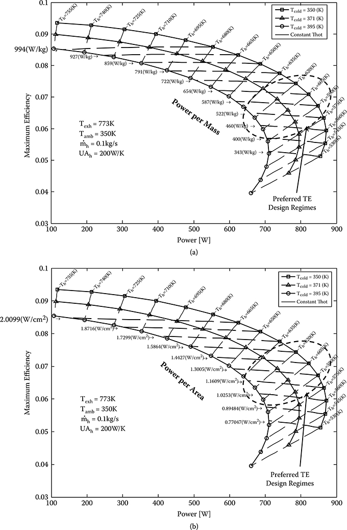
Figure 3.2 Maximum efficiency–power output map for typical TAGS: PbTe [21,22] TE element designs: UA_h = 200 W/ K, T_exh = 773 K, T_amb = 350 K.

Figure 3.2 shows typical results produced from this optimization analysis in the form of maps depicting the relationship between maximum efficiency and power (maximum efficiency–power) that can be created for any TE energy recovery system design and any set of temperature-dependent TE material properties. Two different maximum efficiency–power maps are shown: (a) one with constant specific power lines superimposed, and (b) one with constant power-per-area lines superimposed on the map. These analyses were performed using typical p-type TAGS-85 and n-type PbTe thermoelectric properties [21,22], but they can be created for any p-type/ n-type TE material combination, including segmented element designs. These maps are quite powerful in the amount of information that is conveyed in one design optimization map. They are generally created for a given exhaust temperature, ambient temperature, hot-side heat exchanger UA_h (defined in Section 3.3), and exhaust mass flow rate, m˙h ${\dot{m}}_{h}$ .

The main efficiency–power curves represent the loci of optimum designs having maximum efficiency and the plotted power at varying TE hot-side temperatures, T_h, and cold-side temperatures, T_c. The shape of these curves is produced directly from the coupling and interaction between the hot-side heat exchanger performance (and heat transfer) and the TE device performance in the optimization analysis described by Equations (3.11)–(3.13). As T_h increases for a given T_c, the TE device efficiency increases, but for a constant T_exh and UA_h the hot-side heat transfer is decreasing. Consequently, the power increases with the TE efficiency up to a point where maximum power is achieved, after which the power decreases because hot-side heat transfer decreases too much to offset the TE efficiency increase. Each optimum design along these curves has a different number of couples, N; optimum p-type and n-type element area, A_p and A_n; and current, I, as T_h and T_c combinations vary as shown in Figure 3.2. These curves first clearly demonstrate the trade-off between maximum efficiency and power for the conditions of a given exhaust stream, T_exh, UA_h, and m˙h ${\dot{m}}_{h}$ in typical waste energy recovery applications. The constant hot-side temperature lines help to identify where TE designs with equivalent T_h lie and their relationship to one another in efficiency and power. The efficiency–power curves tend upward and to the right (efficiency and power increasing) as either or both T_exh and UA_h increase in magnitude. The analytical power of these curves is that they effectively and rapidly provide the opportunity to identify and investigate multiple TE system designs throughout the potential design domain for a given waste heat recovery application.

Figure 3.2(a) also shows lines of constant specific power (power per TE device mass). The mass accounted for here is only estimates of the TE device mass, including insulating ceramics, copper interconnections straps, and the TE elements themselves. It is clear in Figure 3.2(a) that specific power generally increases as one transitions into regions of higher maximum efficiency. Figure 3.2(b) also shows lines of constant power flux (power per area), which also can be related to the hot-side heat flux because of the maximum efficiency information included in the map. It is clear that power flux increases as one moves into regions of higher maximum efficiency, which can have significant ramifications in applications where TE device miniaturization is critical.

These maximum efficiency–power maps show the potential points of optimum design and the efficiency–power sensitivities and design trade-offs available for given waste heat recovery applications. These maps can be generated for any selection of p-type and n-type TE materials discussed in other chapters of this book, and for any particular single-material element or segmented-element design. They also define “preferred TE design regimes” or preferred optimum design regions, which are superior because of (1) their higher maximum efficiency with only a small power penalty, and (2) their higher specific power performance.

Hendricks and Lustbader [4,5] also extended the design optimization techniques described earlier and, based on Equations (3.11a)–(3.11e), to segmented-element optimization using the techniques described in Swanson, Somers, and Heikes [13]. The same types of maximum efficiency–power maps discussed before can be generated in the resulting segmented-element design optimization analyses.

Additional numerical, system-level, TE design optimization has been demonstrated by Crane [14], Crane and Bell [15,16], and Crane and Jackson [17]. Constrained, nonlinear minimization functions were defined to solve the multi-parameter design problems using either gradient-based, genetic algorithms or a hybrid of the two approaches. A better understanding of the interactions between various design variables and parameters can be gained from this type of multiparameter optimization approach. More than 20 different design variables, including fin and TE dimensions and dozens of different design parameters, can be optimized. A selection of different design constraints includes minimum power density, maximum hot-and cold-side pressure drops, maximum total mass, and minimum output power. Additional constraints include maximum TE surface temperatures and maximum temperature gradients across the TE elements to help improve design robustness. Choices for analysis objective function include maximum gross or net power, maximum efficiency, and maximum gross or net power density, which can be based on either total mass or TE mass. An optimization analysis can be conducted once the design variables, parameters, constraints, and objective function have been selected. The result is a nominal design that can be fine-tuned through parametric analysis on selected variables and parameters and then used in an operating model where the design conditions can vary.

3.2.2 TE Design Performance

TE system design performance is the second stage of the design process where an optimum design identified in the design optimization process is then analyzed for a variety of nominal and off-nominal design conditions. A more sophisticated multiple-node and/ or multiple-volume analysis is typically employed at this stage. Analytically exact techniques have been described by Sherman, Heikes, and Ure [18] for p–n TE couple designs shown in Figure 3.1. Hogan and Shih [9] describe a typical performance analysis approach based on solving Domenicali’s equation [19] for one-dimensional energy balance in the p-type and n-type elements within a device:

\partial \partial x (κ (x) \cdot \partial T ( x ) \partial x) = - p \cdot J 2 + J \cdot T (x) \cdot \partial α ( x ) \partial x (3.14)

$\frac{\partial}{\partial x} (κ (x) \cdot \frac{\partial T (x)}{\partial x}) = - p \cdot J^{2} + J \cdot T (x) \cdot \frac{\partial α (x)}{\partial x} (3.14)$

and the equation for heat flux within the elements:

q (x) = J \cdot T (x) \cdot α (x) - κ (x) \cdot \partial T ( x ) \partial x (3.15)

$q (x) = J \cdot T (x) \cdot α (x) - κ (x) \cdot \frac{\partial T (x)}{\partial x} (3.15)$

These equations are valid in typical parallelepiped or constant diameter cylindrical TE elements used in most typical TE devices. Mahan [20] and Hogan and Shih [9] describe how Equations (3.14) and (3.15) can be reformulated into a coupled set of first-order differential equations for T(x) and q(x) within the TE element design given by

κ (x) \cdot d T ( x ) d x = J \cdot T (x) \cdot α (x) - q (x) (3.16)

$κ (x) \cdot \frac{d T (x)}{d x} = J \cdot T (x) \cdot α (x) - q (x) (3.16)$

d q ( x ) d x = p (x) \cdot J 2 \cdot [1 + Z (x) \cdot T (x)] - J \cdot α ( x ) \cdot q ( x ) κ ( x ) (3.17)

$\frac{d q (x)}{d x} = p (x) \cdot J^{2} \cdot [1 + Z (x) \cdot T (x)] - \frac{J \cdot α (x) \cdot q (x)}{κ (x)} (3.17)$

Hogan and Shih [9] originally presented Equation (3.17) as

d q ( x ) d x = p (x) \cdot J 2 \cdot [1 - Z (x) \cdot T (x)] - J \cdot α ( x ) \cdot q ( x ) κ ( x )

$\frac{d q (x)}{d x} = p (x) \cdot J^{2} \cdot [1 - Z (x) \cdot T (x)] - \frac{J \cdot α (x) \cdot q (x)}{κ (x)}$

This has since been shown to be a typographical error in reference 9, per discussions with Hogan (July 19, 2010) and an errata sheet that shows the correction as shown in Equation (3.17).

Hogan and Shih discuss how coupled Equations (3.16) and (3.17) can be solved for T(x) and q(x) profiles in the TE element with iterative numerical analysis techniques and appropriate boundary conditions on the cold-side and hot-side temperatures of given a TE device. The p-type and n-type elements are typically nodalized into a number of finite isothermal TE layers in the lengthwise direction (i.e., x-direction) as shown in Figure 3.3. Equations (3.16) and (3.17) are applied in a finite-difference formulation at each ith layer to yield

T i + 1 = T i + Δ x K i \cdot (I \cdot T i \cdot α i - q i) (3.18)

$T_{i + 1} = T_{i} + \frac{Δ x}{K_{i}} \cdot (I \cdot T_{i} \cdot α_{i} - q_{i}) (3.18)$

q i + 1 = q i + [p i \cdot J 2 \cdot (1 + α 2 i . \cdot T i p i κ i) - J \cdot α i \cdot q i K i] \cdot Δ x (3.19)

$q_{i + 1} = q_{i} + [p_{i} \cdot J^{2} \cdot (1 + \frac{α_{i}^{2} . \cdot T_{i}}{p_{i} κ_{i}}) - \frac{J \cdot α_{i} \cdot q_{i}}{K_{i}}] \cdot Δ x (3.19)$

Images

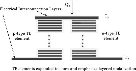
Figure 3.3 Typical isothermal layer nodalization used in TE elements in iterative numerical techniques in solving Equations (3.16) and (3.17).

This formulation corrects the typographical error in reference 9 per discussions with Hogan (July 19, 2010) and an errata sheet created. This technique does not necessarily couple the q(x) profile with hot-side and cold-side heat exchanger performance, but it does provide useful T(x) and q(x) information for any given T_h and T_c conditions of interest and provides required hot-side heat transfer, Q_h, and cold-side heat transfer, Q_c, that the heat exchangers must accommodate.

In order to truly perform a system-level design performance analysis, the solution to these differential equations must be coupled with hot-side and cold-side heat exchanger analysis. Hendricks et al. [10] have recently used thermoelectric analysis routines within the ANSYS^® version 12.0 analysis software package, which solve relationships similar to Domenicali’s equation (Equation (3.14)) within a TE device design subject to appropriate thermal boundary conditions, to perform this type of system-level design performance analysis. This type of analysis relies on characterizing the UA_h of the hot-side heat exchanger design using a given hot-side exhaust temperature and mass flow rate entering the heat exchanger design and details of the heat exchanger structure and interfaces. The ANSYS^® version 12.0 software analysis code generally allows one also to nodalize the TE elements as shown in Figure 3.3; it uses variational principles and finite volume techniques applied to the conservation of energy and continuity of electric charge to solve a set of simultaneous equations for heat flow, current, and temperatures within the TE elements under transient or steady-state conditions [23]. Under steady-state conditions, these relationships in their most general, three-dimensional form are given by

\nabla \cdot (T \cdot [α] \cdot J \to) - \nabla \cdot ([κ] \cdot \nabla \to T) = q ˙ (3.20)

$\nabla \cdot (T \cdot [α] \cdot \vec{J}) - \nabla \cdot ([κ] \cdot \vec{\nabla} T) = \dot{q} (3.20)$

\nabla \cdot ([0] \cdot [α] \cdot \nabla \to T) - \nabla \cdot ([0] \cdot E \to) = 0 (3.21)

$\nabla \cdot ([0] \cdot [α] \cdot \vec{\nabla} T) - \nabla \cdot ([0] \cdot \vec{E}) = 0 (3.21)$

where

[α] = Seebeck coefficient matrix

[σ] = electrical conductivity matrix

[κ] = thermal conductivity matrix

J→ $\vec{J}$ = current density vector

E→ $\vec{E}$ = electric field intensity vector

T = temperature

The heat generation term, q˙ $\dot{q}$ , in Equation (3.20) generally contains the ρ · J² heat dissipation term in Domenicali’s equation. These general relationships converge down to Domenicali’s relationships in one-dimensional analyses depicted in Figure 3.3. The power of the ANSYS^® analysis is that it allows any temperature-dependent thermoelectric properties to be used in each of the nodalized layers in Figure 3.3, so that it is straightforward to model segmented element designs in a system design. Furthermore, ANSYS^® 12.0 theoretically allows one to couple the solution of Equations (3.20) and (3.21) to hot-side and cold-side heat exchanger performance models to produce system-level predictions.

Images

Figure 3.4 Typical TE module efficiency-power maps for varying external resistance and current.

The results of such an analysis produce TE module efficiency–power maps similar to those shown in Figure 3.4. These maps show the module efficiency–power for various external load resistances and temperature differentials that are created across the TE module directly because of the interaction and coupling of the TE device and hot-side and cold-side heat exchanger performance. The external resistance ratios (R_o/ N·R_int) and temperature differentials ΔT = (T_h –T_c) are superimposed on the module efficiency–power curves in Figure 3.4. The analysis includes the effect of interface contact resistance and parasitic thermal losses. It is clear in the Figure 3.4 results how temperature differential, ΔT = (T_h –T_c), increases across the TE module as the external load resistance increases. This is the direct result of the trade-off between system voltage and current and TE heat flows, power, and conversion efficiency as the external resistance is varied.

The analysis in Figure 3.4 was performed for exhaust flow temperature, T_exh, from 780 to 733 K, exhaust mass flow rate, m˙h ${\dot{m}}_{h}$ of 0.16 kg/s, and a UA_h of approximately 377 W/K; however, the analysis can be performed at various exhaust flow conditions, T_exh, exhaust mass flow rate, m˙h ${\dot{m}}_{h}$ , and heat exchanger performance characterized by the UA_h. Figure 3.4 also shows, for example, a typical impact of reducing the exhaust temperature, T_exh, from 795 to 748 K alone on the power output and module efficiency. The benefit of depicting the analysis results in this manner is that the maximum efficiency and maximum power points, and their relationship to one another and other nonoptimum performance points, in the overall potential operating performance space can be quickly and clearly seen. Critical design performance decisions concerning various operating points then can be made quickly and intelligently with regard to what the entire design performance envelope looks like.

One noteworthy and clearly identified performance characteristic is that the point of maximum power occurs at an external resistance condition of R_o > N · R_int in this type of design performance analysis, because it is performed at constant T_exh and T_amb conditions and not constant T_h and T_c conditions. In fact, Figure 3.4 demonstrates clearly that ΔT does not stay constant along the module efficiency–power curves. Hendricks et al. [10] discuss the reasons for this, which are directly tied to the TE power output relationship in Equation (3.2). Determining the external resistance that defines maximum power point when ?T is not constant leads to the following relationship described in Hendricks et al. [10]:

R o, o p t = N \cdot R i n t + 2 \cdot R o , o p t \cdot ( N \cdot R i n t + R o , o p t ) Δ T \partial (Δ T) \partial R o (3.22)

$R_{o, o p t} = N \cdot R_{i n t} + \frac{2 \cdot R_{o, o p t} \cdot (N \cdot R_{i n t} + R_{o, o p t})}{Δ T} \partial (Δ T) \partial R_{o} (3.22)$

This relationship clearly shows that the optimum external resistance that maximizes power is greater than N·R_int. In fact, this equation can ultimately be cast into a quadratic relationship for R_o,opt, which can be explicitly solved for R_o,opt in any given design performance analysis.

Figure 3.4 also clearly shows that the maximum TE module efficiency condition occurs at R_o,opt value where

(R o , o p t N \cdot R i n t) e f f i c i e n c y > (R o , o p t N \cdot R i n t) p o w e r > 1 (3.23)

$(\frac{R_{o, o p t}}{N \cdot R_{i n t}})_{e f f i c i e n c y} > (\frac{R_{o, o p t}}{N \cdot R_{i n t}})_{p o w e r} > 1 (3.23)$

which are both greater than 1. However, the maximum module efficiency–power point can be quite close in magnitude to the maximum power condition. Therefore, in waste heat recovery applications and other TE power generation applications where ΔT is not constant, one must not assume that the [R_o,opt/(N·R_int)] = 1 condition applies. Each particular design performance analysis must establish these operating points and their relationship to one another in any given waste heat recovery application.

3.2.3 Sectioned TE Design Optimization

Table 3.1 shows that there are many waste heat recovery applications where available exhaust gases and exhaust streams could be at high temperatures and, therefore, provide large temperature differentials across TE waste heat recovery devices. This is especially true if effective thermal cooling techniques can keep cold-side temperatures low. Large available temperature differentials create the opportunity to utilize a relatively advanced TE design technique called “sectioned design.” With high exhaust stream temperatures and therefore large temperature differentials, the exhaust flow through the hot-side heat exchangers in a TE waste heat recovery system can undergo relatively large temperature drops along the flow length as it transfers its thermal energy to the TE device hot side. In addition, the hot-side thermal transfer decreases significantly along the flow length. Consequently, the TE devices within the design can experience large differences in hot-side temperature and hot-side thermal transfer as the exhaust flow temperature decreases. It is impossible to design one optimal TE device that operates at maximum performance levels as hot-side temperature and thermal flows significantly decrease in these situations. One would therefore like to create optimum TE device designs that accommodate this change in hot-side temperature and hot-side thermal transfer as they decrease with flow length. Sectioned design allows this type of TE device optimizing as the exhaust flow conditions change with flow length. Figure 3.5 schematically shows a typical example of this type of “dual-sectioned TE design” approach where the exhaust flow temperatures decrease significantly along the flow length, and the TE hot-side temperatures in each of the two sections are quite different.

Images

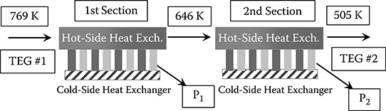
Figure 3.5 Typical dual-sectioned TE system design.

Any number of sections can be added to satisfy given design requirements in any waste heat recovery application, but the actual measurable performance benefits gained are dependent on the magnitude of the overall (T_exh – T_amb) temperature differential available. Cost considerations and system complexity issues often constrain the maximum number of sections to about three. This was the number of sections described by Crane, LaGrandeur, and Bell [6]. Each TE section was optimized for a particular temperature and heat flux range in the direction of gas flow. This helps avoid TE incompatibility in the direction of fluid flow [15]. The TE section nearest the hot gas inlet comprised TE couples made of two-stage segmented elements to account for the large temperature gradient and heat flux between the hot and cold heat exchangers. Located axially downstream of the high-temperature TE section in the direction of gas flow, the medium-temperature TE section also is made up of two-stage segmented elements of the same materials as the high-temperature TE section. However, these elements are thinner than the elements in the high-temperature TE section due to the lower heat flux and temperature gradient. Segmented elements are not required for the lowest temperature TE section. Each of these TE sections can be operated on one electrical current or on different electrical circuits, allowing for more optimal current densities per TE section.

The design optimization and design performance analysis techniques discussed can generally be used to design each of the sections. However, there are unique and complex design trade-offs associated with the amount of heat transferred, the conversion efficiency, and power generated in each section. These must be fully evaluated in any TE energy recovery system design to achieve the optimum performance. Figure 3.6 illustrates some of these trade-offs in a simple dual-sectioned design shown in Figure 3.5. The dual-sectioned design creates significant design trade-offs between power output and efficiency in each section when seeking the optimum overall system performance, whether that is maximum overall system efficiency or maximum system power output. There are two sets of maximum efficiency–power curves in Figure 3.6; one for section 1 designs using lead–antimony–silver–telluride (LAST) materials and a second for section 2 designs using bismuth telluride materials in Figure 3.5. The maximum efficiency–power curves identify the loci of maximum efficiency designs defined by techniques in Equations (3.11)–(3.13). The resulting maximum efficiency–power maps in each section are produced by the coupled interdependence of the TE device design and hot-side and cold-side heat exchangers in sections 1 and 2.

Figure 3.6 illustrates a tremendous amount of design optimization information for the two sections of this dual-sectioned design. The section 1 efficiency–power curves show the various maximum efficiency–power points for several different hot-side and cold-side temperature combinations (T_h,1, T_c,1) resulting from the coupled interaction between the TE device design and hot-side heat exchanger design characterized by a UA_h = 375 W/ K. These curves show the range and domain of efficiency and power combinations possible in section 1, with inevitably different TE couples and p-type and n-type TE areas at each design point on the curve. The design analysis does identify the TE couples and TE areas required at each design point, although this information is not explicitly shown on the curves. The hot-side heat exchanger design and its performance at each T_h,1 along the section 1 efficiency–power curves then produce unique entrance exhaust temperatures to section 2 (shown in Figure 3.5). This situation creates a family of maximum efficiency–power curves for the section 2 design, one for each of the section 1 T_h,1 conditions along the section 1 curves. Figure 3.6 shows four such section 2 design curves corresponding to four selected design points on the section 1 curve for a cold-side temperature condition of 312 K.

Images

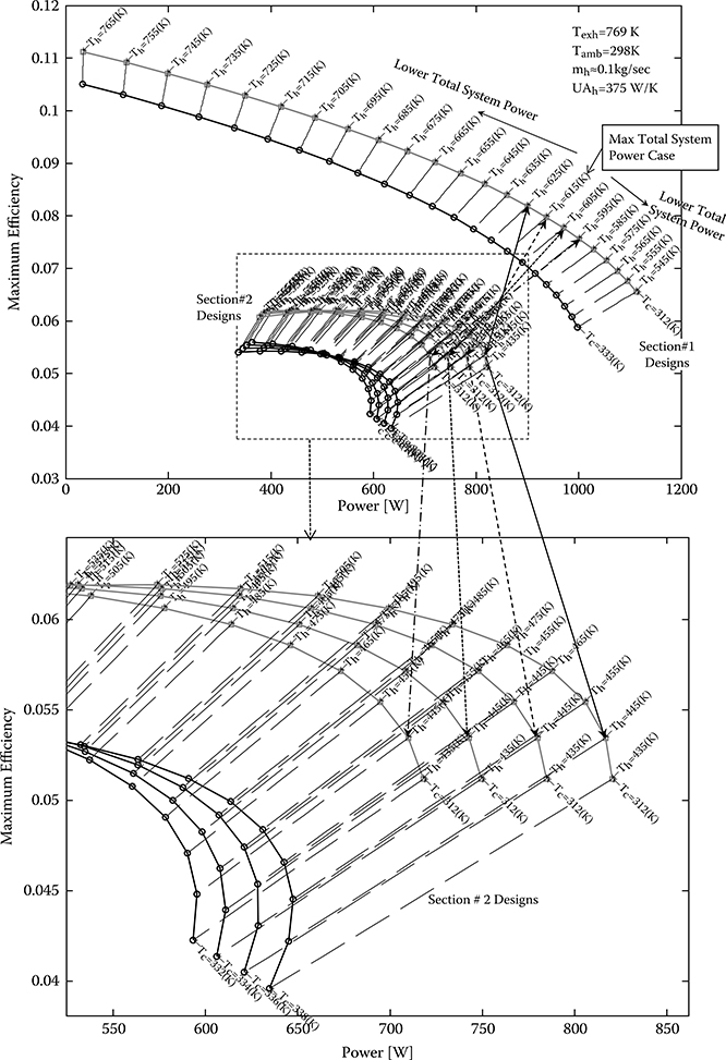
Figure 3.6 Typical dual-sectioned analysis results for T_exh = 769 K, m˙h ${\dot{m}}_{h}$ = 0.1 kg/s, UA_h = 375 W/ K, T_amb = 298 K.

As the section 1 design changes, efficiency and power output varies and, therefore, impacts input exhaust temperature on section 2. There is a uniquely defined section 2 maximum efficiency–power curve that dictates its efficiency–power characteristics resulting from the coupled performance of the TE device designs and the hot-side heat exchanger design in section 2. The four section 1 points selected for T_c,1 = 312 K demonstrate that, as section 1 power decreases and efficiency increases, the section 2 power output generally increases while the section 2 efficiency stays roughly the same. This section 2 efficiency is largely governed by the TE material properties for bismuth telluride materials at the temperatures used in section 2. Different section 2 TE materials and properties would exhibit different efficiency–power sensitivities and performance.

This behavior and interactions between sections 1 and 2 create a maximum total system power point because the increases in section 2 power only offset or override the section 1 decreases in power up to a point. The maximum total system power point generally does not occur even close to the maximum point for section 1. Understanding this design power trade-off and knowing where the maximum total system power point resides are critical to designing a dual-sectioned system to satisfy any given efficiency–power requirement, whether maximum efficiency or maximum power is of paramount interest in a given energy recovery application. This behavior and interaction between section 1 and section 2 designs can occur in general at any common cold-side temperature (T_c,1 and T_c,2) conditions, as shown in Figure 3.6, and in general for any combination of TE materials in the two sections. Figure 3.6 also shows the maximum efficiency–power reduction that occurs as cold-side temperatures increase (black lines for sections 1 and 2). In both of these cases, the maximum total power point may shift as a result of the impact of TE material performance or cold-side temperature effects on power output and it is crucial to quantify this shift if it occurs. These design interactions become more complex as more sections are added in a multiple-sectioned design.

3.2.4 Transient Design Performance

Steady-state models discussed earlier give an effective means to choose a nominal design point and optimize the design for a particular set of operating conditions. However, a thermoelectric generator in waste heat recovery applications may see a variety of operating conditions, which change frequently as a function of time. A primary example of this application is exhaust heat recovery in an automobile or heavy truck. In this case, a TEG is integrated into a car or truck exhaust stream and the exhaust temperature and mass flow conditions result from the transient engine load conditions dictated by the particular drive cycle that the vehicle experiences. Figure 3.7 shows an example of the temperatures and mass flows downstream of the catalytic converter in the exhaust system that are produced in a new European drive cycle (NEDC), a common automotive drive cycle used in European countries.

In order to model the TEG in different drive cycles and other dynamic operating conditions, steady-state models for TE couples and devices are defined first. Energy balance equations are described by Crane [11] as follows with locations shown schematically in Figure 3.8:

Images

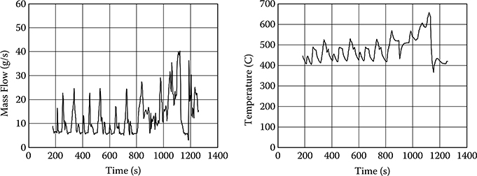
Figure 3.7 Time-dependent exhaust gas mass flow and temperature downstream of the catalytic converter for an inline 6 cylinder, 3.0 L displacement engine operating on the new European drive cycle (NEDC).

Images

Figure 3.8 Schematic of TE subassembly with heat exchangers (HEXs) showing model temperature locations.

Q h 1 + 1 2 I 2 R c o n n, h - U A T E - c o n n (T c e n, h - T h 1) = 0 (3.24)

$Q_{h 1} + \frac{1}{2} I^{2} R_{c o n n, h} - U A_{T E - c o n n} (T_{c e n, h} - T_{h 1}) = 0 (3.24)$

Q h 2 + 1 2 I 2 R c o n n, h - U A T E - c o n n (T c e n, h - T h 2) = 0 (3.25)

$Q_{h 2} + \frac{1}{2} I^{2} R_{c o n n, h} - U A_{T E - c o n n} (T_{c e n, h} - T_{h 2}) = 0 (3.25)$

U A T E - c o n n (T c e n, h - T h 1) + U A T E - c o n n (T c e n, h - T h 2) - U A c r o s s, c o n n (T s h 2 - T c e n, h) = 0 (3.26)

$U A_{T E - c o n n} (T_{c e n, h} - T_{h 1}) + U A_{T E - c o n n} (T_{c e n, h} - T_{h 2}) - U A_{c r o s s, c o n n} (T_{s h 2} - T_{c e n, h}) = 0 (3.26)$

h A h (T s h 2) - U A c r o s s, c o n n (T s h 2 - T c e n, h) - h A n a t (T s h 2 - T \infty) + U A c r o s s, c h, h, 1 - 2 (Δ T s h 1) - U A c r o s s, c h, h, 2 - 3 (Δ T s h 2) = 0 (3.27)

$\begin{matrix} h A_{h} (T_{s h 2}) - U A_{c r o s s, c o n n} (T_{s h 2} - T_{c e n, h}) - h A_{n a t} (T_{s h 2} - T_{\infty}) \\ + U A_{c r o s s, c h, h, 1 - 2} (Δ T_{s h 1}) - U A_{c r o s s, c h, h, 2 - 3} (Δ T_{s h 2}) = 0 \end{matrix} (3.27)$

m C p h h Δ T f h - h A h (T f h - T s h 2) = 0 (3.28)

$m {}_{h}C_{p h} Δ T_{f h} - h A_{h} (T_{f h} - T_{s h 2}) = 0 (3.28)$

where

Q h, i = α \cdot I \cdot T h, i + K \cdot Δ T T E - 1 2 \cdot I 2 \cdot (R T E + 2 R c o n t a c t) (3.29)

$Q_{h, i} = α \cdot I \cdot T_{h, i} + K \cdot Δ T_{T E} - \frac{1}{2} \cdot I^{2} \cdot (R_{T E} + 2 R_{c o n t a c t}) (3.29)$

Equations (3.24) and (3.25) represent conductive heat transfer from the TE elements into their connectors. Equations (3.26) and (3.27) represent conductive heat transfer from these connectors through the fluid-carrying channel wall by way of the fins to fluid convective heat transfer connectors. They include the losses due to natural convection and radiation (Equation 3.29). is an energy balance equation for convective heat transfer into the fluid. is the standard equation for thermoelectric heat flow in power generation. The model solves these governing equations simultaneously for steady-state temperatures at each node in the direction of flow. The number of simultaneous equations varies with the number of TE elements in the direction of fluid flow.

These energy balance equations were then translated into differential equations based on Equation (3.30) and integrated into the S-function template of MATLAB^®/ Simulink^®:

m v o l C p d T d t = Q 1 - Q 2 (3.30)

$m_{v o l} C_{p} \frac{d T}{d t} = Q_{1} - Q_{2} (3.30)$

The (m_vol C_p) term in Equation (3.30) represents the thermal mass of each control volume. This could be a TE element, TE connector, heat exchanger, or fluid thermal mass depending on the control volume. The direction of heat flow is important to make sure that the signs for Q₁ and Q₂ are correct. Otherwise, the differential equations cannot be solved correctly.

A baseline for the transient model is the optimized design from the steady-state model. Inputs for the model are similar to those of the steady-state model. Operating condition inputs include the hot-and cold-side inlet temperatures and flows and external electrical load resistance. External electrical load resistance can be set equal to the internal resistance of the TEG or it can be set at a particular constant external load. A simulated electrical load controller can be attached to the model as an additional Simulink block in order to model the effects of a varying electrical load that is not necessarily optimal. Outputs for the model are again similar to those of the steady-state model.

The model can be operated in a stand-alone mode as is or the S-function can be cut and pasted into a larger systems-level model. BMW and Ford have both used versions of this model in their larger automotive systems-level models [6]. The model can be run using single hot-side inlet flow and temperature conditions or using the hot-side inlet flow and temperature conditions for a drive cycle.

Images

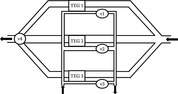
Figure 3.9 Schematic of multiple parallel section TEG (V stands for valve).

Additional systems-level attributes have been added to the transient model to aid in its use as part of a larger system. A maximum hot inlet temperature can be defined to prevent TE element overheating or overheating of any other part of the TEG device. A maximum hot flow can be defined to prevent excessive backpressure in the system, which can reduce engine performance if the TEG is integrated into the exhaust system of a vehicle. In addition, to better match the thermal impedance of a dynamic thermal system as defined in Crane and Bell [16], the TEG can be broken into a number of TE sections in parallel (see Figure 3.9) as opposed to sections in a series as described earlier. Having multiple TE sections can allow the TEG to operate better at low flows when the design has been optimized for higher flow rates as each of the parallel sections can be operated together or in various advantageous combinations.

Figure 3.10, a transient simulation example, shows the time-dependent power output, hot-side fluid, and TE surface temperatures for the TEG being driven toward steady-state by a set of constant operating conditions from an initial set of conditions. The temperature curves in these figures are at different axial positions on the TEG in the direction of flow as a function of time. The colder the temperatures are, the farther they are from the TEG inlet. Figure 3.11, another transient simulation example, shows efficiency and power output along with the TE surface and hot-side fluid temperatures for the TEG for an NEDC automotive drive cycle. The importance of these analysis results is that they quantify and highlight the response time of this system design in this energy recovery application. This is an important design metric that is impacted by a specific system’s component weights and volumes as well as the materials and fluids used throughout the system design. System transient response is also governed by other design parameters, such as the exhaust temperature and mass flow rate and ambient environmental conditions, and it requires knowledge of the specific heats and density of each material and fluid used throughout the design. It must be characterized for each specific design and for each specific set of operating conditions, boundary conditions, and environments anticipated or of interest in a given energy recovery application. The amount of work required to produce credible and accurate transient response analyses should not be underestimated.

Images

Figure 3.10 Simulated outputs for the transient TEG model using constant operating conditions. Temperature graphs show temperatures as a function of time at different axial positions along the TEG in the direction of fluid flow. The hottest temperature curves are nearest to the TEG hot gas inlet, while the coldest are nearest to the TEG hot gas outlet.

3.3 Thermal System Design and Considerations in Thermoelectric Systems

3.3.1 Thermal System Design Relationships

Many waste energy recovery applications in today’s environment require solutions that are compact, environmentally friendly, quiet, vibration free, without ozone-impacting fluids, and highly reliable with few or no moving parts. Advanced thermo-electric energy recovery and conversion systems envisioned in the future for waste energy recovery applications generally require that a temperature differential be maintained across the TE device while the required thermal energy is transferred in/ out of the system. In any event, nearly isothermal interfaces are required on the hot and cold sides of the TE device to achieve predictable maximum performance conditions. Therefore, heat exchanger configurations that transfer the thermal energy in or out of the device must be capable of providing these nearly isothermal conditions on the interfaces with the TE conversion device and operating under their influence. Furthermore, these heat exchangers will have significant weight and volume requirements on their design to assist in minimizing overall heat recovery system weight and volume.

Images

Figure 3.11 Simulated outputs for the NEDC automotive drive cycle using an optimized TEG from the steady-state model. Temperature graphs show temperatures as a function of time at different axial positions along the TEG in the direction of fluid flow. The hottest temperature curves are nearest to the TEG hot gas inlet, while the coldest are nearest to the TEG hot gas outlet.

One must realize the importance of heat transfer at both the hot side and cold side of any TE energy recovery system. A simple rewrite of Equation (3.1) (and Equation (3.3) for maximum efficiency conditions) demonstrates the relationship between TE device efficiency and these hot-side and cold-side (and parasitic loss) thermal transfers:

η = P Q h = Q h - Q 1 o s s - Q c Q h . (3.31)

$η = \frac{P}{Q_{h}} = \frac{Q_{h} - Q_{1 o s s} - Q_{c}}{Q_{h}} . (3.31)$

This simple relationship focuses on the thermal transfers involved in creating the power from the TE system.

Hendricks [25–27] describes the use of the ε–NTU (number of transfer units) analysis method [20] for various basic heat exchanger configurations, counterflow, parallel flow, cross flow, and parallel counterflow. It is clear from Kays and London [24] that heat exchanger effectiveness, ε, is generally expressed by the following relationship for any flow configuration:

ε = ε [NTU, (C min C max /), flow configuration] . (3.32)

$ε = ε [NTU, (\frac{C_{\min}}{C_{\max}}), flow configuration] . (3.32)$

The ε relationship in Equation (3.32) is generally a rather complex one for the various heat exchanger flow configurations. In a heat exchanger that is providing or creating a nearly isothermal interface on one side as it transfers thermal energy, the ratio

[C min C max /] \to 0 (3.33)

$[\frac{C_{\min}}{C_{\max}}] \to 0 (3.33)$

and the Equation (3.32) relationship generally simplifies to

ε = 1 - exp [- U A C min] . (3.34)

$ε = 1 - \exp [\frac{- U A}{C_{\min}}] . (3.34)$

In the advanced waste energy recovery and conversion systems considered herein, it is highly desirable that any heat exchangers coupled with the advanced TE energy conversion system should satisfy the nearly isothermal interface condition and should therefore closely follow the ε relationship in Equation (3.34). Heat exchanger design techniques and “TE design sectioning” techniques are usually employed to help ensure this condition as closely as possible. UA, the overall heat transfer conductance times the heat transfer surface area, and C_min are defined by Kays and London [24]. The UA_h or UA_c of typical hot-side or cold-side heat exchanger designs is evaluated by the techniques shown in Kays and London [24] and typically given by

U A h = (1 \sum i R t h , h , i) o r U A c = (1 \sum i R t h , c , i) (3.35)

$\begin{matrix} U A_{h} = (^{\frac{1}{\sum_{i} R_{t h, h, i}}}) & o r & U A_{c} = (^{\frac{1}{\sum_{i} R_{t h, c, i}}}) \end{matrix} (3.35)$

where the thermal resistances R_th,h,i and R_th,c,I account for all the convective thermal resistance effects of the flow and all the conductive thermal resistance effects of the heat exchanger structures. Evaluation of the thermal resistances R_th,h,i and R_th,c,I is therefore specific to any given hot-side and cold-side heat exchanger designs and the application. The quantity C_min is given by Cmin=m˙h⋅Cp,h $C_{\min} = {\dot{m}}_{h} \cdot C_{p, h}$ or Cmin=m˙c⋅Cp,c $C_{\min} = {\dot{m}}_{c} \cdot C_{p, c}$ , depending on whether one is considering the hot-side heat exchanger or the cold-side heat exchanger, respectively.

UA_h and UA_c (Equation 3.35) are used in Equations (3.12) and (3.13) to determine the hot-side and cold-side heat transfers on the TE devices. In general, UA_h and UA_c are dependent entirely on the heat exchange fluids used, flow conditions, and the structure of the heat exchanger in any given WHR application. There can be a wide variety of heat exchanger structures and they can demonstrate some rather unique and innovative concepts. Figure 3.12 shows an example of a particularly simple and common design known as a flat-plate, parallel-extended-fin design that will be used for illustrative purposes only. The UA of this type of structure is dependent on the heat transfer coefficient in the flow channels and the thermal conductance of the structure itself. The UA of this simple structure is given by

Images

Figure 3.12 Common flat-plate, parallel-extended-fin heat exchanger structure.

U A = 1 [ 1 η F \cdot h c \cdot A f + Δ t κ s t \cdot W \cdot L ], (3.36)

$U A = \frac{1}{[\frac{1}{η_{F} \cdot h_{c} \cdot A_{f}} + \frac{Δ t}{κ_{s t} \cdot W \cdot L}]}, (3.36)$

where h_c = channel heat transfer coefficient, η_F = fin thermal transfer efficiency, A_f = total fin and base heat transfer area, and κ_st = thermal conductivity of the plate structure (and usually the fins themselves).

The thermal conductance term in Equation (3.36) is generally straightforward to evaluate and quantify as is the fin efficiency and fin area. However, the heat transfer coefficient, h_c, is generally a function of channel Reynolds number, Re, and the Prandtl number, Pr, of the fluid [28]. There are a number of different heat transfer correlations of the following form:

h c \propto K 1 1 D h \cdot Re m \cdot P r n (3.37)

$h_{c} \propto \frac{K_{11}}{D_{h}} \cdot {Re}^{m} \cdot P r^{n} (3.37)$

where D_h = channel hydraulic diameter, κ_fl = fluid thermal conductivity, and m ~ 0.5–0.8 and n ~ 0.33. Therefore, the heat transfer coefficient, h_c, is dependent on the fluid properties and the channel velocities and, therefore, the mass flow rate through the heat exchanger, as well as the channel dimensions, w_ch and H. The Reynolds number is generally given by

Re = γ 1 1 \cdot V c h \cdot D h μ 1 1

$Re = \frac{γ_{11} \cdot V_{c h} \cdot D_{h}}{μ_{11}}$

where V_ch = fluid channel velocity, γ_fl = fluid density, and μ_fl = fluid viscosity.

In addition, the heat transfer coefficient is not constant throughout the flow length, generally starting out high at the flow entrance and decreasing with flow length. This is another important motivation for sectioned TE designs discussed in Section 3.2 because the actual heat transfer into the TE device hot side can decrease with flow length. Therefore, one generally desires to have slightly different TE device design along the flow length to truly optimize system performance as the UA_h decreases with flow length. Consequently, even this simple flow arrangement has some subtle and sometimes difficult challenges in evaluating the heat exchanger UA. There are many other heat exchanger configurations that are much more complex than this; the evaluation of their UA values is much more complex and often requires detailed thermal models. It is not possible to discuss how to evaluate the UA of every possible heat exchanger design option in this work. Suffice it to say that it is imperative to analyze the specific convective heat transfer conditions and environments and the conductive heat transfer of the heat exchanger structure properly when evaluating various heat exchanger design options in any given TE WHR system design.

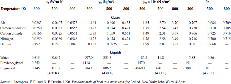
In waste heat recovery applications, the heat exchanger fluids used vary from different gases (i.e., air, nitrogen, helium) to different liquids (i.e., water, water–glycol mixtures, oil). Many of these gases are major constituents of typical waste heat exhaust flows. The fluids’ properties can vary significantly and are critical to the UA evaluation and heat exchanger performance as discussed earlier. Generally, the UA of heat exchangers using gases is low due to their generally low thermal conductivity, low Pr, and Equation (3.37) relationships, which make the first term in the denominator of Equation (3.36) dominate the UA evaluation. The UA of heat exchangers using liquids can be quite high because of their high thermal conductivity and high Pr; therefore, the first term in the denominator of Equation (3.36) becomes quite low. Table 3.3 shows the typical values for common heat exchanger fluids in WHR applications and provides a good comparison between typical gas and liquid properties. These properties and the resulting heat exchanger UA are critical factors in determining what fluids to select in WHR applications because these directly determine the temperature differential, ΔT = T_h – T_c, across the TE device and therefore the TE device performance. Hendricks [26,27] presents the representative UA values of some heat exchanger designs with different fluids, but the UA evaluation is generally quite application specific using the relationships discussed previously. It is not possible to quote specific UA values for all the different and innovative gas and liquid heat exchanger options and configurations in WHR applications, but for a given heat exchanger volume, the UA of liquid heat exchangers is generally an order of magnitude or more higher than the UA of gas heat exchangers.

In detailed system modeling, whereby the heat exchanger can be broken up or nodalized lengthwise with sufficient refinement, the UA can get small enough that effectiveness in Equation (3.33) can be approximated with

ε = 1 - exp [- U A C m ln] \approx U A C m ln = U A h m ˙ h \cdot C p , h o r U A c m ˙ c \cdot C p , c (3.38)

$ε = 1 - \exp [\frac{- U A}{C_{m \ln}}] \approx \frac{U A}{C_{m \ln}} = \frac{U A_{h}}{{\dot{m}}_{h} \cdot C_{p, h}} o r \frac{U A_{c}}{{\dot{m}}_{c} \cdot C_{p, c}} (3.38)$

TABLE 3.3 Typical Fluid Properties of Common Gases and Liquids

Images

Equations (3.12) and (3.13) then reduce to

Q h, T E = ( T e x h - T h ) \cdot ( 1 - β h , T E ) [ 1 U A h \cdot ( 1 - β h x ) + R t h , h ] (3.39)

$Q_{h, T E} = \frac{(T_{e x h} - T_{h}) \cdot (1 - β_{h, T E})}{[\frac{1}{U A_{h} \cdot (1 - β_{h x})} + R_{t h, h}]} (3.39)$

Q c, T E = ( T c - T a m b . ) [ ( 1 - β c x ) U A c + R t h , c ] ( 1 - β c , T E ) (3.40)

$Q_{c, T E} = \frac{(T_{c} - T_{a m b} .)}{[\frac{(1 - β_{c x})}{U A_{c}} + R_{t h, c}] (1 - β_{c, T E})} (3.40)$

It is also quite important to evaluate the pressure drops associated with convective heat exchangers as one endeavors to increase the UA by modification of heat exchanger channel dimensions and overall geometry. The pressure drop through the heat exchanger is generally given by relationships of the form

Δ P e x \propto f (Re) \cdot γ 11 \cdot V 2 c h (3.41)

$Δ P_{e x} \propto f (Re) \cdot γ_{11} \cdot V_{c h}^{2} (3.41)$

where f(Re) is the friction factor. There is a close relationship between the heat exchanger UA and its pressure drop. As channel dimensions decrease, the heat transfer coefficient increases through Equation (3.37) because the flow channel velocities generally increase for a given mass flow rate and the hydraulic diameter decreases. However, the pressure drop and, therefore, pumping power also increase as the channel dimensions decrease. It has been shown that there are actually optimum values of UA as a function of heat exchanger pressure drop [26,27]. This UA–pressure drop optimization is application specific and must be quantified along with optimizing TE device performance to maximize overall TE system performance in any given WHR application. It is crucial that these optimization processes be performed in an integrated and strongly coupled manner in the overall TE system design. This is why analyses in Figures 3.2 and 3.6 are so critical in the TE system design optimization.

3.3.2 Microtechnology Heat Exchangers in TE Systems

In the energy recovery applications found in the transportation sector and industrial processing sector, there is generally a large amount of waste energy available to be captured and converted. This can range from 10s of kilowatts to megawatts of available thermal energy. There is also a general requirement to develop compact, lightweight, and low-cost energy conversion and heat exchange systems in any WHR design application. Therefore, in almost all applications the heat exchange systems must satisfy a general requirement to transfer very high heat fluxes (i.e., 10–100 W/ cm²) across nearly isothermal interface conditions. This is particularly true of the unique energy conversion systems using advanced TE conversion materials envisioned in the next 5–10 years.

Microchannel heat exchangers are one heat transfer technology that is capable of providing this high performance. Their high performance is due to their small channel sizes, typically 10 μm to 1 mm for w_ch in Figure 3.12, which thereby creates very high heat transfer coefficients relative to conventional larger channels due to the Equation (3.37) relationship. Heat transfer coefficients can be approximately 400–1000 W/ m²-K in air and 4000–10,000 W/ m²-K in water, for example. Liao and Zhao [29] reported heat transfer coefficients of 2500–5000 W/ m²-K in microchannel designs using supercritical carbon dioxide. These high heat transfer coefficients can create high UA values in gas and liquid microchannel heat exchanger designs, while the flow remains under laminar flow conditions in most microchannel flows. This laminar flow feature allows one to decouple the heat transfer augmentation from pressure drop effects in the microchannel design process. This, in turn, creates the opportunity to achieve the heat transfer augmentation while controlling increases in pressure drop through innovative designs.

Hendricks [25–27] discusses the usefulness of microtechnology or microchannel heat exchanger (MHEX) designs in satisfying future TE system requirements. There will be increasing demands to minimize weight and volume in various waste heat recovery applications as thermoelectric technology and systems evolve in the future. The TE devices themselves will need to be lighter and more compact, which will necessarily require them to accommodate and dissipate higher heat fluxes on the hot and cold sides, respectively. Higher performance heat exchangers, with higher UA values and higher heat exchange effectiveness and therefore higher heat flow capability dictated by Equations (3.12) and (3.13), will be required to allow these more compact TE devices to achieve their full performance potential. Microtechnology heat exchangers can produce the required higher UA and effectiveness levels and satisfy thermal transfer requirements with lower weight and lower volume designs (typically 1/5 to 1/10 of the weight and volume of comparable macrochannel designs) with the same thermal duty and mass flow rates.

3.3.2.1 Microtechnology Heat Exchanger Design Challenges

There are several design challenges associated with integrating MHEXs with advanced TE devices in satisfying TE system requirements. In addition to satisfying the basic TE optimization criteria, either maximum efficiency or maximum power, any optimum design must satisfy the following five additional criteria:

Interfacial heat flux matching requirements at both the TE device hot and cold sides
TE power maximization criteria
Minimizing pressure drop losses
Corrosion and fouling
Structural design to satisfy fabrication and operational requirement

Interfacial energy balances require that the TE device heat flow at the hot-side and cold-sides (Equations (3.4a) and (3.4b)) must equal the heat exchanger heat flows dictated by Equations (3.12) and (3.13). Since it is desirable to match up the interfacial contact area between the TE device and heat exchanger, this furthermore requires that interfacial heat fluxes between the TE device and heat exchangers must also match.

Recent studies have also shown that in the case of maximizing TE system power, a critical thermal design criterion also derives from the key relationship:

(P P max) = f ⎡ ⎣ (\sum i R h , t h , i \sum i R c , t h , i), T E \cdot Material \cdot Properties ⎤ ⎦ (3.42)

$(\frac{P}{P_{\max}}) = f [(\frac{\sum_{i} R_{h, t h, i}}{\sum_{i} R_{c, t h, i}}), T E \cdot Material \cdot Properties] (3.42)$

Through this relationship there exists an optimum ratio

(\sum i R h, t h, i / \sum i R c, t h, i) o p t

$(\sum_{i} R_{h, t h, i} / \sum_{i} R_{c, t h, i})_{o p t}$

that maximizes the power output; this is an additional criterion above and beyond normal TE design optimization conditions. These are the same hot-and cold-side thermal resistance summations as given in Equation (3.35). Recent research shows this relationship dictates that hot-and cold-side microtechnology heat exchangers must satisfy the critical criterion

(\sum i R h , t h , i \sum i R c , t h , i) > 10 \to 30 (3.43)

$(\frac{\sum_{i} R_{h, t h, i}}{\sum_{i} R_{c, t h, i}}) > 10 \to 30 (3.43)$

to maximize TE system power output.

MHEX designs must also minimize parasitic pressure drop losses, as discussed in Section 3.3.1, which create TE system cold-side pumping power requirements, thereby lowering the net TE system power output, and limit potential heat transfer in energy recovery heat exchangers on the TE system hot side. This places important design constraints on possible microchannel dimensions and inlet/ outlet fluid manifolding approaches and designs in any given application.

Corrosion and fouling within the microchannel heat exchangers, which can severely limit TE system lifetimes and reliability, are a constant design concern, as in all heat exchanger designs. It is necessary to minimize these two effects by using appropriate flow filtration systems and surface coatings on the microchannel surfaces. An entire book chapter could be written on this topic alone and the reader is referred to various flow filter hydraulics and material science references for further information on this topic.

Microtechnology heat exchangers in TE systems must satisfy crucial structural stress and displacement requirements in their operational environments—including structural stresses induced by compression forces, thermal expansion induced forces, and vibrational and shock forces—just as in other conventional heat exchange applications. MHEX designs have additional structural requirements during their fabrication processes because of their typically small fin, channel, and interlayer thickness dimensions that are often on the order of only a few millimeters. Buckling stresses and other deformation stresses in improperly designed devices can lead to channel deformations, yielding of critical heat transfer surfaces, and delamination or voids at critical interfaces during fabrication processes.

3.3.2.2 Design Methodologies

Images

Figure 3.13 Microchannel heat exchanger UA versus pumping power in various water-copper microchannel designs. (Hendricks, T. J. 2008. Proceedings of American Society of Mechanical Engineers 2nd International Conference on Energy Sustainability, Jacksonville, FL, paper no. ES2008-54244. Used with permission from American Society of Mechanical Engineers, New York.)

Hendricks [26] and Krishnan, Leith, and Hendricks [30] have discussed various design approaches and methodologies to microchannel heat exchanger design for different configurations. These two references discuss methodologies and thermal transfer and fluid dynamic relationships to determine the UA and thermal resistance, R_th, of different MHEX designs (see Equations (3.35) and (3.36)). It is critical to determine the impacts on the MHEX UA of varying channel dimensions, flow rates, and parasitic pressure drops, which translate into pumping power. Figure 3.13 shows and exemplifies the typical UA-pumping power relationship or “map” as these design parameters vary for a constant mass flow rate and heat exchanger footprint area in a water–copper MHEX design similar to that shown in Figure 3.12. The key constant MHEX footprint condition in this design analysis is often imposed by heat flux and TE device interface requirements in a given TE system application. Figure 3.13 clearly shows a typical relationship of UA with pumping power as the microchannel widths decrease across a wide range of potential design parameters for a given frontal area and heat exchanger footprint area. UA generally increases sharply to a maximum for small pressure drop and pumping power increases as microchannel widths decrease from the 503 to 350–400 μm point. This desirable optimum design regime is crucial to achieving high-performance designs for TE power systems.

The maximum UA point as pumping power varies is created by a complex interplay between total heat transfer area, convective heat transfer coefficient, and fluid pressure drops for the constant mass flow and heat exchanger footprint conditions [26]. As microchannel widths decrease further below the 350–400 μm range, UA decreases with the further penalty of larger pressure drops and pumping powers, creating an undesirable design regime that should be avoided. This UA maximum is a unique design point that must be determined for any particular design application using either gas or liquid flow. Increasing mass flow rates generally increases UA in this analysis as microchannel velocities increase, thereby increasing convective heat transfer coefficients, while increasing microchannel heights actually can decrease UA as microchannel velocities decrease, fin efficiencies decrease, and hydraulic diameters increase—all effects that decrease the convective heat transfer coefficient. This UA–pumping power relationship or “map” and associated optimum design regions are significantly influenced by the convective heat transfer correlation used in the analysis and the assumptions and constraints used (i.e., constant mass flow rate, constant pressure drop). However, Figure 3.13 generally shows the methodology and approach used in TE system design integration. It is paramount to quantify this UA–pumping power map across the entire possible design domain and uniquely determine optimum MHEX designs and off-optimum design sensitivities to critical design parameters for any given TE energy recovery system application.

Interface heat flux conditions at the heat exchanger–TE device interface are equally important in TE system designs. A common design goal is to maximize this interface heat flux—and therefore the MHEX heat flux—in order to maximize TE system power output, while simultaneously satisfying TE device footprint requirements created and driven by TE device design optimization criteria. Figure 3.14(a) exemplifies a typical relationship between interface heat flux and microchannel dimensions across a wide spectrum of design parameters for constant frontal area and heat exchanger footprint area (noted in the figure) in a water–copper MHEX design similar to that shown in Figure 3.12. Interfacial heat flux increases to maximum levels at about 350–400 μm for various microchannel heights in Figure 3.14(a); this condition corresponds to the maximum UA condition and desired design regime in Figure 3.13. This result again demonstrates that there can be optimum microchannel dimensions in any given application and the exact point of heat flux maximum varies slightly with microchannel height along the loci of maximums (dashed line) depicted in Figure 3.14(a). Interfacial heat flux decreases significantly as microchannel widths continue decreasing below 350 μm due to decreasing UA (in Figure 3.13) and subsequent heat transfer for the constant mass flow and frontal area conditions. The effect of water flow rate on interfacial heat flux, also shown in Figure 3.14(a), demonstrates that optimum microchannel dimensions are not changing as mass flow rate varies.

Images

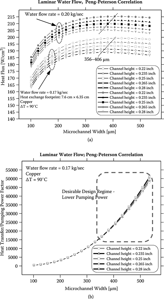
Figure 3.14 (a) Heat flux and (b) heat transfer/ pumping power factor in various water–copper microchannel designs. (Hendricks, T. J. 2008. Proceedings of American Society of Mechanical Engineers 2nd International Conference on Energy Sustainability, Jacksonville, FL, paper no. ES2008-54244. Used with permission from American Society of Mechanical Engineers, New York.)

Figure 3.14(b) shows the effective heat transfer rate to required pumping power ratio, Γ [26], for the same range of microchannel widths and heat exchanger frontal area and footprint assumptions in Figure 3.14(a). It is clear that Γ is increasing sharply in design regions associated with maximum interfacial heat flux and continues increasing sharply at larger microchannel widths, due to smaller pumping powers with simultaneously small decreases in the interfacial heat flux in Figure 3.14(a). This is a highly desirable design regime as the loss in interfacial heat flux can be insignificant as Γ continues increasing sharply. Similarly to Figure 3.13 results, the associated optimum heat flux design regions are significantly influenced by the convective heat transfer correlation used in the analysis and the assumptions and constraints used. Nevertheless, Figure 3.14 and Hendricks [26] show the methodology and approach to microchannel heat exchanger design for TE energy recovery system applications. It is paramount to quantify the heat flux–Γ relationships and design regimes, as well as sensitivities and trade-offs across the entire possible design domain, and uniquely determine optimum heat flux designs and off-optimum design sensitivities to critical design parameters in any given TE system application.

Figure 3.15 shows similar UA–pumping power relationships and heat flux–Γ relationships for a helium gas microchannel heat exchanger design for a constant heat exchanger frontal area and footprint area. Many of the same trends and behavior are exhibited in this gas flow design, as shown in Figures 3.13 and 3.14, except that pumping powers are exorbitantly high and Γ values are therefore quite low in this case for the heat exchanger frontal area and footprint area given. The same, more desirable heat flux–Γ design regimes exist at large microchannel widths. These generally higher pumping powers for gas flow microchannel heat exchanger designs create serious design challenges in TE energy recovery systems, which still warrant further research and engineering work.

Krishnan, Leith, and Hendricks [30] discussed analysis methodologies and design techniques for employing and optimizing microchannel honeycomb designs to enhance gas flow heat transfer in TE systems. This work specifically focused on microchannel designs for automotive heating and air conditioning system applications.

3.3.2.3 Examples of TE/ Microtechnology Integration

There are recent examples [10,11,25,26,30–32] where microtechnology heat exchange technology was investigated or implemented in TE systems. Figure 3.16 displays a recent rectangular honeycomb copper microchannel design that was demonstrated and characterized for a TE cooling system in an automotive application. This particular microchannel heat exchanger design occupied 8 cm × 4 cm × 2 cm in volume and demonstrated low pressure drops (0.52 kPa at ~18 cubic feet per minute air flow) and low thermal resistances near 0.1 C/ W, and it was capable of 250–300 W of thermal transfer at temperature and flow rate conditions consistent with automotive heating and air conditioning requirements [30]. Wang et al. [32] demonstrated successful performance of several microtechnology heat exchangers incorporated within a unique, pioneering hybrid TE–organic Rankine cycle system, which integrated a TE topping cycle with an organic Rankine cycle and vapor compression system to provide simultaneous power production and cooling capacity from a waste-heat-driven source. The TE subsystem used an air microchannel heat exchanger on the hot side and a liquid R-245fa microchannel heat exchanger on its cold side. The organic Rankine cycle operating with R-245fa working fluid used a microchannel heat exchanger for its boiler and recuperator devices [32]. All these microchannel heat exchangers operated stably with low pressure drops and good thermal performance per their design specifications; the organic Rankine cycle (ORC) boiler and recuperator microchannel heat exchangers exhibited actual thermal effectiveness generally above 90%.

Images

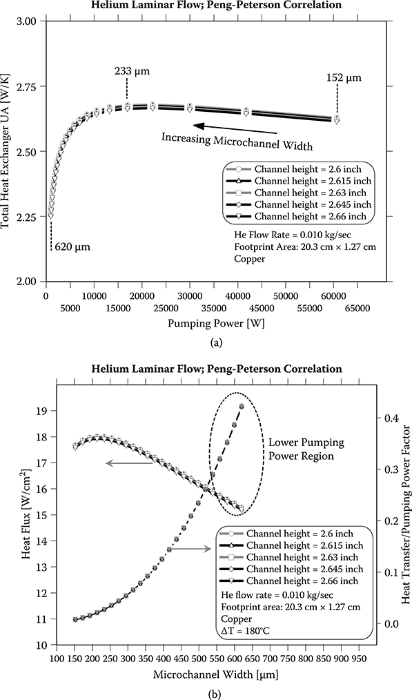
Figure 3.15 (a) Heat exchanger UA and (b) hot-side heat flux in helium flow microchannel designs. (Hendricks, T. J. 2008. Proceedings of American Society of Mechanical Engineers 2nd International Conference on Energy Sustainability, Jacksonville, FL, paper no. ES2008-54244. (Used with permission from American Society of Mechanical Engineers, New York.)

Images

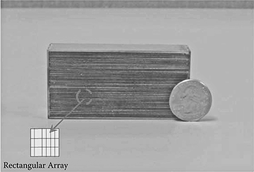
Figure 3.16 Recent rectangular honeycomb microchannel design for TE Systems in automotive application.

There is a common misconception that microchannel heat exchangers necessarily produce high pressure drops and, therefore, have high pumping power. This is not true, as evidenced by the designs in Figure 3.16 and Wang et al. [32]. In fact, if a microchannel heat exchanger is properly designed and properly scaled, its pressure drop need not be any higher than a conventional macrochannel heat exchanger design for a given heat transfer duty and mass flow rate. This also has been shown in numerous examples in Yang and Holladay’s work [33]. The cost of microchannel systems also is being driven down as production volumes increase in potential high-volume applications for automotive and heavy vehicles; industrial processes; residential and commercial heating, ventilation, and air conditioning systems; and power generation.

3.4 Structural Design and Considerations in Thermoelectric Systems

The TE modules in TE heat recovery systems are generally constructed of multiple TE elements that are often bulk elements arranged in an array that is thermally in parallel and electrically in series, as shown in Figure 3.17, or as thin-film elements that encounter a substantial temperature differential across a length dimension perpendicular to and much greater than the thinnest film dimension. The structural design and analysis is a critical aspect of high-temperature thermoelectric heat recovery systems because of thermally induced expansion stresses from materials with even slightly mismatched coefficients of thermal expansion, compression stresses, and tensile stresses developed within the TE elements and module. In bulk element arrays, the TE module is commonly under significant compression of 30 psi up to 200 psi in order to create adequate thermal transport across critical hot-and cold-side interfaces between heat exchanger and TE device surfaces. This compression can be applied at room temperature or the system can be designed to achieve these compressive pressures as it expands to higher temperatures, depending on the details of the design. In thin-film element designs the thermal contact can be supplied compressively also, but often compression is exerted perpendicular to the element length at the element ends in some fashion that is highly design dependent. In any event, the hot side of the TE element can be at temperatures of 600 to 1300 K, while the cold side can be held at 350 to 500 K.

Images

Figure 3.17 Top (a): magnified structural displacements; bottom (b): resulting stresses in a TE module from compressive and expansive forces (displacements in millimeters; stresses in megapascals). Note: The TE hot side is on the top of each element shown.

In addition, the TE elements themselves are electrically connected with a variety of electrically conducting and diffusion barrier materials, which often have different coefficients of thermal expansion from those of the base TE materials. In any event, the combination of compression and thermally induced expansions as the system heats up creates very complex structural displacements and stresses in the TE elements and generates the potential for large structural stresses that can damage the TE element and modules. Figure 3.17 shows a magnified structural displacement map created from a typical structural analysis using the ANSYS^® software package for a typical rectangular parallelepiped TE element/ module design. It highlights how the elements respond to the expansive and compressive forces encountered in the module and in a system. It is not only the TE elements that expand, but the electrical connecting materials and diffusion barrier materials also expand, putting complex tilting and distortion forces on the elements.

As one can see, the TE elements can experience complex expansive displacements and tilting displacements that create complex structural tensile and compressive stresses at various locations in the TE device. Element corners at the rectangular parallelepiped TE device hot side are particularly susceptible to high tensile stresses (i.e., dark regions in the top corner areas), for example, as the device components expand during heating to operational conditions. This fact does not necessarily change whether one is considering a bulk material TE element/ module design as shown in Figure 3.17 or a thin-film TE element/ module design that others have considered in some TE heat recovery applications.

Figure 3.17 exemplifies the type of structural analysis that is required in designing TE elements and modules for thermoelectric heat recovery systems. These element and module structural analyses are generally quite complex and three dimensional in nature. They require strict and comprehensive evaluation of boundary conditions and often require multiple “load steps” as boundary conditions change during fabrication and operation to analyze the TE element, component, and module stresses and displacements properly for all expected environments. The required material properties for performing these analyses are typically Young’s modulus, Poisson’s ratio, coefficient of thermal expansion, and mechanical fracture strengths for each of the materials used for each component in the TE module design. Table 3.4 shows some typical structural property values of common TE materials compared to semiconductors and common metals.

TABLE 3.4 Typical Structural Properties of Common TE Materials Compared to Semiconductors and Common Metals[34, 35]

Images

There are generally no consistent “rules of thumb” or set of equations that one can employ even to get close to accurate structural analysis results. What is generally required is a complete three-dimensional analysis using a general structural analysis code, such as ANSYS^®, COMSOL^®, or other such structural analysis software packages. Furthermore, the TE element and module structural analyses must be tightly coupled with the TE optimization and performance analyses discussed earlier in this chapter to develop optimum, survivable TE element and module designs that satisfy all operational requirements in the environments anticipated for any thermoelectric heat recovery system. For example, in structural analyses exemplified in Figure 3.17, it is often found that longer, thinner TE elements lower the destructive tensile stresses that develop. However, the TE design optimization equations shown in Section 3.2 dictate that longer TE elements will necessarily produce lower power designs. Consequently, requirements for maximizing power output from the TE heat recovery system are in conflict with the requirement to lower structural stresses and ensure TE element and module survival during operational conditions and environments. Therefore, it is imperative that the structural design and analysis be strongly integrated with the thermoelectric and thermal design optimization processes described previously in achieving a truly optimum design for TE heat recovery systems.

3.5 Conclusion

Advanced, high-performance TE energy recovery systems will have a unique and critical role in recovering waste energy in automotive and industrial applications worldwide, with the subsequent benefit of helping to increase global energy efficiency. Optimal design of these systems requires design optimization accounting for three crucial, interdependent design areas: thermoelectric design, thermal design, and structural design. Copious consideration and attention to detail in these three design regimes are equally important to that of obtaining high-performance TE materials in developing TE devices and systems that achieve their full performance potential for these applications. This chapter provides the foundation and methodology for addressing these three critical system design facets and their role in achieving high-performance TE waste energy recovery systems and solutions. If one wants this technology to achieve its full performance potential in future applications, then one must explore comprehensive system design domains using the techniques discussed herein.

Acknowledgments

The authors acknowledge and thank Professor Eldon Case and his group at the Department of Chemical Engineering and Material Science, Michigan State University, East Lansing, Michigan, for their mechanical property contributions in Table 3.4. The authors also thank Mr. Naveen Karri, Engineering Mechanics and Structural Materials Group, Radiological and Nuclear Science and Technology Division, Pacific Northwest National Laboratory, for his support and expertise in preparing critical figures in this chapter. The authors would also like to thank Virginia M. Sliman and Brenda L. Langley at the Pacific Northwest National Laboratory for their rigorous technical editing of this manuscript and their great editorial recommendations.

References

1. Transportation energy data book, ed. 29. 2010. US Department of Energy, Office of Energy Efficiency and Renewable Energy, Vehicles Technology Program. ORNL-6985, Oak Ridge National Laboratory, Oak Ridge, TN. http://cta.ornl.gov/data/index.shtml

2. US Department of Energy, Industrial Technologies Program, Energetics, Inc. & E3M, Inc. 2004. Energy use, loss and opportunities analysis: US Manufacturing and Mining.

3. Hendricks, T. J., and W. T. Choate. 2006. Engineering scoping study of thermoelectric generator packages for industrial waste heat recovery. US Department of Energy, Industrial Technology Program, http://www.eere.energy.gov/industry/imf/analysis.html

4. Hendricks, T. J., and J. A. Lustbader. 2002. Advanced thermoelectric power system investigations for light-duty and heavy-duty vehicle applications: Part I. Proceedings of the 21st International Conference on Thermoelectrics, Long Beach, CA, IEEE catalogue no. 02TH8657, 381–386.

5. Hendricks, T. J. and J. A. Lustbader. 2002. Advanced thermoelectric power system investigations for light-duty and heavy-duty vehicle applications: Part II. Proceedings of the 21st International Conference on Thermoelectrics, Long Beach, CA, IEEE Catalogue no. 02TH8657, 387–394.

6. Crane, D. T., J. W. LaGrandeur, and L. E. Bell. 2010. Progress report on BSST led, U.S. DOE automotive waste heat recovery program. Journal of Electronic Materials 39 (9): 2142–2148.

7. Angrist, S. W. 1982, Direct energy conversion, 4th ed. Boston, MA: Allyn and Bacon.

8. Rowe, D. M., ed. 1995. CRC handbook of thermoelectrics. Boca Raton, FL: CRC Press.

9. Hogan, T. P., and T. Shih. 2005. Modeling and characterization of power generation modules based on bulk materials. In Thermoelectrics handbook: Micro to nano, ed. D. M. Rowe. Boca Raton, FL: CRC Press.

10. Hendricks, T. J., N. K. Karri, T. P. Hogan, and C. J. Cauchy. 2010. New thermoelectric materials and new system-level perspectives using battlefield heat sources for battery recharging. Proceedings of the 44th Power Sources Conference, Institute of Electrical and Electronic Engineers Power Sources Publication, technical paper no. 28.2, pp. 609–612.

11. Crane, D. T. 2011. An introduction to system level steady-state and transient modeling and optimization of high power density thermoelectric generator devices made of segmented thermoelectric elements. Journal of Electronic Materials 40: 561–569.

12. Cobble, M. H. 1995. Calculations of generator performance. CRC handbook of thermoelectrics, Boca Raton, FL: CRC Press.

13. Swanson, B. W., E. V. Somers, and R. R. Heikes. 1961. Optimization of a sandwiched TE device. Journal of Heat Transfer 83: 77–82.

14. Crane, D. T. 2003. Optimizing thermoelectric waste heat recovery from an automotive cooling system. PhD dissertation, University of Maryland, College Park.

15. Crane, D. T., and L. E. Bell. 2006. Progress towards maximizing the performance of a thermoelectric power generator. Proceedings of the 25th International Conference on Thermoelectrics, Vienna, Austria: IEEE, pp. 11–16.

16. Crane, D. T., and L. E. Bell. 2009. Design to maximize performance of a thermoelectric power generator with a dynamic thermal power source. Journal of Energy Resources Technology 131: 012401-1–012401-8.

17. Crane, D. T., and G. S. Jackson. 2004. Optimization of cross flow heat exchangers for thermoelectric waste heat recovery. International Journal of Energy Conversion and Management 45 (9–10): 1565–1582.

18. Sherman, B., R. R. Heikes, and R. W. Ure Jr., 1960. Calculations of efficiency of TE devices. Journal of Applied Physics 31 (1): 1–16.

19. Domenicali, C. A. 1953, Irreversible thermodynamics of TE effects in inhomogeneous, anisotropic media. Physics Reviews 92 (4): 877–881.

20. Mahan, G. D. 1991. Inhomogeneous TEs. Journal of Applied Physics 70 (8): 4551.

21. Skrabek, E. A., and D. S. Trimmer. 1995. Properties of the general TAGS system. In CRC handbook of thermoelectrics, ed. D. M. Rowe, 267–275. Boca Raton, FL: CRC Press LLC.

22. Dughaish, Z. H. 2002. Lead telluride as a thermoelectric material for thermoelectric power generation. Physica B 322: 205–223.

23. Antonova, E. E., and D. C. Looman. 2005. Finite elements for thermoelectric device analysis in ANSYS^®. Proceedings of 2005 24th International Conference on Thermoelectrics, pp. 215–218.

24. Kays, W. M., and A. L. London. 1984. Compact heat exchangers, 3rd ed. New York: McGraw–Hill.

25. Hendricks, T. J., and N. K. Karri. 2009. Micro-and nano-technology: A critical design key in advanced thermoelectric cooling systems. Journal of Electronic Materials 38 (7): 1257–1267, DOI: 10.1007/s11664-009-0709-3, Springer Publishing, New York.

26. Hendricks, T. J. 2008. Microtechnology—A key to system miniaturization in advanced energy recovery and conversion systems. Proceedings of American Society of Mechanical Engineers 2nd International Conference on Energy Sustainability, Jacksonville, FL, paper no. ES2008-54244.

27. Hendricks, T. J. 2006, Microchannel & minichannel heat exchangers in advanced energy recovery & conversion systems. Proceedings of the ASME 2006 International Mechanical Engineering Congress and Exposition, IMECE2006—Advanced Energy System Division. New York: American Society of Mechanical Engineers, paper no. IMECE2006-14594.

28. Incropera, F. P., and D. P. Dewitt. 1990. Fundamentals of heat and mass transfer, 3rd ed. New York: John Wiley & Sons.

29. Liao, S. M., and T. S. Zhao. 2002. Measurements of heat transfer coefficients from supercritical carbon dioxide flowing in horizontal mini/micro channels. Journal of Heat Transfer, Transactions of the ASME 124:413–420.

30. Krishnan, S., S. Leith, and T. J. Hendricks. 2012. Enhanced gas-side heat transfer in rectangular micro-honeycombs. Proceedings of the ASME 2012 6th International Conference on Energy Sustainability & 10th Fuel Cell Science, Engineering and Technology Conference. New York: American Society of Mechanical Engineers, paper no. ESFuelCell2012-91223.

31. Hendricks, T. J., T. P. Hogan, E. D. Case, C. J. Cauchy, N. K. Karri, J. D’Angelo, C.-I. Wu, A. Q. Morrison, and F. Ren. 2009. Advanced soldier-based thermoelectric power systems using battlefield heat sources. In Energy harvesting—From fundamentals to devices, ed. H. Radousky, J. Holbery, L. Lewis, and F. Schmidt (Materials Research Society Symposium Proceedings 1218E, Warrendale, PA, 2010). Paper ID no. 1218-Z07-02. (Proceedings of the Materials Research Society 2009 Fall Meeting, Symposium Z, paper ID no. 1218-Z07-02, Boston, MA, 2009.)

32. Wang, H., T. J. Hendricks, S. Krishnan, and R. Peterson, 2011. Experimental verification of thermally activated power and cooling system using hybrid thermoelectric, organic Rankine cycle and vapor compression cycle. Proceedings of the 9th Annual International Energy Conversion Engineering Conference (Reston, VA: American Institute of Aeronautics and Astronautics, Inc.), paper no. AIAA 2011-5983.

33. Wang, Y., and J. D. Holladay. 2005. Microreactor technology and process intensification. ACS Symposium Series 914, American Chemical Society, Oxford University Press.

34. Hall, B. D., J. L. Micklash, J. R Johnson, T. P. Hogan, and E. D. Case. 2007. A review of mechanical properties for thermoelectric materials. Technical presentation at Materials Science and Technology 2007 Conference, Detroit, MI.

35. Morrison, A. Q., E. D. Case, F. Ren, A. J. Baumann, T. J. Hendricks, C. Cauchy, and J. Barnard. 2012. Elastic modulus and bioxial fracture strength of thermally fatigued hot pressed LAST and LASTT thermoelectric matierals. Materials Chemistry and Physics 134: 973–987.

..................Content has been hidden....................

You can't read the all page of ebook, please click here login for view all page.

Table of Contents for 3 Energy Harvesting Thermoelectric and Microsystems Perspectives and Opportunities and Opportunities

Create new playlist

Sign In

Sign Up

Nomenclature

Table of Contents for
3 Energy Harvesting Thermoelectric and Microsystems Perspectives and Opportunities and Opportunities