
Chapter Two
Energy Positivity and Flexibility in Districts
N. Good
E.A. Martínez Ceseña
P. Mancarella The University of Manchester, School of Electrical and Electronic Engineering, Manchester, United Kingdom
Abstract
This chapter examines the concept of energy positivity and argues that energy positivity, in the classical sense (i.e., districts that generate more electricity than they consume), is not a suitable objective or metric for Energy Positive Neighborhoods (EPNs), or smart energy districts more generally. Instead, it is argued that flexibility is a more suitable objective/metric, given the various variable and dynamic factors which effect electricity systems, and that, in a liberalized system, economic value is the most suitable proxy for flexibility. Through quantitative case studies, the economic value of the classic definition of energy positivity and of flexibility is examined to demonstrate the nonequivalence of these objectives, before suggesting how the economic value metric can be made a better proxy for flexibility. Subsequently, some other possible objectives for an EPN are considered, illustrating how following one objective will generally produce a result which is suboptimal with respect to another metric. Then methods for multicriteria analysis to consider multiple objectives simultaneously are presented, before concluding remarks on energy positivity and flexibility in districts are given.
Keywords
energy positivity
flexibility
distributed energy resources
multienergy
aggregation
district optimization
economic value multicriteria analysis
1. Introduction
Energy positivity is an ill-defined term and potentially subject to controversial interpretations. In the context of a neighborhood (or, equivalently, district), it can be understood to mean “the generation of more electricity, by a neighborhood, than it consumes.” This definition has parallels with the concept of Zero-Energy Buildings (ZEB), or Net-Zero-Energy Buildings (NZEB) (Marszal et al., 2011; Sartori, Napolitano, & Voss, 2012). However, such a simplistic definition needs clarification on several significant points. In existing literature (Sartori et al., 2012; Torcellini, Pless, & Deru, 2006; Reichl & Kollmann, 2011; Marszal et al., 2011), the appropriate metrics, the temporal frame, and the types of energy use to be considered have been identified as key factors in assessment of buildings (and by extension, neighborhoods or districts). These are all certainly relevant for the assessment of an Energy Positive Neighborhood (EPN) also. However, they do not systematically address what may be considered the key defining features of future energy systems. These can be summarized as:
1. increasing penetration of low carbon electricity generation [both variable, such as many types of Renewable Energy Sources (RES), and relatively inflexible, such as nuclear];
2. decreasing availability of traditional, flexible, thermal generators;
3. increasing penetration of electric heating and transport.
These features are significant as they all result in increasing scarcity of a resource which is crucial for the operation of electricity systems, given the need to balance the electricity system second-by-second (i.e., flexibility1). Increasing penetration of low carbon electricity generators will reduce flexibility as they are either nonschedulable as well as partly nondispatchable [e.g., in the case of solar Photovoltaic (PV) and wind generation], or are (traditionally) not designed for frequent and fast modulation (e.g., nuclear). Meanwhile, increasing penetration of large-scale (variable) RES, will increase demand for flexibility at the system level, just as the availability of traditional providers of flexibility (thermal generation) is decreasing. At the same time, increasing penetration of small-scale RES as well as of electric heating and transport is increasing demand for flexible resources at the distribution network level, to prevent voltage and congestion issues (Navarro-Espinosa & Ochoa, 2015; Navarro-Espinosa & Mancarella, 2014; Mancarella, Gan, & Strbac, 2011), which can motivate expensive network reinforcement (Martínez-Ceseña, Good, & Mancarella, 2015). While there are various types of flexible resources available, flexibility from the demand-side, from entities, such as neighborhoods, have been identified as particularly attractive sources (Strbac et al., 2012). Hence, there is clearly motivation for neighborhoods to become, as a primary objective, flexible, rather than energy positive (besides the ambiguity of the terminology itself).
Naturally, given the variable and stochastic nature of demand for energy services (e.g., heating or air conditioning), RES, and plant and networks outages, the demand for operation of flexible resources is variable and dynamic. Hence, to achieve flexibility (rather than energy positivity, in the classic sense) focus should be on strategic adoption of flexible resources and enabling ICT. This motivates methods of neighborhood/district assessment which fundamentally reflect this focus on flexibility. This requirement is, however, not straightforward. The value of flexibility varies substantially, both temporally and spatially, but also according to the preferences of the evaluator. For example, at times of low system demand, flexibility may be important especially in cases when there is little inertia in the system (as it may be in the presence of large volume of power electronics-connected RES). On the other hand, for periods of high system demand, flexibility may have substantial value as the system is more sensitive to shocks due to the increased penetration of inflexible technologies. Similarly, on congested distribution networks with little spare capacity the value of flexibility may be significant to avoid network reinforcement. Finally, whatever the physical status of the electricity system and networks, the value of flexibility may be different to different parties. For example, a consumer with a requirement for high reliability in their electricity supply (e.g., a hospital), may value reliability highly. In contrast, a relatively poor (hence price sensitive) domestic customer may be willing to accept a lower level of electricity supply reliability if this provides a discount on their bill. Similarly, users with an alternative energy-service supply (e.g., back-up electricity generation or an alternative supply of fuel/alternative energy service providing device) may be willing to accept lower electricity supply reliability. In this context, reliability [and to some extent even resilience (Panteli & Mancarella, 2015)] could be provided by flexible neighborhood-level demand-side resources that might respond to economic incentives to decrease their electricity consumption (or increase their production in the case of embedded generation).
Accounting for these varying, dynamic conditions and preferences is not an easy task for one central assessor, making assessment of flexibility difficult. However, in a liberalized system, where (generally variable and dynamic) price signals indicate the value of agent behavior, economic value can be considered the most suitable proxy metric to measure flexibility (Chapter 6). Although it is not a perfect measure, as it relies on well-functioning (i.e., cost-reflective) markets, which may not always be the case, it is the best available. Further its efficacy as a measure of flexibility should only increase as technology increases the penetration of variable, dynamic pricing (Faruqui, Harris, & Hledik, 2010), and reforms (such as including the price of disconnections and voltage reduction in imbalance penalties, and making the penalties reflect the marginal cost of balancing actions) increase the cost reflectiveness of prices (Flamm & Scott, 2014).
Given the identification of economic value as the appropriate proxy measure of the flexibility of a neighborhood, Section 2 examines how the economic value metric of neighborhoods varies given objectives of “classic” energy positivity and flexibility. Quantitative examples demonstrate the material difference in economic value which results from each objective. Section 3 then considers, through further quantitative examples, how optimization of a neighborhood with respect to various objectives which are commonly conflated (i.e., economic value, CO2 emission, and self-sufficiency) are, in fact, not equivalent. Recognizing that decision-makers may want to evaluate neighborhoods according to many criteria, rather than solely according to flexibility, Section 4 introduces the concept of multicriteria analysis, outlining a framework for assessment of interventions according to multiple criteria. Section 5 offers some concluding remarks.
2. Economic Value of an EPN
An EPN will be able to achieve flexibility through exploiting various flexible resources. However, the amount of value will depend on the objective they follow, and the degree to which this objective aligns with the requirements of the system. As explored in more detail in Chapter 6, flexible resources can be classified as storage, substitutable, or curtailable resources (Althaher, Mancarella, & Mutale, 2015). Storage within the EPN can enable the shifting of grid electricity consumption in time. This storage may be of electricity (in the form of a battery or other electrical storage medium), of some other derived energy vector (such as heat in thermal storage), or be of some product within a process (such as clothes within a washing machine) (Zhou, Mancarella, & Mutale, 2016). Substitutable appliances (using an alternative energy vector for fuel) for the provision of the energy service can enable the substitution of one energy vector for another (Capuder & Mancarella, 2014; Mancarella & Chicco, 2013). For example, heat provision may be switched from an Electric Heat Pump (EHP) to a Combined Heat and Power (CHP) unit, resulting in a substitution of electricity with gas (Capuder & Mancarella, 2014; Mancarella & Chicco, 2013), while more general, “multigeneration” cases could also involve cooling (Mancarella & Chicco, 2009). Curtailable resources can, given the willingness of the consumer to put a price on the utility of the energy service that they are consuming, enable the trading of consumer utility (Good, Karangelos et al., 2015; Althaher et al., 2015). For example, pricing thermal comfort would enable optimized trading between thermal comfort and overall utility (Good et al., 2015a). How a neighborhood exploits these resources, and how much economic value they produce, depends on the objective they follow, as shown in subsequent sections.
2.1. Economic Value of “Classic” Definition of Energy Positivity
The “classic” definition of energy positivity is taken here as “the generation of more electricity, by a neighborhood, than it consumes,” also implicitly intending that this electricity should be coming from local resources that bring also environmental benefits (e.g., RES)—even though it may not always be the case. Assuming that a neighborhood will aim to be as (electrically) energy positive as possible, and that measurement is over a year, the objective of an EPN under this definition will be to maximize its net electricity generation, or, equivalently, minimize its net grid electricity consumption, over the year.
With the aim of illustrating the potential effects on economic value associated with pursuing the classic definition of energy positivity, it is useful to consider the effects of employing the three identified sources of flexibility: shifting, substitution, and utility trading. Accordingly, the effects of employing the three types of flexibility will be explored with reference to two notional neighborhoods, situated in the north of England:
• Neighborhood 1 is made of 50 well-insulated flats each heated by an Air Source Heat Pump (ASHP) and each with 1.9 kW of solar PV panels, and a 2 kWh/0.2 kW electrical battery.
• Neighborhood 2 is made up of 50 well-insulated flats each heated by a gas CHP, and each with a 145 L hot water Thermal Energy Storage (TES).
ASHP and CHP are sized according to peak loads (as in Good et al., 2016), resulting in average size of 1.9 kWelectrical for ASHPs and 4 kWgas for CHPs. The ASHPs Coefficient-Of-Performance (COP) varies linearly with the air temperature, taking value of 1.97 at 0°C and 3.51 at 20°C. The CHP is a Stirling Engine type, with thermal efficiency of 0.78, and electrical efficiency of 0.13. Building set temperatures are sampled from a normal distribution with mean 21.6°C and standard deviation of 2.4°C (Shipworth et al., 2010), with set temperatures valid only during times of active occupancy (i.e., the occupants are present and active) (Good, Zhang et al., 2015). The after-diversity peak demands for the neighborhoods are 140 kWthermal and 17 kWelectrical,2 while the annual demands are 231 MWhthermal and 48 MWhelectrical.2
With respect to shifting, as the classic definition of energy positivity is over the period of 1 year, there is actually no benefit from shifting electricity demand/generation, using electrical/thermal storage within daily time scales, as in typical applications. In the case of neighborhood 1 there is no motivation to use any battery storage to shift electricity, as energy positivity is measured over a long period. So, whether the battery storage is employed or not makes no difference considering an objective of energy positivity only. In fact, if the battery is utilized at all the neighborhood will become less energy positive, as battery losses will result in net increase in electricity consumption compared with the no storage case. This inherently disregards the potential economic and environmental benefits that could be accrued by shifting energy consumptions to periods of lower energy prices or carbon intensity.
In the case of neighborhood 2, the objective of maximizing energy positivity provides an incentive to keep the flats at maximum temperature (respecting thermal comfort constraints), to stimulate more CHP operation, and hence more electricity generation. As a result, there is no incentive to match electricity consumption and generation on a settlement period3 by settlement period basis, as energy positivity is defined over the year. To demonstrate how the operation of the energy neighborhood varies when optimized under a classic energy positivity objective, compared with an economic objective, results in this section illustrate the relevant operation of the neighborhood’s resources in terms of CHP electricity production, electricity imports, and TES temperature under both objectives. Here optimization is undertaken for neighborhood 2 on a typical winter day in the United Kingdom. Outdoor temperature (a major determinant of energy demand) and energy prices (not including retailer costs and profit margin, which are socialized over all settlement periods and hence do not produce a time varying signal to drive economic operation of the local resources4) are as in Fig. 2.1 and reflect typical values for the winter period. Settlement periods are half-hourly, as in the UK market.
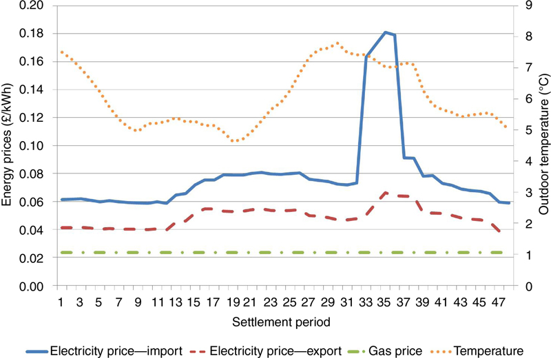
Figure 2.1 Typical winter energy prices and temperatures.
The CHP operation and electricity imports under the classic energy positivity objective are shown in Fig. 2.2, where it can be seen that the storage is not used (indicated by the lack of variation in the TES temperature), with the CHP operation skewed toward the early morning and late evening, when it is colder and there is less active occupancy (and hence no limits on indoor temperature), to try to produce as much electricity as possible, to get as close as possible to “energy positivity” over the day (for the purposes of illustration, energy positivity is enforced in this case over a day rather than a year as in the definition given previously). Alternatively, under an economic objective, the thermal storage would be used more selectively, particularly to better match CHP electricity generation to neighborhood electricity demand (maximizing self-sufficiency in electricity, which could potentially increase economic value by reducing electricity imports during the most expensive periods). The CHP operation and electricity imports optimized based on the objective of minimizing economic costs is shown in Fig. 2.3.
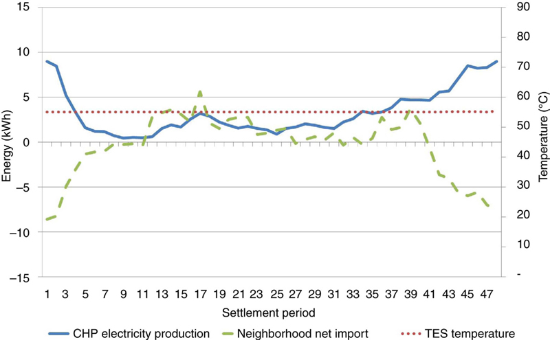
Figure 2.2 Neighborhood 2 behavior under a classic energy positivity objective, typical winter day, United Kingdom.
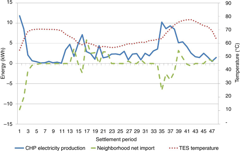
Figure 2.3 Neighborhood 2 behavior under an economic objective, typical winter day, United Kingdom.
An analysis of the key metrics of net energy imports over the day and the relevant costs reveals the misalignment between the classic energy positivity objective and the economic objective, as the energy positive objective produces net imports of −18.7 kWh and costs of £23.75, while the economic objective produces net imports of −12.7 kWh and costs of £22.32.
With respect to substitution, there can be a benefit, in terms of the classic definition of energy positivity, from substituting electricity generating devices for electricity consuming devices (e.g., substituting a CHP for an EHP), or from substituting a nonelectrical device for an electricity consuming device (e.g., a gas boiler for an EHP). Considering neighborhood 1, again on a typical UK winter day, as defined in Fig. 2.1, the addition of a CHP unit may improve energy positivity (according to the classic definition) by substituting EHP heat generation with CHP heat generation, which would reduce electricity consumption. This is demonstrated in Fig. 2.4 which shows the net electricity consumption of neighborhood 1 when heated with EHP heaters or EHP and CHP heaters, under both energy positivity and economic objectives. However, it is important to note that the alternative, to substitute electricity consumption with gas imports, may not increase the economic value of the neighborhood if the electricity price is relatively low compared with the gas price. Under certain conditions (such as low electricity prices due to, for instance, high penetration of PV and wind generation) the electricity price may be such that an increase in energy positivity does not result in energy cost reductions. This is the case in Fig. 2.5 where the addition of the CHP actually increases energy cost under both the energy positivity and the economic objectives. What is worse, of course in this analysis there is no consideration for either environmental assessment (it is possible that fuel substitution increases emissions, which again exposes the criticality of having an ill-defined, electricity oriented definition of energy positivity) or capital investment (attempts to increase electrical energy positivity may result in substantial investment cost that might again make the whole EPN economics shaky).
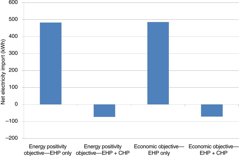
Figure 2.4 Net electricity import under various objectives, with different heating technologies, neighborhood 1, typical winter day.
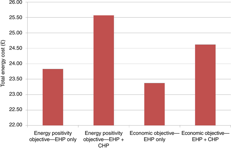
Figure 2.5 Net total energy cost under various objectives, with different heating technologies, neighborhood 1, typical winter day.
With respect to utility trading, energy positivity may be increased by trading utility related to electricity consumption (such as illumination from electric lighting or thermal comfort from electric heating). In effect, this means reducing lighting or heating, to increase energy positivity. In this case the energy positivity and economic objectives coincide, as a reduction in user utility results in both less energy consumption and expense. However, energy positivity could also be increased while increasing supply of some service/commodity, for example, if heating is provided by CHP. In this case, increasing CHP operation will generate additional heat, and hence increasing CHP electricity generation, increasing energy positivity. This is demonstrated by implementing an energy positivity objective on neighborhood 2, again for a typical UK winter day, with a +1°C and a +2°C window around the building set temperature, allowing the temperature to vary freely with the ranges (Tset, Tset + 1°C), and (Tset, Tset + 2°C), where Tset is the building set temperature. As shown in Fig. 2.6, the higher flexibility window allows the buildings’ temperatures to rise as CHP generation is increased to maximize net electricity export (from −17.35 kWh in the +1°C case to −29.40 kWh in the +2°C case). As, compared with gas prices, electricity prices are not high enough for the neighborhood to realize a profit from the increased CHP operation, the cost of energy for the neighborhood rises from £23.65 in the +1°C case to £24.93 in the +2°C case.
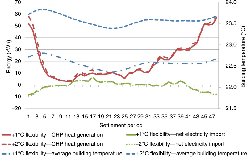
Figure 2.6 Neighborhood behavior with a +1°C and a +2°C flexibility window, typical winter day, United Kingdom.
In order to assess the optimal trade-offs between customer utility and improved energy positivity, it can be attractive to express both utility and energy positivity in widely used and well understood economic terms (Good et al., 2015a). However, using such an approach can be arguable as the value of energy positivity is yet to be understood. In fact, this is a fundamental issue with the classic definition of energy positivity, as discussed insofar: energy positivity, under the classic definition, may have relatively little or no economic value in itself, and therefore is not compatible with a framework which is fundamentally concerned with economic value, as the modern, liberalized energy system is.
In light of this, while, as demonstrated, energy positivity can produce economic value, the extent to which this is true is case specific. Indeed, further to the situations detailed previously, the economic value produced by following an energy positivity objective may be substantially affected by several factors. First, the nature of the imports and exports tariffs to which the neighborhoods are subjected can be central to the economic value of an EPN. In particular, the difference between the imports and exports prices (through a retailer or directly from the market) can be crucial. A wide difference between these prices may increase the economic value of energy positivity if the electricity generation within the EPN is well-matched to its demand (e.g., given CHP utilization). This may be especially true if the neighborhood operates following microgrid principles from an economic standpoint (Good et al., 2016),5 with the neighborhood owning the local electricity distribution network so that flexible resource operation can be coordinated with the objective that most electricity generation is used within the EPN rather than exported,6 besides other potential technical and environmental objectives (Schwaegerl et al., 2011). This is because, commercially, such an arrangement would result in avoidance of substantial imports at high prices that include use-of-system (UoS) charges, as well as avoidance of substantial exports at low prices (although favorable prices may encourage the EPN to export electricity) (Fig. 2.7).
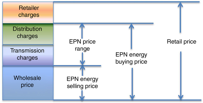
Figure 2.7 EPN selling/buying price.
However, if electricity generation is not well matched to demand (e.g., solar PV without cooling demand, and therefore with higher electricity demand that may occur in mornings or evenings as in the United Kingdom), then a wide difference in imports and exports prices may not significantly increase economic value. This is because electricity would be generated at times of relatively low electricity demand (i.e., the middle of the day, in the United Kingdom; resulting in electricity export at times of low electricity prices), and grid electricity would be consumed at times of low electricity generation (i.e., early mornings and evenings, in the United Kingdom; resulting in electricity imports at times of high electricity prices).
Another factor which may influence the economic value of energy positivity may be the availability of subsidies for low carbon generation. These subsidies tend to encourage renewable but, in most cases, also inflexible technologies, such as PV and wind generation. More pertinently, such subsidies can be applicable to CHP generation, providing incentives to maximize operation, which on the one hand is in line with the electrical energy positivity objective, while, on the other hand, may encourage heat spilling in the case of absence of sufficient local heat demand. Subsidies may be also applicable to (low carbon) EHP heat generation, which may provide a disincentive to energy positivity, by rewarding EHP electricity consumption.
2.2. Economic Value of Flexibility
Following a flexibility objective can be considered to be particularly suitable for the realization of economic value as it recognizes the desirability of increasing use of both local and renewable energy sources, as well as of contributing to the efficiency and security of the wider grid, on which an EPN will rely for electricity imports (when required) and transport of exported electricity. The explicit recognition of these factors is more suited for the realization of economic value as, in a rational, well-designed and liberalized energy system, underlying price signals and incentives are likely to encourage EPN operation in line with increasing local and renewable energy usage and supporting the efficient and secure operation of the grid.
To illustrate how energy price signals can motivate behavior that contributes toward economic value (and therefore toward system efficiency and security), the rationale behind the variable electricity wholesale price signals will be discussed later. Particular emphasis will be placed on the contribution of electricity wholesale price signals to the various components of the energy positivity definition (i.e., local generation, renewable generation, grid efficiency, and grid security).
Generally speaking, electricity prices rise as electricity demand increases, as more expensive plant are brought on-line. High grid prices may motivate the use of cheaper options, such as local flexible generating plant (e.g., CHP). In addition, if prices are expected to remain generally high, this will also motivate investments in local plant, including renewable plant. High grid prices also contribute to grid efficiency and security by motivating operation of demand-side resources [e.g., local generation, storage, and Demand Response (DR)], which can help to maintain system reserves and capacity, thus aiding security and more generally reliability (Zhou, Mancarella, & Mutale, 2015), and avoiding use of inefficient peaking plant, thus aiding efficiency. Low prices may also encourage carbon emissions reductions, as these low grid prices can be due to a substantial amount of renewable generation available in the market. Therefore, increasing grid consumption at these times will boost renewable generation [that may also include electrified heating (Capuder & Mancarella, 2014)], and also aid grid security by avoiding the instability that the combination of low demand and high renewable generation can bring (as more synchronized generators are pushed off the grid).
However, for these price signals to contribute toward the flexibility objective, the price signals must be partially or wholly visible to the EPN (i.e., the retail prices to which the EPN are subject should be dynamic). Under current arrangements, retailers manage all energy trades for EPNs using flat price signals that isolate the neighborhood from the dynamic market price signals. On the one hand, such price arrangements protect EPNs from risks related to price volatility and balance responsibilities. On the other hand, the flat signals obstruct the attainment of the flexibility objective by cutting the EPN off from valuable price signals that would direct the EPN toward desirable behavior. Given the general demonstrated coincidence of flexibility and economic value, such fixed prices also deprive the EPN of the opportunity of employing its flexibility, effectively providing DR (Losi, Mancarella, & Vicino, 2015), to increase its economic value.
Clearly, prices faced by the EPN must be more dynamic for the EPN to achieve flexibility. As also discussed in Chapter 6, this can be achieved by lowering or abolishing regulatory and cost barriers to market participation by small parties, to allow the EPN to partake directly in the relevant markets. In practice, this means deploying a net cost minimization objective, explicitly taking into account price signals from energy markets, ancillary services (such as system reserve) markets, capacity markets/mechanisms, grid fee regimes, low carbon incentive regimes, and taxes. Other solutions, which encourage flexibility but fall short of full market exposure, are also possible. Such solutions may involve a retailer offering more refined retail prices, such as time-of-use, or critical-peak pricing (Six et al., 2015). Such pricing schemes can pass on some of the price signals presented by the various relevant markets, while ensuring some protection and predictability for the EPN. However, such schemes will also tend to reduce the degree of flexibility, and hence economic value available to the EPN (compared to full exposure to markets). This is because, while risk is correlated with price dynamism (more dynamic prices mean more risk), so is potential value (more dynamic prices offer more potential value) for those parties with the necessary flexibility and optimization and communication capabilities (as demonstrated in the COOPERaTE project). This relationship between risk and potential reward is illustrated in Fig. 2.8.
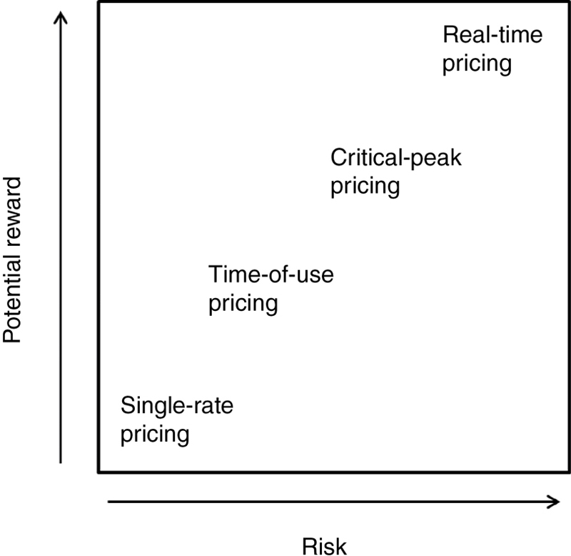
Figure 2.8 Risk and reward (for the EPN) of various pricing schemes.
To demonstrate how dynamic prices can motivate behavior more in-line with the flexibility objective, the optimal CHP electricity generation regime subject to retail and dynamic prices7 is further analyzed for neighborhood 2 (Section 2.1) on a typical UK winter day (Fig. 2.9). Fig. 2.9 shows how visibility of dynamic prices, which directly reflect the prices in the various applicable markets, encourages shifting CHP operation as much as possible (given the limited flexibility afforded by the associated hot water thermal energy stores) toward times of high price. This reaction to price signals results in a reduction of total energy cost from £13.80 when the operation of CHP is optimized based on retail signals to £12.68 when CHP is optimally operated based on dynamic prices.
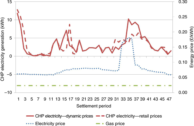
Figure 2.9 Neighborhood CHP electricity generation under retail and dynamic prices.
2.2.1. Further Aligning of Flexibility and Economic Value Objectives
Besides becoming exposed, to a greater or lesser extent, to the various market price signals, for maximum efficacy in pursuing the flexibility objective it is necessary that market designs and the designs of regulated charging regimes (such as for grid fees) are in line. That is, that they encourage local and renewable generation, grid efficiency, and system security.
Based on the aforementioned, for example, recognition of the benefits of local generation (e.g., reduced losses, increased reliability, and lower carbon emissions), in the form of payments or grid fee rebates, would further encourage the local generation component. An increased carbon price would similarly encourage grid-level renewable generation (given the low-carbon status of renewable generation). Extending the carbon market to the local level, or increasing subsidies for local small-scale renewable (electricity and heat) generation would also encourage the renewable component at the local level. With respect to grid efficiency and system security, several measures could be taken to further align the proxy economic value objective with the true flexibility objective. Capacity markets or mechanisms could be introduced (if not already in place) to motivate cost–effective supply adequacy (Zhou et al., 2015), and the design of system frequency response and reserve products could be tailored to remove barriers to demand-side resources, such as may be found in an EPN. At the local level, efficient and secure operation may be encouraged and aligned with the economic objective through incorporation of a Distribution Network Constraint Management (DNCM) service (Chapter 6), and through monetization of the benefits of the EPN concept in terms of increased reliability (brought, e.g., through implementation of microgrid capability) (Syrri, Martínez-Ceseña, & Mancarella, 2015; Schwaegerl et al., 2011). At both transmission and distribution levels, grid fees could improve grid efficiency and security by becoming more cost reflective and, thus, recouping more network costs at times of highest network stress (i.e., from customers whose operation results in network stress) (Martínez-Ceseña et al., 2015).
3. Alternative Objectives/Criteria
Although the focus in this chapter has been on discussing the key advantages associated with maximizing the flexibility inherent in energy neighborhoods, it is of interest to consider that this objective is only one of the many objectives that may be pursued (Schwaegerl et al., 2011). For example, a neighborhood may wish to follow a specific CO2 minimization objective in order to burnish their green credentials. This would result in increased operation of flexible low-carbon plants such as CHP, employment of storage to better match demand to low-carbon generation (to shift grid consumption to low-carbon periods) and, possibly, trading of utility at high-carbon times. Alternatively, a neighborhood may wish to follow a local energy utilization maximization objective. This will involve matching local generation to local demand as much as possible, without regard to prices or CO2 emission rates. This would result in increased operation of local flexible plants, such as CHP or diesel generators, and operation of any storage to assist in matching local generation and demand.
However, it is important to note that while the aforementioned objectives may motivate economically valuable behavior, given the general coincidence of economic and low-carbon drivers (i.e., high CO2 generation is often expensive), and of economic and local energy drivers (as on-site generation avoids UoS costs and can avoid some elements of taxation), pursuing a noneconomic objective may result in a suboptimal economic value for the EPN.
To illustrate this, consider as an example that the operation of neighborhood 2 is optimized for a typical winter day with respect to three different criteria, which could be the criteria of an employed energy optimization engine (such as that explored in Chapter 4):
1. minimize CO2 emission (both local and grid);
2. maximize local energy utilization (self-sufficiency); and
3. maximize economic value.
The neighborhoods are optimized for a typical winter day, with energy price and grid CO2 emission rates (based on the UK context) as in Fig. 2.10.
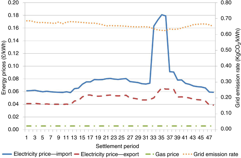
Figure 2.10 Energy prices and grid emission rate, typical winter day.
For each case, the relevant CO2 emission (including both local and grid emissions), the amount of energy traded with the grid (as a measure of neighborhood self-sufficiency) and the total energy cost are quantified. The results for the three studies are shown in Table 2.1.
Table 2.1
Optimization results, neighborhood 2
| CO2 emission (kg) | Cost (£) | Grid usage (kWh) | |
| Economic value maximization | 241.34 | 22.24 | 72.21 |
| CO2 emission minimization | 225.06 | 22.56 | 22.08 |
| Self-sufficiency maximization | 227.06 | 22.78 | 20.00 |

Results in Table 2.1 clearly highlight that while some optimization criteria may produce results which are desirable with respect to other metrics, a result will be generally suboptimal with respect to a given criteria unless it is optimized specifically with respect to that criteria.
More detail is shown in Figs. 2.11–2.13, which show CHP electricity generation, local and grid CO2 emission, and energy cost in the cases of optimization with respect to economic value, CO2 emission, and self-sufficiency, for neighborhood 2, respectively. As shown through comparison of Figs. 2.11 and 2.12 the profiles for CO2 minimization and self-sufficiency maximization are quite similar, as both the CO2 minimization and self-sufficiency maximization objectives are served by minimizing imports from the grid. The slight difference arises as CO2 emissions are minimized by directing grid consumption to a later period, where grid emission rates are lower. In contrast, the grid is used more often when maximizing economic value, as although there are penalties associated with grid usage (as UoS fees and taxes are charged on import, but not accrued as profits during export), these do not produce as high an incentive as in the previous cases to avoid electricity imports (and hence export, during other periods). The relationship between electricity prices and grid emission rates means that operating the neighborhood based on optimal economic gain also produces reasonably low emissions (as the CHP is motivated to operate at high price times, reducing the neighborhood grid consumption and hence grid emissions). It is worth noting that a neighborhood primarily heated by EHP would have a different result, as correlation of high grid emission rates and low prices would motivate consumption at times of high grid emissions.
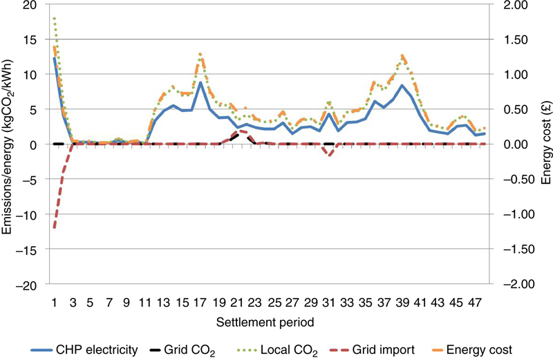
Figure 2.11 Neighborhood 2 behavior, CO2 minimization case.
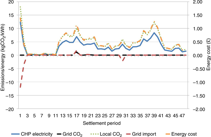
Figure 2.12 Neighborhood 2 behavior, self-sufficiency maximization case.
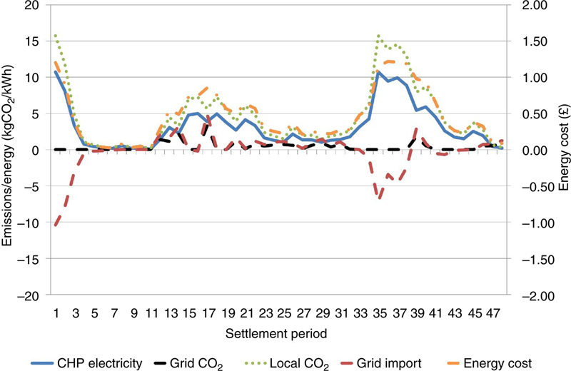
Figure 2.13 Neighborhood 2 behavior, economic value maximization case.
4. Multicriteria Analysis
In practice, parties are likely to be interested in several criteria (such as economic value, CO2 emissions, or self-sufficiency, as in Section 3) when assessing an intervention such as a new operational regime for the neighborhood, installation of CHP or TES units, and so forth. In the planning phase of an EPN, a multicriteria analysis can be undertaken to assess the suitability of an intervention, considering various criteria. This may be useful when an investor wants to assess and compare interventions according to several metrics at once, such as the CO2, energy positivity, and cost metrics in Section 3. For this purpose several techniques are available, such as the direct analysis, linear additive model, and hierarchy method, among others (Zopounidis, Pardalos, & Fallis, 2010). The outcome of a multicriteria analysis is the identification of an intervention that is deemed to perform better than the rest with regard to all criteria (a ranking of the projects may also be possible). The development of a multicriteria Cost Benefit Analysis (CBA) is particularly relevant for this work, as EPNs may want to follow various objectives and assess interventions according to various economic, environmental, and energy criteria. This section briefly overviews classical multicriteria analysis techniques that may be used for the assessment of the EPN concept. For such purpose, a small illustrative example is presented, on assessment of intervention options.
A multicriteria CBA is meant to compare different intervention options based on relevant criteria. In the context of this book, the interventions may represent a vision of the EPN (e.g., investment in particular infrastructure and provision of a specific portfolio of services) from the perspective of an actor (e.g., consumers, retailers, and so forth) under a given market framework. For this purpose, it is convenient to present the performance of the interventions according to different criteria in the form of a matrix (performance matrix) as shown in Table 2.2. In the examples later, performance criteria include Net Present Value (NPV), payback time, Internal Rate of Return (IRR), and CO2 emissions.8 The performance of each intervention option has, for illustration purposes, been set arbitrarily and, for the sake of simplicity, each criterion is expressed as either attractive or unattractive. In practice, each particular criterion would typically be assigned a numerical value.
Table 2.2
Example of a multicriteria performance matrix
| Intervention | NPV | Payback time | IRR | CO2 emissions |
| Option A | Attractive | Attractive | Attractive | Attractive |
| Option B | Unattractive | Attractive | Attractive | Attractive |
| Option C | Attractive | Attractive | Unattractive | Unattractive |

The basic technique (and thus first step) to perform the multicriteria analysis is direct analysis. Direct analysis consists of inspecting if any of the options performs as well or better than all the other options according to each criterion. In this example, this would be option A, which is attractive according to all criteria under consideration. That is, this option offers high benefits (high NPV) on the short term (low payback times), high premium for the capital invested (high IRR) and low environmental impact (low CO2 emissions), all of which are attractive for the corresponding criteria. In practice, there might not be an option that meets the direct analysis requirements, thus other multicriteria techniques have to be used.
If it can be reasonably assumed that all criteria are independent of each other (e.g., the perception of the NPV will not change regardless of the payback time) and can be assigned a weight, the linear additive model may be applicable for the analysis. This technique consists of assigning a weight to each criterion and multiplying the score of each project by the weight. This would produce a single criterion for each intervention option based on which the best alternative can be determined. Such an approach can also be used to form a multicriteria objective, in the operational domain. Such an objective could be used to weight the economic value, CO2 and self-sufficiency objectives discussed in Section 3. In order to illustrate this, assume that each option is credited 1 point per criterion if its performance is attractive. Accordingly, option B is worth 3 points (for its performance according to the payback time, IRR, and CO2 criteria) and is deemed a better alternative than option C, which would only be credited 2 points (for its performance according to the NPV and payback time criteria), while option A would be deemed the best option given its 4 points (for its performance according to all criteria). Clearly the weight assigned to each criterion is a key parameter, as it has significant impact on the outcome of this technique.
Now, if it is not reasonable to assume that all criteria are independent of each other (e.g., a high NPV is desired but short payback times are preferred) an analytical hierarchy process could be used. In this case a pairwise comparison approach (based on a particular analysis or judgment) is used to determine the proper weights for the different criteria and intervention options. In order to illustrate this process, consider the pairwise weights shown in Table 2.3. Table 2.3, which illustrates how a given criterion (row) is valued with respect to other criteria (column) (e.g., the NPV criterion is deemed twice as valuable as the IRR criterion and thrice more valuable than the CO2 emissions criterion).
Table 2.3
Example pairwise weight for the different criteria
| NPV | Payback time | IRR | CO2 emissions | |
| NPV | 1 | 0.5 | 2 | 3 |
| Payback time | 2 | 1 | 1 | 2 |
| IRR | 0.5 | 1 | 1 | 2 |
| CO2 emissions | 0.333 | 0.5 | 0.5 | 1 |

The weights for each criterion associated with the example of pairwise comparison are presented in Table 2.4. As it can be seen, the payback time is deemed the most valuable criterion, followed by the NPV, IRR, and CO2 emissions. An explanation of the mathematics required to process this matrix to obtain the weight for each criterion is beyond the scope of this chapter. It will only be mentioned that the weights can be determined as the eigenvector associated with the maximum eigenvalue of the matrix (for more information, see Weisstein, 2016).
Table 2.4
Criteria weights according to an analytical hierarchy process
| Criterion | Weight |
| NPV | 0.31 |
| Payback time | 0.34 |
| IRR | 0.23 |
| CO2 emissions | 0.12 |
Following the weighting procedure undertaken previously, a similar procedure is performed for the assessment of the intervention options. For the sake of simplicity, option A is not considered in this weighting procedure (as it would be deemed the best in this analysis due to its attractive performance according to all criteria) and an investment option is deemed twice as valuable as another if its performance under a given criterion is better according to Table 2.2. The results of such a pairwise comparison and the associated weights are shown in Tables 2.5 and 2.6, respectively.
Table 2.5
Pairwise comparison of intervention options
| Options | NPV | Payback time | IRR | CO2 emissions | ||||
| B | C | B | C | B | C | B | C | |
| B | 1 | 0.5 | 1 | 1 | 1 | 2 | 1 | 2 |
| C | 2 | 1 | 1 | 1 | 0.5 | 1 | 0.5 | 1 |

Table 2.6
Example intervention option weights according to an analytical hierarchy process
| NPV | Payback time | IRR | CO2 emissions | |
| Option B | 0.33 | 0.5 | 0.67 | 0.67 |
| Option C | 0.67 | 0.5 | 0.33 | 0.33 |

Finally, the weights for both criteria and intervention options are combined (i.e., the sum of the weight of the option multiplied by the weight of the corresponding criterion). The results show that option B is marginally a better option than option C under the selected criteria and weights (Table 2.7).
Table 2.7
Results for the example according to an analytical hierarchy process
| NPV: 0.31 | Payback: 0.34 | IRR: 0.23 | CO2: 0.12 | Ranking | |
| Option B | 0.33 | 0.5 | 0.67 | 0.67 | 0.51 |
| Option C | 0.67 | 0.5 | 0.33 | 0.33 | 0.49 |

In cases where district assessors are interested in multiple assessment criteria, such as energy positivity and flexibility, but extensible to any other criteria (such as CO2 emissions and economic value, as discussed in Section 3), the methods presented here are clearly useful, in the EPN planning phase. Further, the linear additive model (in which criteria are assigned weights equaling unity) may be employed for operational optimization. This may enable simultaneous consideration of multiple criteria (such as economic value, CO2 emissions, and self-sufficiency, as in Section 3). In all cases, assessors must determine the weights that should be assigned to various criteria. Assuming districts are primarily concerned with minimizing costs, most weight is likely to be given to the economic objective. Thus, if price signals can be considered an effective indicator of the value of flexibility, economic value is demonstrated to be a suitable proxy for flexibility (Section 1).
5. Conclusions
This chapter has introduced the concept of flexibility (of energy resources) as an alternative to the inflexible, static, classical concept of energy positivity for a neighborhood. The key defining features of future energy systems (which both decrease the availability of flexibility in the electricity system, and increase the demand for it) have been reviewed, and the demand for flexibility, and hence its value, was shown to be varying and dynamic. Furthermore, the preferences of consumers (specifically in relation to electricity supply reliability) was also shown to be varying and dynamic, increasing complexity, as such changing preferences mean that the value of flexibility varies not only spatially and temporally, but also by individual. The economic value of both the classical energy positivity definition and of flexibility was demonstrated through quantitative case studies. In these case studies the result of using flexible resources (i.e., storage, substitutable and curtailable resources) to pursue an energy positivity objective and an economic (flexibility) objective was presented. In particular the nonequivalence of the two objectives was demonstrated. Subsequently, measures that would further align the flexibility and economic objectives, to ensure the economic objective better motivates behavior beneficial to the system, are reviewed. Possible alternative objectives and criteria were then examined, and the general principle that optimization with respect to one objective will result in behavior which is suboptimal with respect to other criteria was asserted, again through quantitative case studies. Methods for multicriteria analysis of interventions, for use when assessors need to balance the multiple, possibly competing, objectives in the EPN planning phase were then presented.
Through development and explanation of the concept of flexibility, comparison to the inflexible, static, classical definition of energy positivity, and through quantitative studies, this chapter demonstrates the suitability of flexibility, and, indeed, the inadequacy of the concept of energy positivity, especially when ill-defined and focused on the electrical side only, as measures of desirable behavior in current and future electricity systems. However, in a power system context, the key message is that the value of energy services and electricity supply reliability varies by individual, and that the value of demand and generation, and hence system and network redundancy, vary in time and space. Hence, neighborhoods should be optimized and assessed using objectives and metrics which reflect this. Naturally, this requires suitable models and optimization algorithms (as detailed in Chapter 4) and suitably advanced ICT for monitoring, communication and to undertake complex optimization (Chapter 5). Another key message is that, in the absence of any other practical objective/metric, economic value should, in a liberalized electricity system, be used as a proxy for flexibility. Further, this objective/metric can be made a better proxy through improving the cost reflectivity of prices. In this context, economic value should be assessed through quantification of the district business case, which is discussed in detail in Chapter 6.
..................Content has been hidden....................
You can't read the all page of ebook, please click here login for view all page.