
Simulation Tools and Optimization Algorithms for Efficient Energy Management in Neighborhoods
Abstract
In this chapter different schemas for energy optimization in Neighborhoods are presented in detail and a Modelica-based library is used to represent the dynamics of Neighborhood Energy Systems and their interactions. The scalability of the library allows to efficiently simulate city districts.
Keywords
1. Introduction
1.1. Motivation
1.2. Our Contributions
2. Preliminaries
Table 4.1
Thermal and electrical generation, storage, and consumption considerations
| Electrical | Thermal | |
| Generation | Adjustable (variable): • CHPs
• Fuel cells
Nonadjustable (parameter): • Wind turbines
• PV cells
|
Adjustable (variable): • Heat pumps
• CHPs
• Gas boilers
Nonadjustable (parameter): • Solar thermal heating
|
| Storage | Battery | Water tank storage PCM storage |
| Consumption | Electrical Load profiles | Thermal Load profiles |
| Network | Electrical connection | Thermal loop |


3. Simulation Models for Energy Positive Neighborhoods
3.1. Time Constants
3.2. Modeling Language
Table 4.2
Available energy components of COOPERaTE demonstration sites
| Feature | Data requirements and parameters | Challenger | Bishopstown |
|
Building physics |
|||
| Walls | Wall structure | ✓ | ✓ |
| Floors | Floor and piping plan | ✓ | ✓ |
| Windows | Insulation standards | ✓ | ✓ |
|
Heating system |
|||
| Boiler | Technical specifications | ✓ | ✓ |
| Combined Heat and Power (CHP) | Technical specifications | ✓ | ✓ |
| Solar thermal panel | Technical specifications | ✓ | ✓ |
| Heat Pump (HP) | Technical specifications | ✓ | ✓ |
| Storage | Technical specifications | ✓ | ✓ |
| Radiator | Technical specifications | ✓ | ✓ |
|
Electrical system |
|||
| Grid | Topology, Cable type and Load profiles | ✓ | ✓ |
| Battery storage system | Total capacity and Power of interface converter | ✓ | ✓ |
| Photovoltaic (PV) installations | Total installed power and area, Location, Temperature data, Solar irradiation data | ✓ | |
| Electric Vehicle (EV) charging stations | Charging type and power | ✓ | |
| Wind Turbine | Rated power, Technology and Wind velocity data | ✓ | |

3.3. Thermal System
3.4. Electrical System

3.5. Model Library
3.5.1. Thermal Components
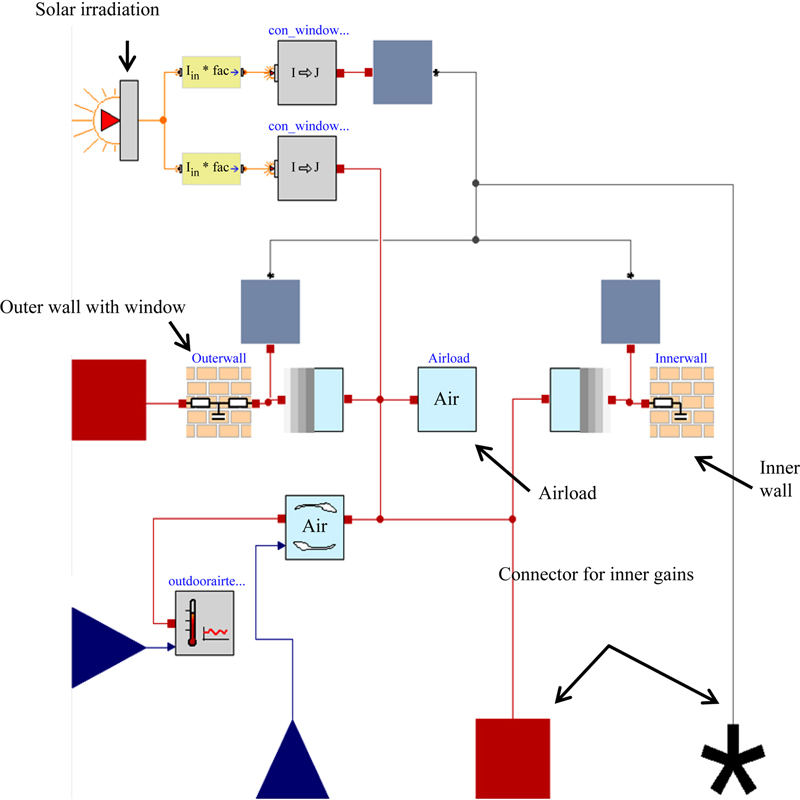
3.5.1.1. Thermal Zone Model and Building Physics
| Description | The building physics library comprises all relevant components to represent a building through a simulation model. Basic components are outer and inner walls, air exchange, equivalent air temperature, solar irradiation gains, and radiation exchange. Based on these components a reduced multizone model of a random building can be built which also contains heat exchange interfaces, that is, radiators that represent the connection between the building mass and enthalpy flow within the building. The thermal connection to external heat generation and storage facilities is achieved via enthalpy connectors. |
| Parameters | Inner and outer walls • Initial temperatures (°C)
• Resistance (K/W)
• Heat capacity (J/K)
• Area of walls/floors (m2)
• Heat transfer coefficient [W/(m2 K)]
• Emissivity (−)
|
Windows • Factor for convective part of radiation through windows
• Window area (m2)
• Emissivity (−)
• Energy transmittance (−)
Room air load • Volume of air in zone (m3)
• Density of air (kg/m3)
• Heat capacity of air [J/(kg K)]
|
|
| Interfaces |
• Total solar irradiation (beam and diffusive)
• Weather (Real Input)
• Infiltration temperature (Real Input)
• Ventilation infiltration (Real Input)
• Internal gains (Real Input)
|
| Formulation | The thermal zone model is based on the simplified control engineering model which is described in the German VDI 6007 standard. The basic idea behind the previously mentioned model is the equivalence between the differential equation of the thermal conduction in a wall and the processes in an idealized electrical cable, as shown in the following equation:
where T is the temperature, R is the thermal resistance of the wall layer, and C is the heat capacity of the wall layer. According to the norms 6007 and 6020 individual building components can be divided into three basic groups: • Outside surfaces, such as external walls, roof, outside, windows, etc.
• Internal walls for which the temperature conditions and radiation conditions prevailing in the adjoining rooms are practically equal (adiabatic loading).
• Internal walls which adjoin rooms with different temperature and radiation conditions, such as a cellar.
The different wall types can be modeled using the equivalence explained earlier, leading to a 2-transfer functions model of a thermal zone, depicted in Fig. 4.5. The resistances and capacities of the walls are calculated depending on the wall’s structure and its geometry. The model representation of a thermal zone in Modelica according to VDI 6007 is shown in Fig. 4.6 (Lauster, Streblow, & Müller, 2012). |


3.5.1.2. Boiler
| Description | The Boiler component is a model of a gas or oil boiler, which—depending on the parameterization—can be operated as a conventional or condensing boiler. It increases the enthalpy of the passing medium by raising its temperature and calculates the fuel consumption according to the current boiler efficiency. The model is table based and internally controlled by a PID controller, which controls the flow temperature that is externally prescribed by a heating curve. This boiler model is able to perform a modulated operation in which the range is determined by parameters. These parameters will be taken either from manufacturer specifications or measurement data. The model is able to represent boilers of different kinds and sizes with appropriate parameters. |
| Parameters |
• Initial temperatures (°C)
• Water volume inside the boiler (m3)
• Nominal heating power (W)
• Modulation rage (%)
• η Efficiency depending on flow temperature and boiler load (−)
• PID controller factors (−)
|
| Interfaces |
• Set flow temperature (Real Input)
• On/Off switch (Boolean Input)
•
|
| Formulation | The heating medium which flows into the component via the enthalpy connector is heated up to the prescribed set temperature by an ideal heating element. The thermal output
|

3.5.1.3. Heat Pump
| Description | The heat pump component is a model suitable for both air and ground source heat pumps. It increases the enthalpy of the passing medium by raising its temperature. Additionally, the power consumption is calculated. Since it is a table-based model, the coefficient of performance (COP) of the heat pump is not influenced by the type of ambient energy source, but its temperature. The source is idealized as an infinite energy source with an externally prescribed temperature (outside air or brine temperature). The heat pump is able to modulate in a defined range. The necessary table data will be taken from the manufacturers’ or measurement data. Depending on the parameterization the heat pump represents an air-to-water or brine-to-water heat pump in a system simulation environment. The connection to the electrical system is achieved through the electrical power consumption output which is used to formulate the relation between voltage and current. |
| Parameters |
• Initial temperatures (°C)
• Modulation range (%)
• PID controller factors (−)
• Start-Up and Shut-Down time (s)
•
• Electric Power table (W)
|
| Interfaces |
• Source temperature (Real Input)
• Sink temperature (Real Input)
• Ntarget Target compressor speed (Real Input)
• On/Off switch (Boolean Input)
• COP Current COP (Real Output)
• Pel,max Electrical power consumption (Real Output)
|
| Formulation | The externally prescribed target compressor speed of the heat pump determines the load state. With the source and sink temperatures as environmental status the maximum condenser heat flow and the corresponding power consumption are delivered by two separate tables. Based on these values the actual COP and thermal output
|


3.5.1.4. CHP Generator
| Description | The CHP generator component is a model of a combined heat and power generator with two enthalpy ports, which increases the enthalpy of the passing medium by raising its temperature. Additionally, the generated electrical power is calculated as an output of the model. It can be operated in a heat or power driven mode. Depending on the operation mode a power/heat input signal is used to determine the current generation status. The model is based on empirical data and the produced power and heat are calculated internally with a polynomial formula for which the weight factors must be provided either by the manufacturer or can be determined through the analysis of measurement data. The model’s purpose is the representation of a CHP in a multiphysics energy system simulation. The connection to the electrical system is achieved through the electrical power input which is calculated from the voltage and current information at the connection point. |
| Parameters |
• Pel,max Maximum power output (W)
• Maximum thermal output (W)
• Modulation range (%)
• ai
,bi
Polynomial weight factors/coefficients
• Control mode (heat or power driven)
• Internal heat capacity (J/K)
|
| Interfaces |
• Electrical power (Real Input)
• Thermal power (Real Input)
• Operation mode (Boolean Input)
• On/Off switch (Boolean Input)
• Electrical power (Real Output)
• Thermal output (Real Output)
• Gas/fuel consumption (Real Output)
|
| Formulation | At first the electrical and thermal efficiencies ηel and ηth are calculated depending on the coefficients of the polynomial, the maximum electrical power output, medium mass flow rate
Depending on the generation mode (heat or power driven) the current thermal and electrical output power is calculated using the power/heat demand input signal and the efficiencies. Based on the output flows and the efficiency, the gas consumption
|


3.5.1.5. Solar Thermal Panel
| Description | The solar thermal panel model has two enthalpy ports and increases the enthalpy of the passing heating medium by raising its temperature. The beam and diffusive irradiation from the environment is collected by the panel and then transferred to the heating medium within the device. The efficiency of this transfer is mainly influenced by the temperature difference of the heating medium and the environmental air. |
| Parameters |
• Reference efficiency of the collector (−)
• Heat exchange coefficient with the environment [W/(m2K)]
• Apanel Panel area (m2)
• Incident angle modifier (−)
• Panel location and orientation
• Ground reflection coefficient (−)
|
| Interfaces |
• Ta Environmental air temperature (Real Input)
• Beam and diffusive radiation (Real Input)
|
| Formulation | Using the input radiation, orientation, and location data, the total radiation on the tilted panel surface G can be calculated. The thermal efficiency η can be calculated depending on the difference between the mean panel temperature Tm and the environmental air temperature with polynomial coefficients ai
which are either given by the manufacturer or determined empirically. Hereby the total thermal output of the panel
|


3.5.1.6. Thermal Storage
| Description | The thermal storage model represents a stratified water storage tank, where the stratification is achieved by the implementation of n discrete layers. Buoyancy flow within the tank is also considered. The number, position, and type (heating coil/direct flow) of the load and unload cycles can be defined as a parameter. Additionally, the tank volume and insulation is fully adjustable, enabling the model to represent random hot water storage tanks. |
| Parameters |
• Number of discrete layers (−)
• Medium density (kg/m3)
• Medium specific heat capacity [J/(kgK)]
• Thermal conductivity of medium [W/(mK)]
• Inner and outer heat transfer coefficient [W/(m2K)]
• Tank and coil measures
|
| Interfaces |
• Layer temperature (Real Output)
|
| Formulation | The enthalpy connectors for loading and unloading the storage tank are, depending on their position, connected to a particular discrete layer of the tank or a coil inside the tank. For the case of tank loading the function of the tank can be described as follows. The enthalpy of a passing medium is to a certain extent transferred from the medium to the layers through which it flows or to the layers which are connected to the corresponding heating coil. After passing the predefined layers of the tank or the heating coil, the medium leaves the storage tank with a certain enthalpy difference which is transferred to the internal storage medium. The layers itself are also connected to each other. The exchange of enthalpy between these layers occurs on the one hand by simple heat conduction
These different heat flows also depend on the height of each discrete volume hlayer and their lateral and front surface area Alayer,front and Alayer,lateral respectively:
The unloading process of the storage tank is vice versa. |


3.5.1.7. Heat Exchanger
| Description | The heat exchanger component is a model of a plate heat exchanger with n × 2 discrete volumes. It has two enthalpy input and output connectors each and is fully adjustable in size, discretization, and material. The purpose of this component is to enable heat transfer between two different mediums that are not allowed to be in direct contact/mixture, for example, heating water and solar thermal fluid (Fig. 4.7). |
| Parameters |
• Number of discrete volumes (−)
• Total heat exchanger volume (m3)
• Total heat exchanger plate area (m2)
• Heat exchanger heat transmission coefficient [W/(m2K)]
|
| Interfaces |
• None
|
| Formulation | The discrete volumes of the heat exchanger are arranged in an alternating manner. Thus, each volume containing the hot medium is neighboring a volume containing the cold medium. Those neighboring discrete volumes are thermally connected to each other by a heat transfer component. Based on the heat flow between the individual volumes
|


3.5.1.8. Radiator
| Description | The radiator component is a model of a hot water radiator. It has two enthalpy ports and is fully adjustable in size, discretization, and material. The purpose of this component is to enable heat transfer between the circulated heating medium, mostly water, and the room airload described in Section 3.5.1.1. |
| Parameters |
• Nominal heating power (W)
• Number of discrete volumes (−)
• Geometric measures (m)
• Material properties of the radiator
|
| Interfaces |
• None
|
| Formulation | The heat
|

3.5.1.9. Pump
| Description | The pump component is a model of an ideal pump, which creates a prescribed heating medium mass flow between enthalpy connectors. It is also used for the type declaration of the heating medium. Since the pump can ideally prescribe a mass flow rate, conventional throttle valves are not necessary for a system setup. |
| Parameters |
• Specific heat capacity [J/(kg K)]
|
| Interfaces |
• Heating medium mass flow rate (kg/s)
|
| Formulation | The pump component simply prescribes the mass flow
|

3.5.1.10. Three-Way Valves
| Description | The three-way valve model is able to represent either a distribution or a mixing valve. As a distribution valve it splits a mass flow
Used as a mixing valve two separate mass flows
Since the pump (Section 3.5.1.9) can ideally prescribe a mass flow rate, conventional throttle valves are not necessary for a system setup. |
| Parameters | Three-way valve type (distribution/mixing) |
| Interfaces |
• Valve opening position
|
| Formulation | The mass flows and enthalpies of each enthalpy connector for the distribution/mixing valve are calculated as follows: Distribution valve
Mixing valve
|


3.5.2. Electrical Components
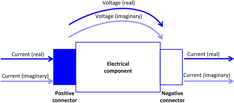
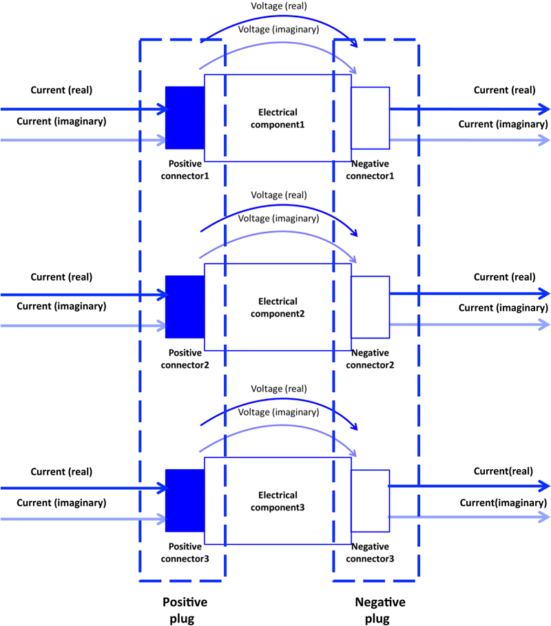
3.5.2.1. Electrical Line
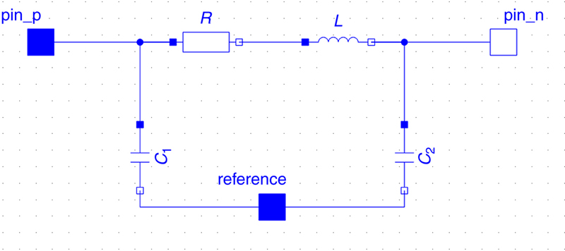
| Description | The electrical line model represents effects which cable properties introduce in electrical systems in low voltage and medium voltage, as opposed to ideal connections in which no losses or capacitive and inductive effects occur. It has three pins: the positive and negative pin as well as a reference pin which may be connected to ground or any other reference point the user would like to choose (Fig. 4.8). |
| Parameters |
• x length of the line (m)
• r resistance per meter (Ω/m)
• l inductance per meter (H/m)
• c capacitance per meter (F/m)
|
| Interfaces | If a specific output is required, electrical quantities can be measured by connecting the corresponding sensor model. |
| Formulation | The line model is a lumped π line model with a voltage reference pin (Fig. 4.9). The resistance R and the inductance L are the total resistance and inductance of the line, calculated from the parameters, whereas the capacitances C1 and C2 share the total line capacitance:
The effect of the line capacitance can be neglected in low voltage lines by setting C = 0, leading to a purely inductive model. |


3.5.2.2. PV Module
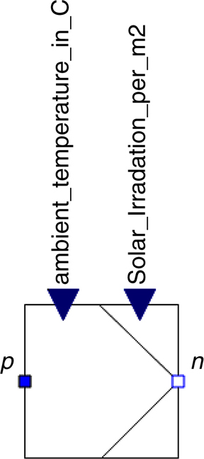
| Description | The photovoltaic module is a simplified model with two pins which converts solar irradiance and ambient temperature data into electrical active power depending on the surface area of the module. This power value is then used to compute the relation between voltage and current. When information on reactive power is not available, its value is set to zero as a default. The nominal operating conditions, such as ambient temperature, cell temperature, and radiation are parameters which may be chosen according to the specific PV panel in use. The efficiency is modeled to decrease at higher ambient temperatures than the nominal ambient temperature, depending on a temperature coefficient which depends on the type of PV panel. This model is not a component-based model like a diode PV model. Therefore, it is not useful for a detailed analysis of PV panel properties; it should rather be used to represent the behavior of a PV module as a source within an electric system (Fig. 4.10). |
| Parameters |
• Area (m2)
• Efficiency at nominal conditions
• Temperature coefficient for efficiency (°C−1)
• TNOCT Nominal operating cell temperature (°C)
• Tambient,NOCT NOCT Ambient temperature (°C)
• IrrNOCT NOCT irradiance on cell surface (W/m2)
• Q Reactive power (default = 0, W)
|
| Interfaces |
• Irr Solar irradiance input (W/m2)
• Tambient Ambient air temperature input (°C)
If a specific output is required, electrical quantities can be measured by connecting the corresponding sensor model. |
| Formulation | At first, the cell temperature Tcell is calculated from the ambient temperature input and the solar irradiance input, depending on the nominal operating conditions:
Now, the efficiency η is updated according to the difference between Tcell and TNOCT, weighted with the temperature coefficient for efficiency. Finally, according to Skoplaki and Palyvos (2009) the active power output is given as: P = Irr. area. η, which specifies the relationship between the dynamic phasor current and voltage across the two pins of the model with the equation:
|


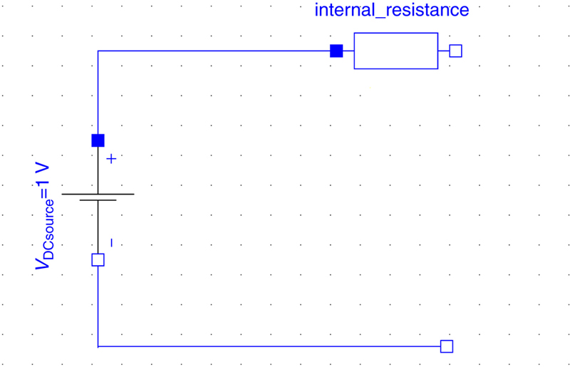
3.5.2.3. Simplified Battery Storage System
| Description | The battery storage system is a simple model of a generic battery. It can be charged or discharged up to a maximum capacity with a certain power and efficiency, while updating its state of charge. A charging or discharging logic can be connected to the battery via the charge/discharge status input. When information on the end-of-discharge or end-of-charge voltage are unknown, the default values can be used (Fig. 4.11). This model does not specify the battery technology and side effects which may occur due to the specific chemical processes some battery types use. |
| Parameters |
• SOCmax Storage capacity (Ah)
• SOC0 Initial state of charge (Ah)
• Rint Internal resistance of the battery (Ω)
• vnom Nominal voltage (V)
• vmin End-of-discharge voltage (default = 0.vnom)
• vmax End-of-charge voltage (default = 1.vnom)
• P Charging and discharging power (W)
• η Charging efficiency index (default = 1)
|
| Interfaces |
• Charge (0) or discharge (1) status input
|
| Formulation | The battery is modeled as a voltage source with an internal resistance, whose voltage level depends on the state of charge (Wagner, 2010). The battery storage is considered to operate in DC, a logic which translates between the dynamic phasor voltage and current in the rest of the system and their root mean square values was included within the battery model (Fig. 4.12). Assuming that the voltage source depends on the state of charge linearly for simplicity:
When the maximal storage capacity is reached, the voltage is limited by the end-of-charge voltage. In the first time step, SOC = SOC0. Through the power parameter, the DC current is computed from:
The state of charge is then updated through the equation:
while SOC ≤ SOCmax, and a = ±1 depending on whether the battery is charging or discharging. The current and voltage of the DC voltage source are converted back to AC as ideal sinusoidal signals with an adjustable default frequency of 50 Hz, where the amplitude is given by
|


3.5.2.4. Constant Power Load
| Description | Due to the difficulty of obtaining all physical load parameters, a simplified model representing the behavior of an electrical consumer with constant power was used. The relation between current and voltage necessary to characterize a two-pin component can be determined from the power values (Fig. 4.13). |
| Parameters |
• P active power (W)
• Q reactive power (var)
|
| Interfaces | If a specific output is required, electrical quantities can be measured by connecting the corresponding sensor model. |
| Formulation | The relation between the dynamic phasor current and voltage is given by the complex power:
|


3.5.2.5. EV Charger
| Description | The EV charger is a type of constant power load. It is an electrical consumer which, depending on the power level of the specific charging station, consumes the same amount of power during the time in which it is in use. By setting the status to “on,” the charging of an EV is simulated (Fig. 4.14). |
| Parameters | See constant power load. |
| Interfaces | Off (0) or on (1) status input. If a specific output is required, electrical quantities can be measured by connecting the corresponding sensor model. |
| Formulation | The formulation of the EV charger is the same as the constant power load except for the additional option of turning it off. This is achieved by setting the current equal to zero when the “off” state is given to the charger as input. |

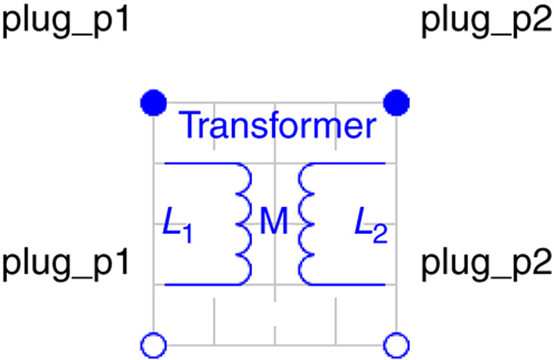
3.5.2.6. Transformer
| Description | For the transformer, an ideal model as well as a standard model is available for both single-phase and multiphase applications. The ideal transformer changes the voltage according to the turns ratio with an optional magnetization, whereas the standard transformer is modeled with two inductors and their mutual inductance (Fig. 4.15). Additionally, a prototype of a YY and YD transformer (YD5, YD11) have been modeled. |
| Parameters | Ideal transformer • n Turns ratio primary/secondary voltage
• Option for considering magnetization, default = false
• Lm
Magnetization inductance
Standard transformer: • L1 Self-inductance of winding1 (H)
• L2 Self-inductance of winding2 (H)
• M Mutual inductance (H)
|
| Interfaces | If a specific output is required, electrical quantities can be measured by connecting the corresponding sensor model. |
| Formulation | Ideal transformer The relation between the primary voltage v1 and the secondary voltage v2 is given by:
If the user chooses to consider the magnetization, the behavior is modified to include the magnetization current im (as a function of the primary current i1 and secondary current i2) and the magnetic flux ψm with respect to the primary side of the transformer:
Standard transformer The standard transformer also includes the primary and secondary inductance as well as their influence on each other. The equations then are:
Three-phase transformers The three-phase transformers are obtained by connecting single-phase transformers with a wye and/or delta connector. In case the ideal transformer is used, a resistor and inductor can be added in order to approximate the real behavior. The YY and YD transformers are models comprising the connection logic (wye or delta) and the transformer model (ideal or standard) as well as additional components if the ideal transformer model is used instead of the standard transformer. For example, the connection logic for a YD transformer is obtained by connecting components in series in the following order: • Wye connector
• Ideal transformer or standard transformer
• Internal resistance (only if the ideal transformer is used)
• Transformer stray inductance (only if the ideal transformer is used)
• Delta connector
|


3.5.2.7. Infinite Power Bus
| Description | The infinite power bus is used as a coupling point with the external electrical grid. It does not take the specific grid topology into account (Fig. 4.16). Therefore it is only suitable for studies of a system connected to the grid, but not to analyze the effects a system may have on the external grid. |
| Parameters |
• Amplitude (V)
• Frequency (Hz, default = 50 Hz)
• Phase
|
| Interfaces | If a specific output is required, electrical quantities of the infinite power bus can be measured by connecting the corresponding sensor model. |
| Formulation | The infinite power bus is modeled as an ideal sinusoidal voltage source according to the chosen parameters. |


3.5.2.8. Wind Turbine
| Description | The wind turbine model is a power curve model which, similarly to the solar PV generator, calculates an active power output depending on turbine specifications as well as the wind profile and air density (Fig. 4.17). Voltage and current information are then extracted from the power values. When information on reactive power is not available, it is set to null as a default. Since this is a function-based simplified model without mechanical information or the type of electrical generator, it is not useful for thorough studies of wind turbine properties, but should rather be used to represent a power source within an electrical system. |
| Parameters |
• cp power coefficient of the turbine, default = 0.593
• A swept area of the rotor (m2)
• ɛg generator efficiency, default = 1
• ɛb gearbox/bearings efficiency, default = 1
• Q reactive power, default = 0
|
| Interfaces |
• vwind wind velocity input (m/s)
• ρ air density input (kg/m3)
If a specific output is required, electrical quantities can be measured by connecting the corresponding sensor model. |
| Formulation | According to Ghosh and Prelas (2011), the active power curve of a wind turbine is described by the equation:
where
From the power output, the dynamic phasor voltage and current can be calculated with the equation:
|


4. Neighborhood Energy Optimization Algorithms
4.1. Mathematical Notations and Definitions
Table 4.3
Centralized Optimization algorithm—notations and definitions
| General |
N: prediction horizon
B: number of actors in the Neighborhood
|
| Generation | ||
| Combined Heat and Power (CHP) | Fossil Fuel Generators | Renewable generation |
PCHP,el,i : Electrical CHP output power PCHP,el,i_max : Max electrical CHP output power PCHP,el,i_min : Min electrical CHP output power PCHP,th,i : Thermal CHP output power ηCHP,el,i : Electrical CHP efficiency ηCHP,th,i : Thermal CHP efficiency sCHP,on,i ∈{0,1}:CHP ON/OFF state variable sCHP,up,i ∈{0,1}: Start command sCHP,down,i ∈{0,1}: Stop command ni ∈{1…8}: Minimum running time (time steps) |
Pboiler,i : Boiler output power Pboiler,i,min : Min boiler output power Pboiler,i,max : Max boiler output power ηboiler,th,i : Boiler efficiency sboiler,on,i ∈{0,1}: Boiler ON/OFF state variable PDiesel,i : Power produced by Diesel generator |
Prenew,i : Power produced by renewables |
| Storage |
Wth,i : Thermal energy stored in kWh Wth,i_max : Max thermal energy stored in kWh ηsto,th,i : Thermal storage efficiency Psto,in,i : Storage thermal charging power Psto,out,i : Storage thermal discharging power Psto,in,i_max : Max storage charging rate Psto,out,i_max : Max storage discharging rate Wel,i : Electrical energy stored Wel,i_max : Max electrical energy stored PC,i : Electrical storage charging power PD,i : Electrical storage discharging power PC,i_max : Max electrical storage charging power PD,i_max : Min electrical storage charging power ηC,i : Electrical storage charging efficiency |
| Consumption |
Lth,i : Thermal load of actor i Lel,i : Electrical load of actor i |

Table 4.4
Definitions—power purchases/sell, prices and costs
| Power purchases/sells | ||
| Outside grid (infinite power bus) | Neighborhood grid | Neighborhood energy exchange |
Pgb,i : Power purchased from the grid Pgs,i : Power sold to the grid |
Pnb,i : Power purchased from the Neighborhood Pns,i : Power sold to the Neighborhood |
Bi
: Profit of actor i when acting as an energy seller
Bj
: Savings of actor j when buying energy from the Neighborhood
Pn,i→j : Power exchanged from actor i to actor j (kW) Cn,i→j
: Price of the energy exchanged from actor i to actor j
xi→j : Ratio of power exchanged from actor i to j |
| Prices/costs | ||
| Fuel cost | Grid prices | Greenhouse emissions penalties |
Cgas,i : Cost of gas CDiesel,i : Cost of diesel |
Cgb,i : Cost of electrical energy imported from the grid Cgs,i : Reward for electrical energy grid exports Cnb,i : Cost of electrical energy imported from the Neighborhood Cns,i : Reward for electrical energy Neighborhood exports |
Ebs : The emissions of building b when the set of schedules S is selected |

4.1.1. Combined Heat and Power Mathematical Description
4.1.2. Boiler Mathematical Description
4.1.3. Thermal Storage Mathematical Description
4.1.4. Electrical Storage Mathematical Description
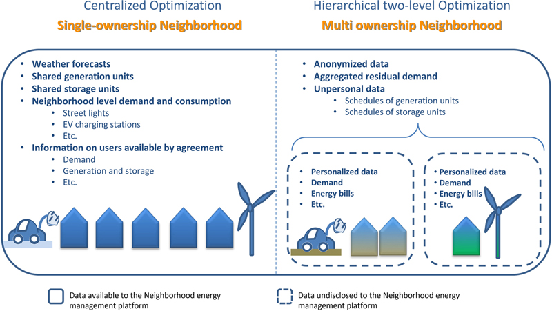
4.2. Centralized Optimization—Single Ownership Neighborhood


4.3. Hierarchical Two-Level Optimization


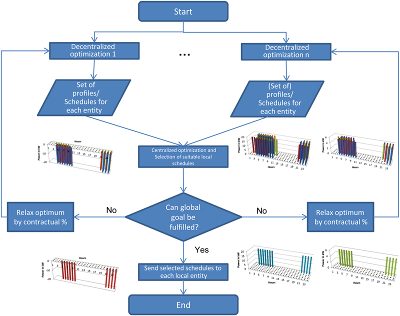

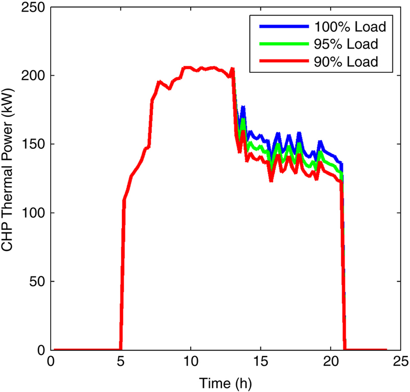
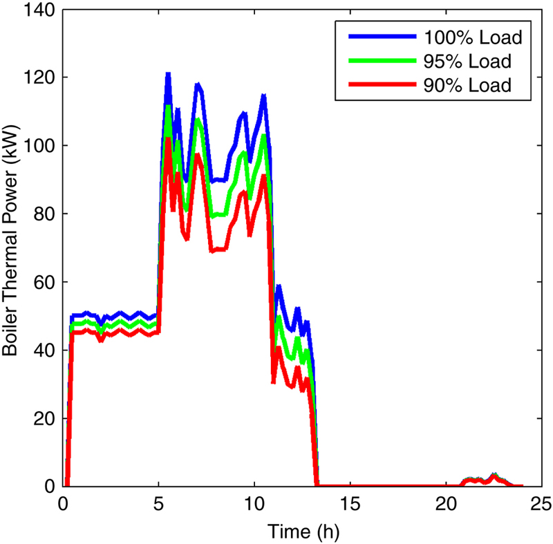
Table 4.5
Neighborhood-Level Optimization using Building Schedules Flexibility
