
2
Classical Optimization Techniques
2.1 Introduction
The classical methods of optimization are useful in finding the optimum solution of continuous and differentiable functions. These methods are analytical and make use of the techniques of differential calculus in locating the optimum points. Since some of the practical problems involve objective functions that are not continuous and/or differentiable, the classical optimization techniques have limited scope in practical applications. However, a study of the calculus methods of optimization forms a basis for developing most of the numerical techniques of optimization presented in subsequent chapters. In this chapter we present the necessary and sufficient conditions for locating the optimum solution of a single‐variable function, a multivariable function with no constraints, and a multivariable function with equality and inequality constraints.
2.2 Single‐Variable Optimization
A function of one variable f (x) is said to have a relative or local minimum at x = x* if f (x*) ≤ f (x* + h) for all sufficiently small positive and negative values of h. Similarly, a point x* is called a relative or local maximum if f (x*) ≥ f (x* + h) for all values of h sufficiently close to zero. A function f (x) is said to have a global or absolute minimum at x* if f (x*) ≤ f (x) for all x, and not just for all x close to x*, in the domain over which f (x) is defined. Similarly, a point x* will be a global maximum of f (x) if f (x*) ≥ f (x) for all x in the domain. Figure 2.1 shows the difference between the local and global optimum points.

Figure 2.1 Relative and global minima.
A single‐variable optimization problem is one in which the value of x = x* is to be found in the interval [a, b] such that x* minimizes f (x). The following two theorems provide the necessary and sufficient conditions for the relative minimum of a function of a single variable [1,2].
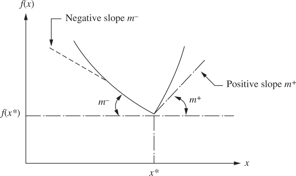
Figure 2.2 Derivative undefined at x*.
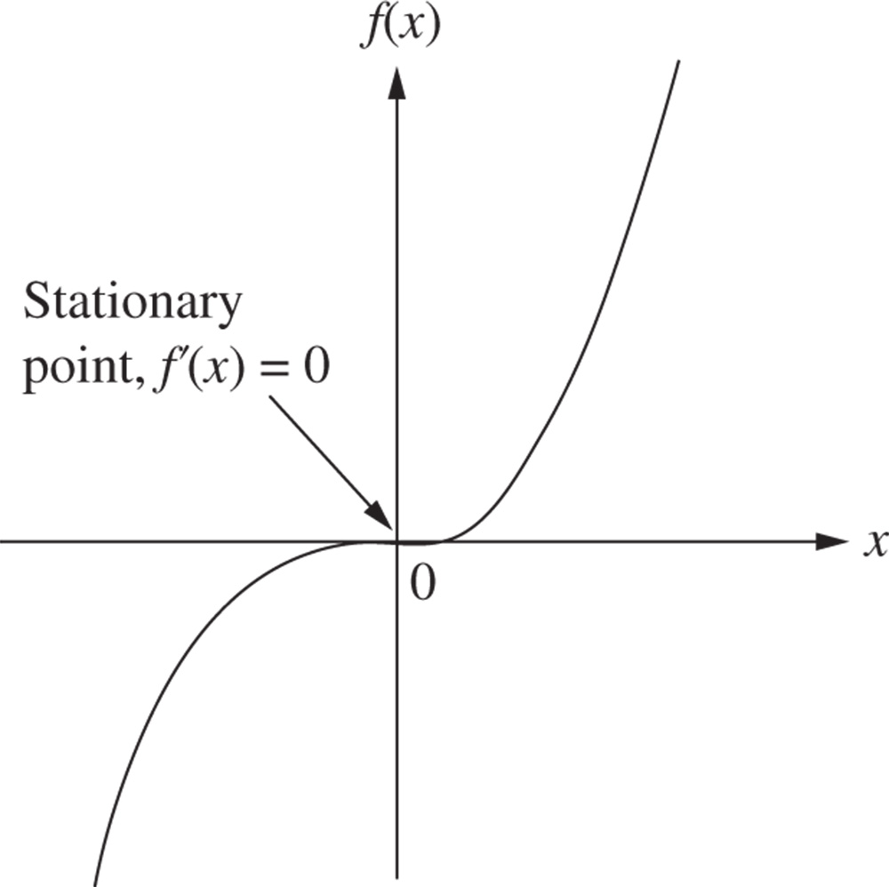
Figure 2.3 Stationary (inflection) point.
2.3 Multivariable Optimization with no Constraints
In this section we consider the necessary and sufficient conditions for the minimum or maximum of an unconstrained function of several variables [6,7]. Before seeing these conditions, we consider the Taylor's series expansion of a multivariable function.
2.3.1 Definition: rth Differential of f
If all partial derivatives of the function f through order r ≥ 1 exist and are continuous at a point X * , the polynomial

is called the rth differential of f at X*. Notice that there are r summations and one h i is associated with each summation in Eq. (2.6).
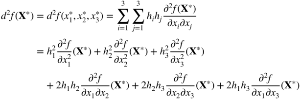
For example, when r = 2 and n = 3, we have
The Taylor's series expansion of a function f (X) about a point X* is given by

where the last term, called the remainder, is given by

where 0 < θ < 1 and h = X − X*.
2.3.2 Semidefinite Case
We now consider the problem of determining sufficient conditions for the case when the Hessian matrix of the given function is semidefinite. In the case of a function of a single variable, the problem of determining sufficient conditions for the case when the second derivative is zero was resolved quite easily. We simply investigated the higher‐order derivatives in the Taylor's series expansion. A similar procedure can be followed for functions of n variables. However, the algebra becomes quite involved, and hence we rarely investigate the stationary points for sufficiency in actual practice. The following theorem, analogous to Theorem 2.2, gives the sufficiency conditions for the extreme points of a function of several variables.
2.3.3 Saddle Point
In the case of a function of two variables, f (x, y), the Hessian matrix may be neither positive nor negative definite at a point (x*, y*) at which

In such a case, the point (x*, y*) is called a saddle point. The characteristic of a saddle point is that it corresponds to a relative minimum or maximum of f (x, y) with respect to one variable, say, x (the other variable being fixed at y = y*) and a relative maximum or minimum of f (x, y) with respect to the second variable y (the other variable being fixed at x*).
As an example, consider the function f (x, y) = x 2 − y 2. For this function,

These first derivatives are zero at x* = 0 and y* = 0. The Hessian matrix of f at (x*, y*) is given by
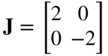
Since this matrix is neither positive definite nor negative definite, the point (x* = 0, y* = 0) is a saddle point. The function is shown graphically in Figure 2.5. It can be seen that f (x, y*) = f (x, 0) has a relative minimum and f (x*, y) = f (0, y) has a relative maximum at the saddle point (x*, y*). Saddle points may exist for functions of more than two variables also. The characteristic of the saddle point stated above still holds provided that x and y are interpreted as vectors in multidimensional cases.

Figure 2.5 Saddle point of the function f (x, y) = x 2 − y 2.
2.4 Multivariable Optimization with Equality Constraints
In this section we consider the optimization of continuous functions subjected to equality constraints:

where

Here m is less than or equal to n; otherwise (if m > n), the problem becomes overdefined and, in general, there will be no solution. There are several methods available for the solution of this problem. The methods of direct substitution, constrained variation, and Lagrange multipliers are discussed in the following sections [8–10].
2.4.1 Solution by Direct Substitution
For a problem with n variables and m equality constraints, it is theoretically possible to solve simultaneously the m equality constraints and express any set of m variables in terms of the remaining n − m variables. When these expressions are substituted into the original objective function, there results a new objective function involving only n − m variables. The new objective function is not subjected to any constraint, and hence its optimum can be found by using the unconstrained optimization techniques discussed in Section 2.3.
This method of direct substitution, although it appears to be simple in theory, is not convenient from a practical point of view. The reason for this is that the constraint equations will be nonlinear for most of practical problems, and often it becomes impossible to solve them and express any m variables in terms of the remaining n − m variables. However, the method of direct substitution might prove to be very simple and direct for solving simpler problems, as shown by the following example.
2.4.2 Solution by the Method of Constrained Variation
The basic idea used in the method of constrained variation is to find a closed‐form expression for the first‐order differential of f (df) at all points at which the constraints g j (X) = 0, j = 1, 2, …, m, are satisfied. The desired optimum points are then obtained by setting the differential df equal to zero. Before presenting the general method, we indicate its salient features through the following simple problem with n = 2 and m = 1:
subject to
A necessary condition for f to have a minimum at some point ![]() is that the total derivative of f (x
1, x
2) with respect to x
1 must be zero at
is that the total derivative of f (x
1, x
2) with respect to x
1 must be zero at ![]() . By setting the total differential of f (x
1, x
2) equal to zero, we obtain
. By setting the total differential of f (x
1, x
2) equal to zero, we obtain

Since ![]() at the minimum point, any variations dx
1 and dx
2 taken about the point
at the minimum point, any variations dx
1 and dx
2 taken about the point ![]() are called admissible variations provided that the new point lies on the constraint:
are called admissible variations provided that the new point lies on the constraint:
The Taylor's series expansion of the function in Eq. (2.20) about the point ![]() gives
gives
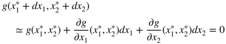
where dx
1 and dx
2 are assumed to be small. Since ![]() , Eq. (2.21) reduces to
, Eq. (2.21) reduces to

Thus Eq. (2.22) has to be satisfied by all admissible variations. This is illustrated in Figure 2.6, where PQ indicates the curve at each point of which Eq. (2.18) is satisfied. If A is taken as the base point ![]() , the variations in x
1 and x
2 leading to points B and C are called admissible variations. On the other hand, the variations in x
1 and x
2 representing point D are not admissible since point D does not lie on the constraint curve, g (x
1, x
2) = 0. Thus any set of variations (dx
1, dx
2) that does not satisfy Eq. (2.22) leads to points such as D, which do not satisfy constraint Eq. (2.18).
, the variations in x
1 and x
2 leading to points B and C are called admissible variations. On the other hand, the variations in x
1 and x
2 representing point D are not admissible since point D does not lie on the constraint curve, g (x
1, x
2) = 0. Thus any set of variations (dx
1, dx
2) that does not satisfy Eq. (2.22) leads to points such as D, which do not satisfy constraint Eq. (2.18).

Figure 2.6 Variations about A.
Assuming that ∂g/∂x 2 ≠ 0, Eq. (2.22) can be rewritten as
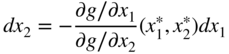
This relation indicates that once the variation in x 1(dx 1) is chosen arbitrarily, the variation in x 2 (dx 2) is decided automatically in order to have dx 1 and dx 2 as a set of admissible variations. By substituting Eq. (2.23) in Eq. (2.19), we obtain

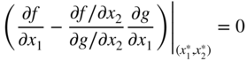
The expression on the left‐hand side is called the constrained variation of f. Note that Eq. (2.24) has to be satisfied for all values of dx 1. Since dx 1 can be chosen arbitrarily, Eq. (2.24) leads to

Equation (2.25) represents a necessary condition in order to have ![]() as an extreme point (minimum or maximum).
as an extreme point (minimum or maximum).
Necessary Conditions for a General Problem
The procedure indicated above can be generalized to the case of a problem in n variables with m constraints. In this case, each constraint equation g j (X) = 0, j = 1, 2, …, m, gives rise to a linear equation in the variations dx i , i = 1, 2, …, n. Thus, there will be in all m linear equations in n variations. Hence, any m variations can be expressed in terms of the remaining n − m variations. These expressions can be used to express the differential of the objective function, df, in terms of the n − m independent variations. By letting the coefficients of the independent variations vanish in the equation df = 0, one obtains the necessary conditions for the constrained optimum of the given function. These conditions can be expressed as [7]

where k = m + 1, m + 2, …, n. It is to be noted that the variations of the first m variables (dx 1, dx 2, …, dx m ) have been expressed in terms of the variations of the remaining n − m variables (dx m+1, dx m+2, …, dx n ) in deriving Eq. (2.26). This implies that the following relation is satisfied:

The n − m equations given by Eq. (2.26) represent the necessary conditions for the extremum of f (X) under the m equality constraints, g j (X) = 0, j = 1, 2, …, m.
Sufficiency Conditions for a General Problem
By eliminating the first m variables, using the m equality constraints (this is possible, at least in theory), the objective function f can be made to depend only on the remaining variables, x m+1, x m+2, …, x n . Then the Taylor's series expansion of f, in terms of these variables, about the extreme point X* gives

where (∂f/∂x i ) g is used to denote the partial derivative of f with respect to x i (holding all the other variables x m+1, x m+2, …, x i−1, x i+1, x i+2, …, x n constant) when x 1, x 2, …, x m are allowed to change so that the constraints g j (X* + d X) = 0, j = 1, 2, …, m, are satisfied; the second derivative, (∂ 2 f/∂x i ∂x j ) g , is used to denote a similar meaning.
As an example, consider the problem of minimizing
subject to the only constraint
Since n = 3 and m = 1 in this problem, one can think of any of the m variables, say x 1, to be dependent and the remaining n − m variables, namely x 2 and x 3, to be independent. Here the constrained partial derivative (∂f/∂x 2) g , for example, means the rate of change of f with respect to x 2 (holding the other independent variable x 3 constant) and at the same time allowing x 1 to change about X* so as to satisfy the constraint g 1 (X) = 0. In the present case, this means that dx 1 has to be chosen to satisfy the relation

that is,
since g 1 (X*) = 0 at the optimum point and dx 3 = 0 (x 3 is held constant).
Notice that (∂f/∂x i ) g has to be zero for i = m + 1, m + 2, …, n since the dx i appearing in Eq. (2.28) are all independent. Thus, the necessary conditions for the existence of constrained optimum at X* can also be expressed as

Of course, with little manipulation, one can show that Eqs. (2.29) are nothing but Eq. (2.26). Further, as in the case of optimization of a multivariable function with no constraints, one can see that a sufficient condition for X* to be a constrained relative minimum (maximum) is that the quadratic form Q defined by

is positive (negative) for all nonvanishing variations dx i . As in Theorem 2.4, the matrix

has to be positive (negative) definite to have Q positive (negative) for all choices of dx i . It is evident that computation of the constrained derivatives (∂ 2 f/∂x i ∂x j ) g is a difficult task and may be prohibitive for problems with more than three constraints. Thus, the method of constrained variation, although it appears to be simple in theory, is very difficult to apply since the necessary conditions themselves involve evaluation of determinants of order m + 1. This is the reason that the method of Lagrange multipliers, discussed in the following section, is more commonly used to solve a multivariable optimization problem with equality constraints.
2.4.3 Solution By the Method of Lagrange Multipliers
The basic features of the Lagrange multiplier method is given initially for a simple problem of two variables with one constraint. The extension of the method to a general problem of n variables with m constraints is given later.
Problem with Two Variables and One Constraint
Consider the problem
subject to
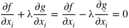
For this problem, the necessary condition for the existence of an extreme point at X = X* was found in Section 2.4.2 to be
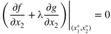
By defining a quantity λ, called the Lagrange multiplier, as

Equation (2.32) can be expressed as

and Eq. (2.33) can be written as
In addition, the constraint equation has to be satisfied at the extreme point, that is,
Thus Eqs. (2.34)–(2.36) represent the necessary conditions for the point ![]() to be an extreme point.
to be an extreme point.
Notice that the partial derivative ![]() has to be nonzero to be able to define λ by Eq. (2.33). This is because the variation dx
2 was expressed in terms of dx
1 in the derivation of Eq. (2.32) (see Eq. (2.23)). On the other hand, if we choose to express dx
1 in terms of dx
2, we would have obtained the requirement that
has to be nonzero to be able to define λ by Eq. (2.33). This is because the variation dx
2 was expressed in terms of dx
1 in the derivation of Eq. (2.32) (see Eq. (2.23)). On the other hand, if we choose to express dx
1 in terms of dx
2, we would have obtained the requirement that ![]() be nonzero to define λ. Thus, the derivation of the necessary conditions by the method of Lagrange multipliers requires that at least one of the partial derivatives of g (x
1, x
2) be nonzero at an extreme point.
be nonzero to define λ. Thus, the derivation of the necessary conditions by the method of Lagrange multipliers requires that at least one of the partial derivatives of g (x
1, x
2) be nonzero at an extreme point.
The necessary conditions given by Eqs. (2.34)–(2.36) are more commonly generated by constructing a function L, known as the Lagrange function, as
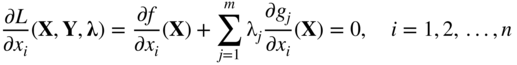
By treating L as a function of the three variables x 1, x 2, and λ, the necessary conditions for its extremum are given by
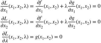
Equations (2.38) can be seen to be same as Eqs. (2.34)–(2.36). The sufficiency conditions are given later.
Necessary Conditions for a General Problem
The equations derived above can be extended to the case of a general problem with n variables and m equality constraints:
subject to
The Lagrange function, L, in this case is defined by introducing one Lagrange multiplier λ j for each constraint g j (X) as

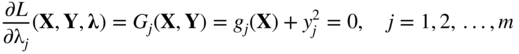
By treating L as a function of the n + m unknowns, x 1, x 2, …, x n , λ1, λ2, …, λ m , the necessary conditions for the extremum of L, which also correspond to the solution of the original problem stated in Eq. (2.39), are given by


Equations (2.41) and (2.42) represent n + m equations in terms of the n + m unknowns, x i and λ j . The solution of Eqs. (2.41) and (2.42) gives
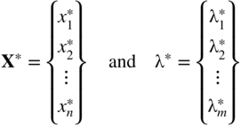
The vector X* corresponds to the relative constrained minimum of f (X) (sufficient conditions are to be verified) while the vector λ* provides the sensitivity information, as discussed in the next subsection.
Sufficiency Conditions for a General Problem
A sufficient condition for f (X) to have a constrained relative minimum at X* is given by the following theorem.
Interpretation of the Lagrange Multipliers
To find the physical meaning of the Lagrange multipliers, consider the following optimization problem involving only a single equality constraint:
subject to
where b is a constant. The necessary conditions to be satisfied for the solution of the problem are

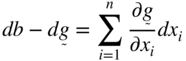
Let the solution of Eqs. (2.49) and (2.50) be given by X*, λ*, and f* = f (X*). Suppose that we want to find the effect of a small relaxation or tightening of the constraint on the optimum value of the objective function (i.e. we want to find the effect of a small change in b on f*). For this we differentiate Eq. (2.48) to obtain
or
Equation (2.49) can be rewritten as
or

Substituting Eq. (2.53) into Eq. (2.51), we obtain

since

Equation (2.54) gives

or
Thus λ* denotes the sensitivity (or rate of change) of f with respect to b or the marginal or incremental change in f* with respect to b at x*. In other words, λ* indicates how tightly the constraint is binding at the optimum point. Depending on the value of λ* (positive, negative, or zero), the following physical meaning can be attributed to λ*:
- λ* > 0. In this case, a unit decrease in b is positively valued since one gets a smaller minimum value of the objective function f. In fact, the decrease in f* will be exactly equal to λ* since df = λ* (−1) = −λ* < 0. Hence λ* may be interpreted as the marginal gain (further reduction) in f* due to the tightening of the constraint. On the other hand, if b is increased by 1 unit, f will also increase to a new optimum level, with the amount of increase in f* being determined by the magnitude of λ* since df = λ*(+1) > 0. In this case, λ* may be thought of as the marginal cost (increase) in f* due to the relaxation of the constraint.
- λ* < 0. Here a unit increase in b is positively valued. This means that it decreases the optimum value of f. In this case the marginal gain (reduction) in f* due to a relaxation of the constraint by 1 unit is determined by the value of λ* as df* = λ*(+1) < 0. If b is decreased by 1 unit, the marginal cost (increase) in f* by the tightening of the constraint is df* = λ*(−1) > 0 since, in this case, the minimum value of the objective function increases.
- λ* = 0. In this case, any incremental change in b has absolutely no effect on the optimum value of f and hence the constraint will not be binding. This means that the optimization of f subject to g = 0 leads to the same optimum point X* as with the unconstrained optimization of f
In economics and operations research, Lagrange multipliers are known as shadow prices of the constraints since they indicate the changes in optimal value of the objective function per unit change in the right‐hand side of the equality constraints.
2.5 Multivariable Optimization with Inequality Constraints
This section is concerned with the solution of the following problem:
subject to
The inequality constraints in Eq. (2.58) can be transformed to equality constraints by adding nonnegative slack variables, ![]() , as
, as
where the values of the slack variables are yet unknown. The problem now becomes
subject to
where Y = {y 1, y 2, …, y m }T is the vector of slack variables.
This problem can be solved conveniently by the method of Lagrange multipliers. For this, we construct the Lagrange function L as

where λ = {λ1, λ2, …, λ m }T is the vector of Lagrange multipliers. The stationary points of the Lagrange function can be found by solving the following equations (necessary conditions):

It can be seen that Eqs. (2.62)–(2.64) represent (n + 2m) equations in the (n + 2m) unknowns, X, λ, and Y. The solution of Eqs. (2.62)–(2.64) thus gives the optimum solution vector, X*; the Lagrange multiplier vector, λ*; and the slack variable vector, Y*.
Equations (2.63) ensure that the constraints g j (X) ≤ 0, j = 1, 2, …, m, are satisfied, while Eq. (2.64) imply that either λ j = 0 or y j = 0. If λ j = 0, it means that the jth constraint is inactive1 and hence can be ignored. On the other hand, if y j = 0, it means that the constraint is active (g j = 0) at the optimum point. Consider the division of the constraints into two subsets, J 1 and J 2, where J 1 + J 2 represent the total set of constraints. Let the set J 1 indicate the indices of those constraints that are active at the optimum point and J 2 include the indices of all the inactive constraints.
Thus, for j ∈ J 1,2 y j = 0 (constraints are active), for j ∈ J 2, λ j = 0 (constraints are inactive), and Eq. (2.62) can be simplified as
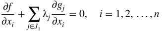
Similarly, Eq. (2.63) can be written as
Equations (2.65)–(2.67) represent n + p + (m − p) = n + m equations in the n + m unknowns x i (i = 1, 2, …, n), λ j (j ∈ J 1), and y j (j ∈ J 2), where p denotes the number of active constraints.
Assuming that the first p constraints are active, Eq. (2.65) can be expressed as

These equations can be written collectively as
where ∇f and ∇g j are the gradients of the objective function and the jth constraint, respectively:

Equation (2.69) indicates that the negative of the gradient of the objective function can be expressed as a linear combination of the gradients of the active constraints at the optimum point.
Further, we can show that in the case of a minimization problem, the λ j values (j ∈ J 1) have to be positive. For simplicity of illustration, suppose that only two constraints are active (p = 2) at the optimum point. Then Eq. (2.69) reduces to
Let S be a feasible direction3 at the optimum point. By premultiplying both sides of Eq. (2.70) by S T , we obtain
where the superscript T denotes the transpose. Since S is a feasible direction, it should satisfy the relations


Figure 2.8 Feasible direction S.
Thus, if λ1 > 0 and λ2 > 0, the quantity S T ∇ f can be seen always to be positive. As ∇f indicates the gradient direction, along which the value of the function increases at the maximum rate,4 S T ∇ f represents the component of the increment of f along the direction S. If S T ∇ f > 0, the function value increases as we move along the direction S. Hence, if λ1 and λ2 are positive, we will not be able to find any direction in the feasible domain along which the function value can be decreased further. Since the point at which Eq. (2.72) is valid is assumed to be optimum, λ1 and λ2 have to be positive. This reasoning can be extended to cases where there are more than two constraints active. By proceeding in a similar manner, one can show that the λ j values have to be negative for a maximization problem.
2.5.1 Kuhn–Tucker Conditions
As shown above, the conditions to be satisfied at a constrained minimum point, X*, of the problem stated in Eq. (2.58) can be expressed as

These are called Kuhn–Tucker conditions after the mathematicians who derived them as the necessary conditions to be satisfied at a relative minimum of f (X) [11]. These conditions are, in general, not sufficient to ensure a relative minimum. However, there is a class of problems, called convex programming problems,5 for which the Kuhn–Tucker conditions are necessary and sufficient for a global minimum.
If the set of active constraints is not known, the Kuhn–Tucker conditions can be stated as follows:

Note6 that if the problem is one of maximization or if the constraints are of the type g j ≥ 0, the λ j have to be nonpositive in Eq. (2.75). On the other hand, if the problem is one of maximization with constraints in the form g j ≥ 0, the λ j have to be nonnegative in Eq. (2.75).
2.5.2 Constraint Qualification
When the optimization problem is stated as
subject to
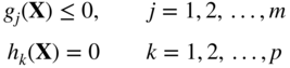
the Kuhn–Tucker conditions become

where λ j and β k denote the Lagrange multipliers associated with the constraints g j ≤ 0 and h k = 0, respectively. Although we found qualitatively that the Kuhn–Tucker conditions represent the necessary conditions of optimality, the following theorem gives the precise conditions of optimality.
2.6 Convex Programming Problem
The optimization problem stated in Eq. (2.58) is called a convex programming problem if the objective function f (X) and the constraint functions g j (X) are convex. The definition and properties of a convex function are given in Appendix A. Suppose that f (X) and g j (X), j = 1, 2, …, m, are convex functions. The Lagrange function of Eq. (2.61) can be written as
If λ j ≥ 0, then λ j g j (X) is convex, and since λ j y j = 0 from Eq. (2.64), L (X, Y, λ) will be a convex function. As shown earlier, a necessary condition for f (X) to be a relative minimum at X* is that L (X, Y, λ) have a stationary point at X*. However, if L (X, Y, λ) is a convex function, its derivative vanishes only at one point, which must be an absolute minimum of the function f (X). Thus, the Kuhn–Tucker conditions are both necessary and sufficient for an absolute minimum of f (X) at X*.
Notes:
- If the given optimization problem is known to be a convex programming problem, there will be no relative minima or saddle points, and hence the extreme point found by applying the Kuhn–Tucker conditions is guaranteed to be an absolute minimum of f (X). However, it is often very difficult to ascertain whether the objective and constraint functions involved in a practical engineering problem are convex.
- The derivation of the Kuhn–Tucker conditions was based on the development given for equality constraints in Section 2.4. One of the requirements for these conditions was that at least one of the Jacobians composed of the m constraints and m of the n + m variables (x 1, x 2, …, x n ; y 1, y 2, …, y m ) be nonzero. This requirement is implied in the derivation of the Kuhn–Tucker conditions.
References and Bibliography
- 1 Hancock, H. (1960). Theory of Maxima and Minima. Dover, NY: Dover Publications.
- 2 Levenson, M.E. (1967). Maxima and Minima. New York: Macmillan.
- 3 Thomas, G.B. Jr. (1967). Calculus and Analytic Geometry. Reading, MA: Addison‐Wesley.
- 4 Richmond, A.E. (1972). Calculus for Electronics. New York: McGraw‐Hill.
- 5 Howell, J.R. and Buckius, R.O. (1992). Fundamentals of Engineering Thermodynamics, 2e. New York: McGraw‐Hill.
- 6 Kolman, B. and Trench, W.F. (1971). Elementary Multivariable Calculus. New York: Academic Press.
- 7 Beveridge, G.S.G. and Schechter, R.S. (1970). Optimization: Theory and Practice. New York: McGraw‐Hill.
- 8 Gue, R. and Thomas, M.E. (1968). Mathematical Methods of Operations Research. New York: Macmillan.
- 9 Ayres, F. Jr. (1962). Theory and Problems of Matrices, Schaum's Outline Series. New York: Schaum.
- 10 Panik, M.J. (1976). Classical Optimization: Foundations and Extensions. North‐Holland, Amsterdam.
- 11 Kuhn, H.W. and Tucker, A. (1951). Nonlinear programming. In: Proceedings of the 2nd Berkeley Symposium on Mathematical Statistics and Probability. Berkeley: University of California Press.
- 12 Bazaraa, M.S. and Shetty, C.M. (1979). Nonlinear Programming: Theory and Algorithms. New York: Wiley.
- 13 Simmons, D.M. (1975). Nonlinear Programming for Operations Research. Engle‐wood Cliffs, NJ: Prentice Hall.
Review Questions
- 1 1 State the necessary and sufficient conditions for the minimum of a function f (x).
- 2 2 Under what circumstances can the condition df (x)/dx = 0 not be used to find the minimum of the function f (x)?
- 3 3 Define the rth differential, d r f (X), of a multivariable function f (X).
- 4 4 Write the Taylor's series expansion of a function f (X).
- 5 5 State the necessary and sufficient conditions for the maximum of a multivariable function f (X).
- 6 6 What is a quadratic form?
- 7 7 How do you test the positive, negative, or indefiniteness of a square matrix [A]?
- 8 8 Define a saddle point and indicate its significance.
- 9 9 State the various methods available for solving a multivariable optimization problem with equality constraints.
- 10 10 State the principle behind the method of constrained variation.
- 11 11 What is the Lagrange multiplier method?
- 12 12 What is the significance of Lagrange multipliers?
- 13 13 Convert an inequality constrained problem into an equivalent unconstrained problem.
- 14 14 State the Kuhn–Tucker conditions.
- 15 15 What is an active constraint?
- 16 16 Define a usable feasible direction.
- 17 17 What is a convex programming problem? What is its significance?
- 18 Answer whether each of the following quadratic forms is positive definite, negative definite, or neither:
- (18) (18)

- (18) (18) f = 4x 1 x 2
- (18) (18)

- (18) (18)
- (18) (18)

- (18) (18)
- 19 State whether each of the following functions is convex, concave, or neither:
- (19) (19) f = − 2x 2 + 8x + 4
- (19) (19) f = x 2 + 10x + 1
- (19) (19)
- (19) (19)

- (19) (19) f = e −x , x > 0
- (19) (19)

- (19) (19) f = x 1 x 2
- (19) (19) f = (x 1 − 1)2 + 10(x 2 − 2)2
- 20 20 Match the following equations and their characteristics:
(a) f = 4x 1 − 3x 2 + 2 Relative maximum at (1, 2) (b) f = (2x 1 − 2)2 + (x 2 − 2)2 Saddle point at origin (c) f = − (x 1 − 1)2 − (x 2 − 2)2 No minimum (d) f = x 1 x 2 Inflection point at origin (e) f = x 3 Relative minimum at (1, 2)
Problems
- 2.1
A dc generator has an internal resistance R ohms and develops an open‐circuit voltage of V volts (Figure 2.10). Find the value of the load resistance r for which the power delivered by the generator will be a maximum.

Figure 2.10 Electric generator with load. - 2.2
Find the maxima and minima, if any, of the function

- 2.3
Find the maxima and minima, if any, of the function
- 2.4 The efficiency of a screw jack is given by

where α is the lead angle and ϕ is a constant. Prove that the efficiency of the screw jack will be maximum when α = 45° − ϕ/2 with η max = (1 − sin ϕ)/(1 + sin ϕ).
- 2.5
Find the minimum of the function

- 2.6 Find the angular orientation of a cannon to maximize the range of the projectile.
- 2.7
In a submarine telegraph cable the speed of signaling varies as x
2 log (1/x), where x is the ratio of the radius of the core to that of the covering. Show that the greatest speed is attained when this ratio is
 .
. - 2.8 The horsepower generated by a Pelton wheel is proportional to u (V − u), where u is the velocity of the wheel, which is variable, and V is the velocity of the jet, which is fixed. Show that the efficiency of the Pelton wheel will be maximum when u = V/2.
- 2.9 A pipe of length l and diameter D has at one end a nozzle of diameter d through which water is discharged from a reservoir. The level of water in the reservoir is maintained at a constant value h above the center of nozzle. Find the diameter of the nozzle so that the kinetic energy of the jet is a maximum. The kinetic energy of the jet can be expressed as

where ρ is the density of water, f the friction coefficient and g the gravitational constant.
- 2.10 An electric light is placed directly over the center of a circular plot of lawn 100 m in diameter. Assuming that the intensity of light varies directly as the sine of the angle at which it strikes an illuminated surface, and inversely as the square of its distance from the surface, how high should the light be hung in order that the intensity may be as great as possible at the circumference of the plot?
- 2.11 If a crank is at an angle θ from dead center with θ = ωt, where ω is the angular velocity and t is time, the distance of the piston from the end of its stroke (x) is given by

where r is the length of the crank and l is the length of the connecting rod. For r = 1 and l = 5, find (a) the angular position of the crank at which the piston moves with maximum velocity, and (b) the distance of the piston from the end of its stroke at that instant.
Determine whether each of the matrices in Problems 2.12–2.14 is positive definite, negative definite, or indefinite by finding its eigenvalues.
- 2.12

- 2.13
- 2.14

Determine whether each of the matrices in Problems 2.15–2.17 is positive definite, negative definite, or indefinite by evaluating the signs of its submatrices.
- 2.15

- 2.16
- 2.17

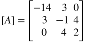
- 2.18 Express the function

in matrix form as
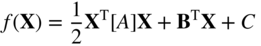
and determine whether the matrix [A] is positive definite, negative definite, or indefinite.
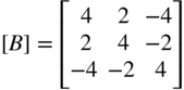
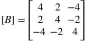
- 2.19
Determine whether the following matrix is positive or negative definite:

- 2.20
Determine whether the following matrix is positive definite:
- 2.21 The potential energy of the two‐bar truss shown in Figure 2.11 is given by

where E is Young's modulus, A the cross‐sectional area of each member, l the span of the truss, s the length of each member, h the height of the truss, P the applied load, θ the angle at which the load is applied, and x 1 and x 2 are, respectively, the horizontal and vertical displacements of the free node. Find the values of x 1 and x 2 that minimize the potential energy when E = 207 × 109 Pa, A = 10−5 m2, l = 1.5 m, h = 4.0 m, P = 104 N, and θ = 30°
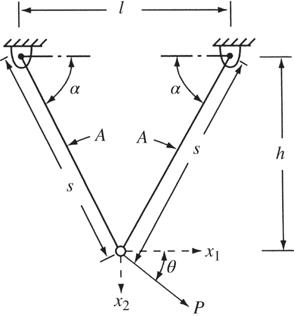
Figure 2.11 Two‐bar truss.
- 2.22 The profit per acre of a farm is given by
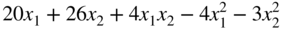
where x 1 and x 2 denote, respectively, the labor cost and the fertilizer cost. Find the values of x 1 and x 2 to maximize the profit.
- 2.23 The temperatures measured at various points inside a heated wall are as follows:
Distance from the heated surface as a percentage of wall thickness, d 0 25 50 75 100 Temperature, t(°C) 380 200 100 20 0 It is decided to approximate this table by a linear equation (graph) of the form t = a + bd, where a and b are constants. Find the values of the constants a and b that minimize the sum of the squares of all differences between the graph values and the tabulated values.
- 2.24 Find the second‐order Taylor's series approximation of the function
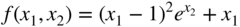
at the points (a) (0,0) and (b) (1,1).
- 2.25 Find the third‐order Taylor's series approximation of the function

at point (1, 0, −2).
- 2.26 The volume of sales (f) of a product is found to be a function of the number of newspaper advertisements (x) and the number of minutes of television time (y) as

Each newspaper advertisement or each minute on television costs $1000. How should the firm allocate $48 000 between the two advertising media for maximizing its sales?
- 2.27
Find the value of x* at which the following function attains its maximum:

- 2.28 (a) (b) (c) (d) It is possible to establish the nature of stationary points of an objective function based on its quadratic approximation. For this, consider the quadratic approximation of a two‐variable function as

where

If the eigenvalues of the Hessian matrix, [c], are denoted as β 1 and β 2, identify the nature of the contours of the objective function and the type of stationary point in each of the following situations.
- (a) β 1 = β 2; both positive
- (b) β 1 > β 2; both positive
- (c) |β 1| = |β 2|; β 1 and β 2 have opposite signs
- (d) β 1 > 0, β 2 = 0
Plot the contours of each of the following functions and identify the nature of its stationary point.
- 2.29 f = 2 − x 2 − y 2 + 4xy
- 2.30 f = 2 + x 2 − y 2
- 2.31 f = xy
- 2.32 f = x 3 − 3xy 2
- 2.33 Find the admissible and constrained variations at the point X = {0, 4}T for the following problem:

subject to

- 2.34 Find the diameter of an open cylindrical can that will have the maximum volume for a given surface area, S.
- 2.35 A rectangular beam is to be cut from a circular log of radius r. Find the cross‐sectional dimensions of the beam to (a) maximize the cross‐sectional area of the beam, and (b) maximize the perimeter of the beam section.
- 2.36 Find the dimensions of a straight beam of circular cross section that can be cut from a conical log of height h and base radius r to maximize the volume of the beam.
- 2.37 The deflection of a rectangular beam is inversely proportional to the width and the cube of depth. Find the cross‐sectional dimensions of a beam, which corresponds to minimum deflection, that can be cut from a cylindrical log of radius r.
- 2.38
A rectangular box of height a and width b is placed adjacent to a wall (Figure 2.12). Find the length of the shortest ladder that can be made to lean against the wall.
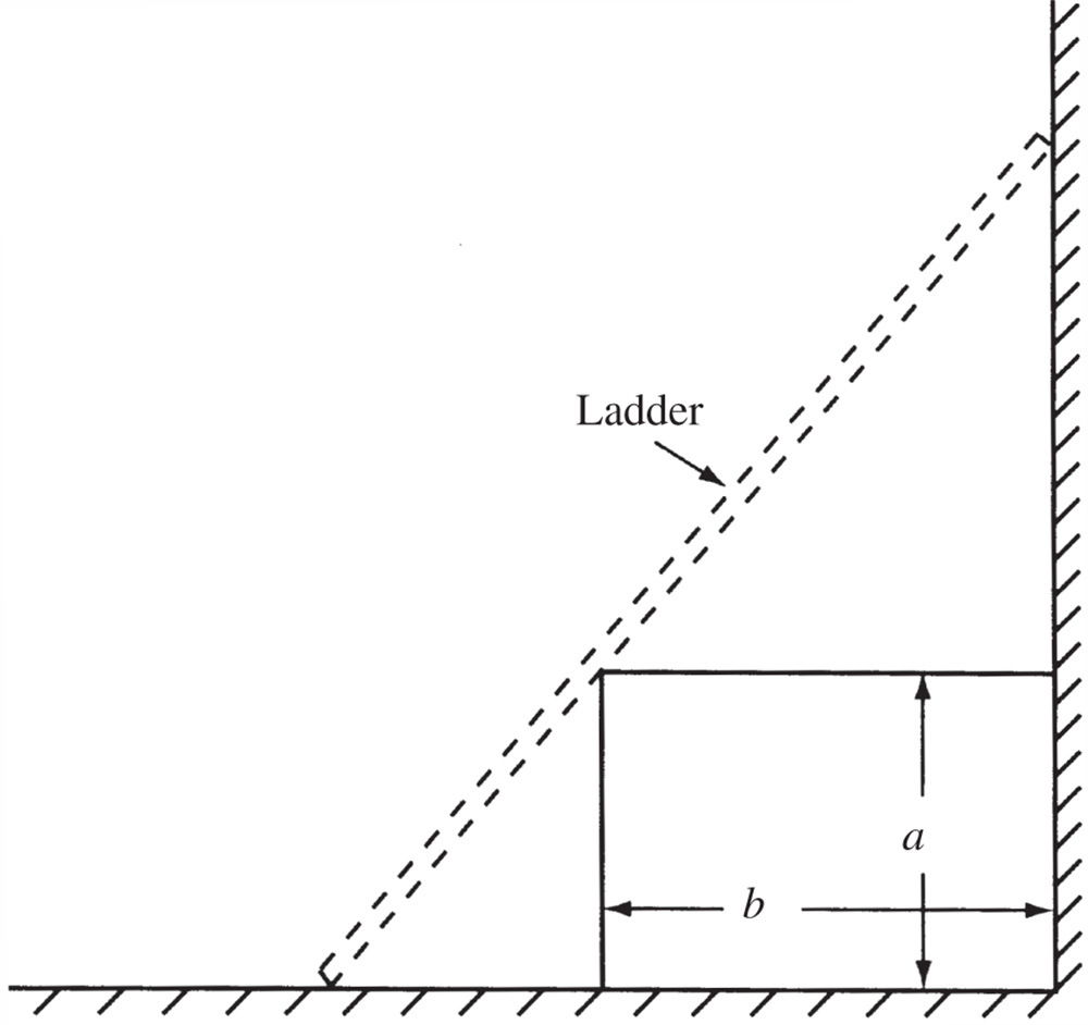
Figure 2.12 Ladder against a wall. - 2.39 Show that the right circular cylinder of given surface (including the ends) and maximum volume is such that its height is equal to the diameter of the base.
- 2.40 Find the dimensions of a closed cylindrical soft drink can that can hold soft drink of volume V for which the surface area (including the top and bottom) is a minimum.
- 2.41 An open rectangular box is to be manufactured from a given amount of sheet metal (area S). Find the dimensions of the box to maximize the volume.
- 2.42 Find the dimensions of an open rectangular box of volume V for which the amount of material required for manufacture (surface area) is a minimum.
- 2.43 A rectangular sheet of metal with sides a and b has four equal square portions (of side d) removed at the corners, and the sides are then turned up in order to form an open rectangular box. Find the depth of the box that maximizes the volume.
- 2.44 Show that the cone of the greatest volume that can be inscribed in a given sphere has an altitude equal to two‐thirds of the diameter of the sphere. Also prove that the curved surface of the cone is a maximum for the same value of the altitude.
- 2.45 Prove Theorem 2.6.
- 2.46 A log of length l is in the form of a frustum of a cone whose ends have radii a and b(a > b). It is required to cut from it a beam of uniform square section. Prove that the beam of greatest volume that can be cut has a length of al/[3(a − b)].
- 2.47 It has been decided to leave a margin of 30 mm at the top and 20 mm each at the left side, right side, and the bottom on the printed page of a book. If the area of the page is specified as 5 × 104 mm2, determine the dimensions of a page that provide the largest printed area.
- 2.48
subject to

by (a) direct substitution, (b) constrained variation, and (c) Lagrange multiplier method.
- 2.49

subject to
by (a) direct substitution, (b) constrained variation, and (c) Lagrange multiplier method.
- 2.50 Find the values of x, y, and z that maximize the function

when x, y, and z are restricted by the relation xyz = 16.
- 2.51 A tent on a square base of side 2a consists of four vertical sides of height b surmounted by a regular pyramid of height h. If the volume enclosed by the tent is V, show that the area of canvas in the tent can be expressed as
Also, show that the least area of the canvas corresponding to a given volume V, if a and h can both vary, is given by
- 2.52 A department store plans to construct a one‐story building with a rectangular planform. The building is required to have a floor area of 22 500 ft2 and a height of 18 ft. It is proposed to use brick walls on three sides and a glass wall on the fourth side. Find the dimensions of the building to minimize the cost of construction of the walls and the roof, assuming that the glass wall costs twice as much as that of the brick wall and the roof costs three times as much as that of the brick wall per unit area.
- 2.53 Find the dimensions of the rectangular building described in Problem 2.52 to minimize the heat loss, assuming that the relative heat losses per unit surface area for the roof, brick wall, glass wall, and floor are in the proportion 4 : 2 : 5 : 1.
- 2.54 A funnel, in the form of a right circular cone, is to be constructed from a sheet metal. Find the dimensions of the funnel for minimum lateral surface area when the volume of the funnel is specified as 200 in.3
- 2.55 Find the effect on f* when the value of A 0 is changed to (a) 25π and (b) 22π in Example 2.10 using the property of the Lagrange multiplier.
- 56
- (56) (56) Find the dimensions of a rectangular box of volume V = 1000 in.3 for which the total length of the 12 edges is a minimum using the Lagrange multiplier method.
- (56) (56) Find the change in the dimensions of the box when the volume is changed to 1200 in.3 by using the value of λ* found in part (a).
- (56) (56) Compare the solution found in part (b) with the exact solution.
- 2.57 Find the effect on f* of changing the constraint to (a) x + x 2 + 2x 3 = 4 and (b) x + x 2 + 2x 3 = 2 in Problem 2.48. Use the physical meaning of Lagrange multiplier in finding the solution.
- 2.58 A real estate company wants to construct a multistory apartment building on a 500 × 500‐ft lot. It has been decided to have a total floor space of 8 × 105 ft2. The height of each story is required to be 12 ft, the maximum height of the building is to be restricted to 75 ft, and the parking area is required to be at least 10% of the total floor area according to the city zoning rules. If the cost of the building is estimated at $(500, 000h + 2000F + 500P), where h is the height in feet, F is the floor area in square feet, and P is the parking area in square feet. Find the minimum cost design of the building.
- 2.59 The Brinell hardness test is used to measure the indentation hardness of materials. It involves penetration of an indenter, in the form of a ball of diameter D (mm), under a load P (kgf), as shown in Figure 2.13a. The Brinell hardness number (BHN) is defined as
(2.79)
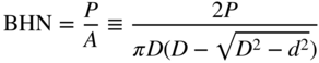
where A (in mm2) is the spherical surface area and d (in mm) is the diameter of the crater or indentation formed. The diameter d and the depth h of indentation are related by (Figure 2.13b)
(2.80)

Figure 2.13 Brinell hardness test.
It is desired to find the size of indentation, in terms of the values of d and h, when a tungsten carbide ball indenter of diameter 10 mm is used under a load of P = 3000 kgf on a stainless steel test specimen of BHN 1250. Find the values of d and h by formulating and solving the problem as an unconstrained minimization problem.
Hint: Consider the objective function as the sum of squares of the equations implied by Eqs. (2.79) and (2.80).
- 2.60 A manufacturer produces small refrigerators at a cost of $60 per unit and sells them to a retailer in a lot consisting of a minimum of 100 units. The selling price is set at $80 per unit if the retailer buys 100 units at a time. If the retailer buys more than 100 units at a time, the manufacturer agrees to reduce the price of all refrigerators by 10 cents for each unit bought over 100 units. Determine the number of units to be sold to the retailer to maximize the profit of the manufacturer.
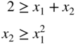
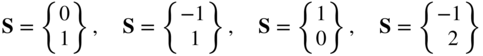
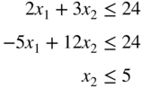
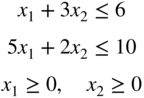
- 2.61 Consider the following problem:

subject to
Using Kuhn–Tucker conditions, find which of the following vectors are local minima:

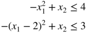
- 2.62 Using Kuhn–Tucker conditions, find the value(s) of β for which the point
 will be optimal to the problem:

subject to

Verify your result using a graphical procedure.
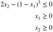
- 63 Consider the following optimization problem:

subject to
- (63) (63) Find whether the design vector X = {1, 1}T satisfies the Kuhn–Tucker conditions for a constrained optimum.
- (63) (63) What are the values of the Lagrange multipliers at the given design vector?
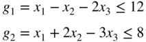
- 2.64 Consider the following problem:

subject to

Determine whether the Kuhn–Tucker conditions are satisfied at the following points:

- 2.65 Find a usable and feasible direction S at (a) X
1 = {−1, 5}T and (b) X
2 = {2, 3}T for the following problem:

subject to
- 2.66 Consider the following problem:

subject to
Determine whether the following search direction is usable, feasible, or both at the design vector
 :
:
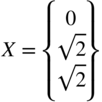
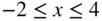
- 2.67 Consider the following problem:

subject to

Determine whether the following vector represents an optimum solution:
- 2.68

subject to the constraints
using Kuhn–Tucker conditions.
- 2.69

subject to
by (a) the graphical method and (b) Kuhn–Tucker conditions.
- 2.70

subject to
by applying Kuhn–Tucker conditions.
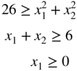
- 2.71 Consider the following problem:

subject to
Determine whether the constraint qualification and Kuhn–Tucker conditions are satisfied at the optimum point.
- 2.72 Consider the following problem:

subject to
Determine whether the constraint qualification and the Kuhn–Tucker conditions are satisfied at the optimum point.
- 2.73 Verify whether the following problem is convex:

subject to

- 74 Check the convexity of the following problems.
- (74) (74) subject to

- (74) (74)

subject to

- (74) (74)
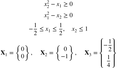
- 2.75 Identify the optimum point among the given design vectors, X
1, X
2, and X
3, by applying the Kuhn–Tucker conditions to the following problem:

subject to
- 2.76 Consider the following optimization problem:

subject to

Find a usable feasible direction at each of the following design vectors:
