
15
Practical Aspects of Optimization
15.1 Introduction
Although the mathematical techniques described earlier, particularly Chapters 3-13, can be used to solve different types of engineering optimization problems, the use of engineering judgment and approximations help in reducing the computational effort involved. In this chapter we consider several types of approximation techniques that can speed up the analysis time without introducing too much error [1]. The approximation methods include the reduction of size of an optimization problem, fast reanalysis techniques, and use of derivatives of static displacements and stresses, eigenvalues and eigenvectors, and transient response of mechanical and structural systems in gradient evaluations, and also in predicting the response in the neighborhood of a base design. These techniques are especially useful in finite element analysis‐based optimization procedures. This chapter presents several types of approximation methods that can be used in practical computation, and also the use of derivatives of different structural/mechanical system response quantities to speed up the optimization process.
15.2 Reduction of Size of an Optimization Problem
15.2.1 Reduced Basis Technique
In the optimum design of certain practical systems involving a large number of (n) design variables, some feasible design vectors X 1, X 2, …, X r may be available to start with. These design vectors may have been suggested by experienced designers or may be available from the design of similar systems in the past. We can reduce the size of the optimization problem by expressing the design vector X as a linear combination of the available feasible design vectors as
where c 1, c 2, …, c r are the unknown constants. Then the optimization problem can be solved using c 1, c 2, …, c r as design variables. This problem will have a much smaller number of unknowns since r ≪ n. In Eq. (15.1), the feasible design vectors X 1, X 2, …, X r serve as the basis vectors. It can be seen that if c 1 = c 2 = ⋯ = c r = 1/r, then X denotes the average of the basis vectors.
15.2.2 Design Variable Linking Technique
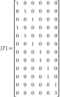
When the number of elements or members in a structure is large, it is possible to reduce the number of design variables by using a technique known as design variable linking [15.17]. To see this procedure, consider the 12‐member truss structure shown in Figure 15.1. If the area of cross section of each member is varied independently, we will have 12 design variables. On the other hand, if symmetry of members about the vertical (Y) axis is required, the areas of cross section of members 4, 5, 6, 8, and 10 can be assumed to be the same as those of members 1, 2, 3, 7, and 9, respectively. This reduces the number of independent design variables from 12 to 7. In addition, if the cross‐sectional area of member 12 is required to be three times that of member 11, we will have six independent design variables only:


Figure 15.1 Concept of design variable linking.
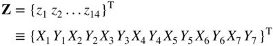
Once the vector X is known, the dependent variables can be determined as A 4 = A 1, A 5 = A 2, A 6 = A 3, A 8 = A 7, A 10 = A 9, and A 12 = 3A 11. This procedure of treating certain variables as dependent variables is known as design variable linking. By defining the vector of all variables as
the relationship between Z and X can be expressed as
where the matrix [T] is given by
The concept can be extended to many other situations. For example, if the geometry of the structure is to be varied during optimization (configuration optimization) while maintaining (i) symmetry about the Y axis and (ii) alignment of the three nodes 2, 3, and 4 (and 6, 7, and 4), we can define the following independent and dependent design variables:
Independent variables: X 5, X 6, Y 6, Y 7, Y 4
Dependent variables:

Thus the design vector X is

The relationship between the dependent and independent variables can be defined more systematically, by defining a vector of all geometry variables, Z, as
which is related to X through the relations
where f i denotes a function of X.
15.3 Fast Reanalysis Techniques
15.3.1 Incremental Response Approach
Let the displacement vector of the structure or machine, Y 0, corresponding to the load vector, P 0, be given by the solution of the equilibrium equations
or
where [K 0] is the stiffness matrix corresponding to the design vector, X 0. When the design vector is changed to X 0 + ΔX, let the stiffness matrix of the system change to [K 0] + [ΔK], the displacement vector to Y 0 + ΔY, and the load vector to P 0 + ΔP. The equilibrium equations at the new design vector, X 0 + ΔX, can be expressed as
or
Subtracting Eq. (15.7) from Eq. (15.10), we obtain
By neglecting the term [ΔK]ΔY, Eq. (15.11) can be reduced to
which yields the first approximation to the increment in displacement vector ΔY as
where [K 0]−1 is available from the solution in Eq. (15.8). We can find a better approximation of ΔY by subtracting Eq. (15.12) from Eq. (15.11):
or
By defining
Eq. (15.15) can be expressed as
Neglecting the term [ΔK] ΔY 2, Eq. (15.17) can be used to obtain the second approximation to ΔY, ΔY 2, as
From Eq. (15.16), ΔY can be written as

This process can be continued and ΔY can be expressed, in general, as

where ΔY i is found by solving the equations
Note that the series given by Eq. (15.20) may not converge if the change in the design vector, ΔX, is not small. Hence it is important to establish the validity of the procedure for each problem, by determining the step sizes for which the series will converge, before using it. The iterative process is usually stopped either by specifying a maximum number of iterations and/or by prescribing a convergence criterion such as

where ||ΔY i || is the Euclidean norm of the vector ΔY i and ε is a small number on the order of 0.01.
15.3.2 Basis Vector Approach
In structural optimization involving a static response, it is possible to conduct an approximate analysis at modified designs based on a limited number of exact analysis results. This results in a substantial saving in computer time, since, in most problems, the number of design variables is far smaller than the number of degrees of freedom of the system. Consider the equilibrium equations of the structure in the form
where [K] is the stiffness matrix, Y the vector of displacements, and P the load vector. Let the structure have n design variables denoted by the design vector

If we find the exact solution at r basic design vectors X 1, X 2, …, X r , the corresponding solutions, Y i , are found by solving the equations
where the stiffness matrix, [K i ], is determined at the design vector X i . If we consider a new design vector, X N , in the neighborhood of the basic design vectors, the equilibrium equations at X N can be expressed as
where [K N ] is the stiffness matrix evaluated at X N . By approximating Y N as a linear combination of the basic displacement vectors Y i , i = 1, 2, …, r, we have
where [Y] = [Y 1, Y 2, ⋯, Y r ] is an n × r matrix and c = {c 1, c 2, ⋯, c r }T is an r‐component column vector. Substitution of Eq. (15.26) into Eq. (15.25) gives
By premultiplying Eq. (15.27) by [Y]T we obtain
where
It can be seen that an approximate displacement vector Y N can be obtained by solving a smaller (r) system of equations, Eq. (15.28), instead of computing the exact solution Y N by solving a larger (n) system of equations, Eq. (15.25). The foregoing method is equivalent to applying the Ritz–Galerkin principle in the subspace spanned by the set of vectors Y 1, Y 2, …, Y r . The assumed modes Y i , i = 1, 2, …, r, can be considered to be good basis vectors since they are the solutions of similar sets of equations.
Fox and Miura [3] applied this method for the analysis of a 124‐member, 96‐degree‐of‐freedom space truss (shown in Figure 15.3). By using a 5‐degree‐of‐freedom approximation, they observed that the solution of Eq. (15.28) required 0.653 second while the solution of Eq. (15.25) required 5.454 seconds without exceeding 1% error in the maximum displacement components of the structure.

Figure 15.3 Space truss [3].
15.4 Derivatives of Static Displacements and Stresses
The gradient‐based optimization methods require the gradients of the objective and constraint functions. Thus the partial derivatives of the response quantities with respect to the design variables are required. Many practical applications require a finite‐element analysis for computing the values of the objective function and/or constraint functions at any design vector. Since the objective and/or constraint functions are to be evaluated at a large number of trial design vectors during optimization, the computation of the derivatives of the response quantities requires substantial computational effort. It is possible to derive approximate expressions for the response quantities. The derivatives of static displacements, stresses, eigenvalues, eigenvectors, and transient response of structural and mechanical systems are presented in this and the following two sections. The equilibrium equations of a machine or structure can be expressed as
where [K] is the stiffness matrix, Y the displacement vector, and P the load vector. By differentiating Eq. (15.31) with respect to the design variable x i , we obtain

where ∂[K]/∂x i denotes the matrix formed by differentiating the elements of [K] with respect to x i . Usually, the matrix is computed using a finite‐difference scheme as
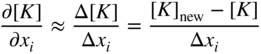
where [K]new is the stiffness matrix evaluated at the perturbed design vector X + ΔX i , where the vector ΔX i contains Δx i in the ith location and zero everywhere else:
In most cases the load vector P is either independent of the design variables or a known function of the design variables, and hence the derivatives, ∂ P /∂x i , can be evaluated with no difficulty. Equation (15.32) can be solved to find the derivatives of the displacements as

Since [K]−1 or its equivalent is available from the solution of Eqs. (15.31) and (15.35) can readily be solved to find the derivatives of static displacements with respect to the design variables.
The stresses in a machine or structure (in a particular finite element) can be determined using the relation
where [R] denotes the matrix that relates stresses to nodal displacements. The derivatives of stresses can then be computed as
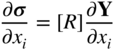
where the matrix [R] is usually independent of the design variables and the vector ∂ Y /∂x i is given by Eq. (15.35).
15.5 Derivatives of Eigenvalues and Eigenvectors
Let the eigenvalue problem be given by [4,6,10]
where λ is the eigenvalue, Y the eigenvector, [K] the stiffness matrix, and [M] the mass matrix corresponding to the design vector X = {x 1, x 2, ⋯, x n }T. Let the solution of Eq. (15.38) be given by the eigenvalues λ i and the eigenvectors Y i , i = 1, 2, …, m:
where [P i ] is a symmetric matrix given by
15.5.1 Derivatives of λ i
Premultiplication of Eq. (15.39) by ![]() gives
gives
Differentiation of Eq. (15.41) with respect to the design variable x j gives

where Y i,j = ∂ Y i /∂x j . In view of Eq. (15.39), Eq. (15.42) reduces to
Differentiation of Eq. (15.40) gives

where ∂[K]/∂x j and ∂[M]/∂x j denote the matrices formed by differentiating the elements of [K] and [M] matrices, respectively, with respect to x j . If the eigenvalues are normalized with respect to the mass matrix, we have [10]
Substituting Eq. (15.44) into Eq. (15.43) and using Eq. (15.45) gives the derivative of λ i with respect to x j as

It can be noted that Eq. (15.46) involves only the eigenvalue and eigenvector under consideration and hence the complete solution of the eigenvalue problem is not required to find the value of ∂λ i /∂x j .
15.5.2 Derivatives of Y i
The differentiation of Eqs. (15.39) and (15.45) with respect to x j results in


where ∂[P i ]/∂x j is given by Eq. (15.44). Equations (15.47) and (15.48) can be shown to be linearly independent and can be written together as

By premultiplying Eq. (15.49) by

we obtain
The solution of Eq. (15.50) gives the desired expression for the derivative of the eigenvector, ∂ Y i /∂x j , as
Again it can be seen that only the eigenvalue and eigenvector under consideration are involved in the evaluation of the derivatives of eigenvectors.
For illustration, a cylindrical cantilever beam is considered [4]. The beam is modeled with three finite elements with six degrees of freedom as indicated in Figure 15.4. The diameters of the beam are considered as the design variables, x i , i = 1, 2, 3. The first three eigenvalues and their derivatives are shown in Table 15.3 [4].

Figure 15.4 Cylindrical cantilever beam.
Table 15.3 Derivatives of eigenvalues [4].
| i | Eigenvalue, λ i |
|
|
|
|
| 1 | 24.66 | 0.3209 | −0.1582 | 1.478 | −2.298 |
| 2 | 974.7 | 3.86 | −0.4144 | 0.057 | −3.046 |
| 3 | 7782.0 | 23.5 | 21.67 | 0.335 | −5.307 |
15.6 Derivatives of Transient Response
The equations of motion of an n‐degree‐of‐freedom mechanical/structural system with viscous damping can be expressed as [10]
where [M], [C], and [K] are the n × n mass, damping, and stiffness matrices, respectively, F(t) is the n‐component force vector, Y is the n‐component displacement vector, and a dot over a symbol indicates differentiation with respect to time. Equation (15.52) denotes a set of n coupled second‐order differential equations. In most practical cases, n will be very large and Eq. (15.52) are stiff; hence the numerical solution of Eq. (15.52) will be tedious and produces an accurate solution only for low‐frequency components. To reduce the size of the problem, the displacement solution, Y, is expressed in terms of r basis functions Φ 1, Φ 2, …, and Φ r (with r ≪ n) as

where
is the matrix of basis functions, Φ jk the element in row j and column k of the matrix [Φ], q an r‐component vector of reduced coordinates, and q k (t) the kth component of the vector q. By substituting Eq. (15.53) into Eq. (15.52) and premultiplying the resulting equation by [Φ]T, we obtain a system of r differential equations:
where
Note that if the undamped natural modes of vibration are used as basis functions and if [C] is assumed to be a linear combination of [M] and [K] (called proportional damping), Eq. (15.54) represent a set of r uncoupled second‐order differential equations which can be solved independently [10]. Once q(t) is found, the displacement solution Y(t) can be determined from Eq. (15.53).
In the formulation of optimization problems with restrictions on the dynamic response, the constraints are placed on selected displacement components as
where y j is the displacement at location j on the machine/structure and y max is the maximum permissible value of the displacement. Constraints on dynamic stresses are also stated in a similar manner. Since Eq. (15.59) is a parametric constraint in terms of the parameter time (t), it is satisfied only at a set of peak or critical values of y j for computational simplicity. Once Eq. (15.59) is satisfied at the critical points, it will be satisfied (most likely) at all other values of t as well [11,12]. The values of y i at which dy j /dt = 0 or the values of y i at the end of the time interval denote local maxima and hence are to be considered as candidate critical points. Among the several candidate critical points, only a select number are considered for simplifying the computations. For example, in the response shown in Figure 15.5, peaks a, b, c, …, j qualify as candidate critical points. However, peaks a, b, f, and j can be discarded as their magnitudes are considerably smaller (less than, for example, 25%) than those of other peaks. Noting that peaks d and e (or g and h) represent essentially a single large peak with high‐frequency undulations, we can discard peak e (or g), which has a slightly smaller magnitude than d (or h). Thus finally, only peaks c, d, h, and i need to be considered to satisfy the constraint, Eq. (15.59).
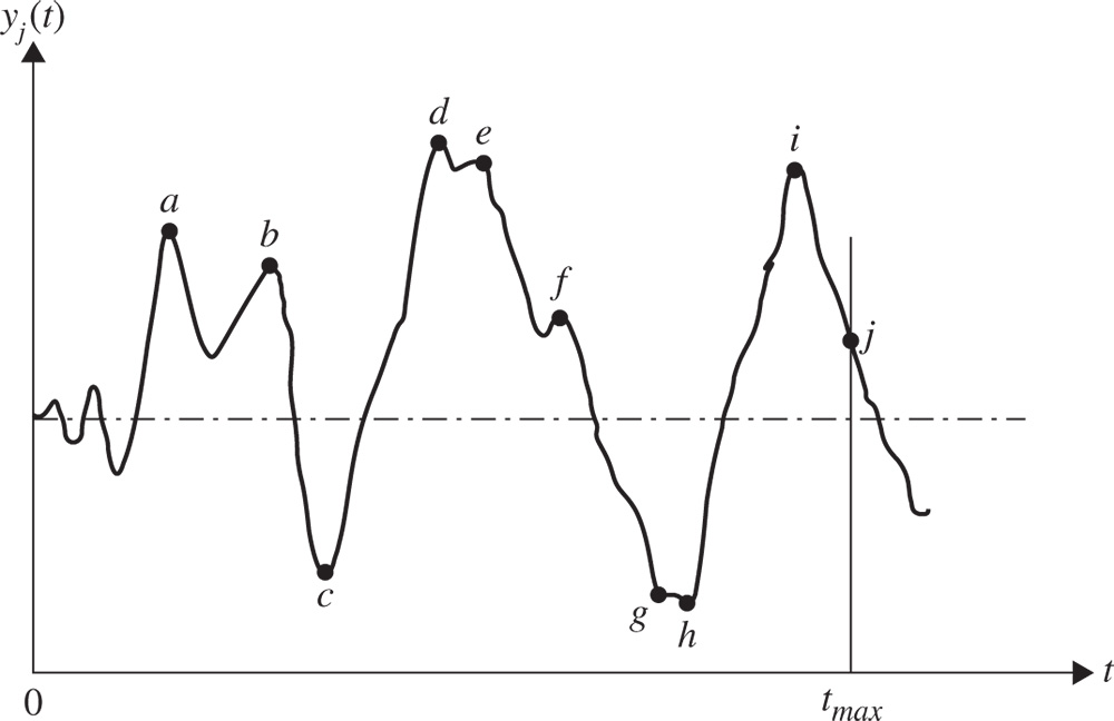
Figure 15.5 Critical points in a typical transient response.
Once the critical points are identified at a reference design X, the sensitivity of the response, y j (X, t) with respect to the design variable x i at the critical point t = t c can be found using the total derivative of y j as
The second term on the right‐hand side of Eq. (15.60) is always zero since ∂y j /∂t = 0 at an interior peak (0 < t c < t max) and dt c /dx i = 0 at the boundary (t c = t max). The derivative, ∂y j /∂x i , can be computed using Eq. (15.53) as
where, for simplicity, the elements of the matrix [Φ] are assumed to be constants (independent of the design vector X). Note that for higher accuracy, the derivatives of Φ jk with respect to x i (sensitivity of eigenvectors, if the mode shapes are used as the basis vectors) obtained from an equation similar to Eq. (15.51) can be included in finding ∂y j /∂x i .
To find the values of ∂q k /∂x i required in Eq. (15.61), Eq. (15.54) is differentiated with respect to x i to obtain

The derivatives of the matrices appearing on the right‐hand side of Eq. (15.62) can be computed using formulas such as

where, for simplicity, [Φ] is assumed to be constant and ∂[M]/∂x
i
is computed using a finite‐difference scheme. In most cases the forcing function F(t) will be known to be independent of X or an explicit function of X. Hence the quantity ∂
![]() /∂x
i
can be evaluated without much difficulty. Once the right‐hand side is known, Eq. (15.62) can be integrated numerically in time to find the values of ∂
/∂x
i
can be evaluated without much difficulty. Once the right‐hand side is known, Eq. (15.62) can be integrated numerically in time to find the values of ∂
![]() /∂x
i
, ∂
/∂x
i
, ∂
![]() /∂x
i
, and ∂
q
/∂x
i
. Using the values of ∂
q
/∂x
i
= {∂q
k
/∂x
i
} at the critical point t
c
, the required sensitivity of transient response can be found from Eq. (15.61).
/∂x
i
, and ∂
q
/∂x
i
. Using the values of ∂
q
/∂x
i
= {∂q
k
/∂x
i
} at the critical point t
c
, the required sensitivity of transient response can be found from Eq. (15.61).
15.7 Sensitivity of Optimum Solution to Problem Parameters
Any optimum design problem involves a design vector and a set of problem parameters (or preassigned parameters). In many cases, we would be interested in knowing the sensitivities or derivatives of the optimum design (design variables and objective function) with respect to the problem parameters [17,18]. As an example, consider the minimum weight design of a machine component or structure subject to a constraint on the induced stress. After solving the problem, we may wish to find the effect of changing the material. This means that we would like to know the changes in the optimal dimensions and the minimum weight of the component or structure due to a change in the value of the permissible stress. Usually, the sensitivity derivatives are found by using a finite‐difference method. But this requires a costly reoptimization of the problem using incremented values of the parameters. Hence, it is desirable to derive expressions for the sensitivity derivatives from appropriate equations. In this section we discuss two approaches: one based on the Kuhn–Tucker conditions and the other based on the concept of feasible direction.
15.7.1 Sensitivity Equations Using Kuhn–Tucker Conditions
The Kuhn–Tucker conditions satisfied at the constrained optimum design X * are given by [see Eqs. (2.73) and (2.74)]
where J
1 is the set of active constraints and Eqs. (15.64,15.65,15.66) are valid with X = X
* and λ
j
= ![]() . When a problem parameter changes by a small amount, we assume that Eqs. (15.64,15.65,15.66) remain valid. Treating f, g
j
, X, and λ
j
as functions of a typical problem parameter p, differentiation of Eqs. (15.64) and (15.65) with respect to p leads to
. When a problem parameter changes by a small amount, we assume that Eqs. (15.64,15.65,15.66) remain valid. Treating f, g
j
, X, and λ
j
as functions of a typical problem parameter p, differentiation of Eqs. (15.64) and (15.65) with respect to p leads to
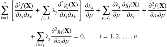

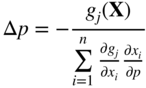
Equations (15.67) and (15.68) can be expressed in matrix form as
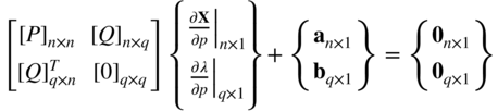
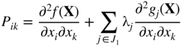
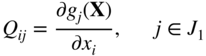
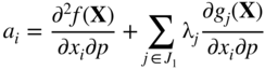
where q denotes the number of active constraints and the elements of the matrices and vectors in Eq. (15.69) are given by


The following can be noted in Eq. (15.69):
- Equation (15.69) denotes (n + q) simultaneous equations in terms of the required sensitivity derivatives, ∂x i /∂p (i = 1, 2, …, n) and ∂λ j /∂p (j = 1, 2, …, q). Both X * and λ* are assumed to be known in Eq. (15.69). If λ* are not computed during the optimization process, they can be computed using Eq. (7.263).
- Equation (15.69) can be solved only if the system is nonsingular. One of the requirements for this is that the active constraints be independent.
- Second derivatives of f and g j are required in computing the elements of [P] and a.
- If sensitivity derivatives are required with respect to several problem parameters p 1, p 2, …, only the vectors a and b need to be computed for each case and the system of Eq. (15.69) can be solved efficiently using the techniques of solving simultaneous equations with different right‐hand‐side vectors.
Once Eq. (15.69) are solved, the sensitivity of optimum objective value with respect to p can be computed as

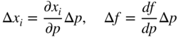
The changes in the optimum values of x i and f necessary to satisfy the Kuhn–Tucker conditions due to a change Δp in the problem parameter can be estimated as
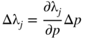
The changes in the values of Lagrange multiplier λ j due to Δp can be estimated as
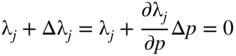
Equation (15.77) can be used to determine whether an originally active constraint becomes inactive due to the change, Δp. Since the value of λ j is zero for an inactive constraint, we have
from which the value of Δp necessary to make the jth constraint inactive can be found as

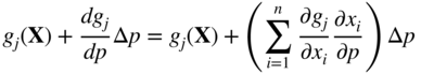
Similarly, a currently inactive constraint will become critical due to Δp if the new value of g j becomes zero:
Thus, the change Δp necessary to make an inactive constraint active can be found as
15.7.2 Sensitivity Equations Using the Concept of Feasible Direction
Here we treat the problem parameter p as a design variable so that the new design vector becomes
As in the case of the method of feasible directions (see Section 7.7), we formulate the direction finding problem as
subject to

where the gradients of f and g j (j ∈ J 1) can be evaluated in the usual manner. The set J 1 can also include nearly active constraints (along with the active constraints), so that we do not violate any constraint due to the change, Δp. The solution of the problem stated in Eq. (15.83) gives a usable feasible search direction, S. A new design vector along S can be expressed as
where λ is the step length and the components of S can be considered as

so that
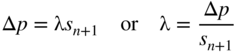
If the vector S is normalized by dividing its components by s n+1, Eq. (15.86) gives λ = Δp and hence Eq. (15.85) gives the desired sensitivity derivatives as
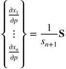
Thus the sensitivity of the objective function with respect to p can be computed as

Note that unlike the previous method, this method does not require the values of λ* and the second derivatives of f and g j to find the sensitivity derivatives. Also, if sensitivities with respect to several problem parameters p 1, p 2, … are required, all we need to do is to add them to the design vector X in Eq. (15.82).
References and Bibliography
- 1 Schmidt, L.A. Jr. and Farshi, B. (1974). Some approximation concepts for structural synthesis. AIAA Journal 12 (5): 692–699.
- 2 Haug, E.J., Choi, K.K., and Komkov, V. (1986). Design Sensitivity Analysis of Structural Systems. New York: Academic Press.
- 3 Fox, R.L. and Miura, H. (1971). An approximate analysis technique for design calculations. AIAA Journal 9 (1): 177–179.
- 4 Fox, R.L. and Kapoor, M.P. (1968). Rates of change of eigenvalues and eigenvectors. AIAA Journal 6 (12): 2426–2429.
- 5 Murthy, D.V. and Haftka, R.T. (1988). Derivatives of eigenvalues and eigenvectors of general complex matrix. International Journal for Numerical Methods in Engineering 26: 293–311.
- 6 Nelson, R.B. (1976). Simplified calculation of eigenvector derivatives. AIAA Journal 14: 1201–1205.
- 7 Rao, S.S. (1972). Rates of change of flutter Mach number and flutter frequency. AIAA Journal 10: 1526–1528.
- 8 Sutter, T.R., Camarda, C.J., Walsh, J.L., and Adelman, H.M. (1988). Comparison of several methods for the calculation of vibration mode shape derivatives. AIAA Journal 26 (12): 1506–1511.
- 9 Rao, S.S. (2018). The Finite Element Method in Engineering, 6e. Burlington, MA: Elsevier Butterworth Heinemann.
- 10 Rao, S.S. (2017). Mechanical Vibrations, 6e. Upper Saddle River, NJ: Pearson Prentice Hall.
- 11 Grandhi, R.V., Haftka, R.T., and Watson, L.T. (1986). Efficient identification of critical stresses in structures subjected to dynamic loads. Computers and Structures 22: 373–386.
- 12 Greene, W.H. and Haftka, R.T. (1989). Computational aspects of sensitivity calculations in transient structural analysis. Computers and Structures 32 (2): 433–443.
- 13 Kirsch, U., Reiss, M., and Shamir, U. (1972). Optimum design by partitioning into substructures. ASCE Journal of the Structural Division 98 (ST1): 249–267.
- 14 Schmit, L.A., Jr., and Miura, H. (1976). Approximation Concepts for Efficient Structural Synthesis, NASA CR‐2552.
- 15 Schmit, L.A. and Fleury, C. (1980). Structural synthesis by combining approximation concepts and dual methods. AIAA Journal 18: 1252–1260.
- 16 Pan, T.S., Rao, S.S., and Venkayya, V.B. (1990). Rates of change of closed‐loop eigenvalues and eigenvectors of actively controlled structures. International Journal for Numerical Methods in Engineering 30 (5): 1013–1028.
- 17 Vanderplaats, G.N. (1984). Numerical Optimization Techniques for Engineering Design with Applications. New York: McGraw‐Hill.
- 18 Sobieszczanski‐Sobieski, J., Barthelemy, J.F., and Riley, K.M. (1982). Sensitivity of optimum solutions to problem parameters. AIAA Journal 20: 1291–1299.
- 19 Kirsch, U. (1981). Optimum Structural Design. Concepts, Methods, and Applications. New York: McGraw‐Hill.
- 20 Haftka, R.T. and Gürdal, Z. (1992). Elements of Structural Optimization, 3e. Dordrecht, The Netherlands: Kluwer Academic.
Review Questions
- 15.1 What is a reduced basis technique?
- 15.2 State two methods of reducing the size of an optimization problem.
- 15.3 What is design variable linking? Can it always be used?
- 15.4 Under what condition(s) is the convergence of the quantity Σ i ΔY i in the fast reanalysis method ensured?
- 15.5 How do you compute the derivatives of the stiffness matrix with respect to a design variable, ∂[K]/∂x i ?
- 15.6
Answer true or false:
- The computation of the derivatives of a particular λ i requires other eigenvalues besides λ i .
- The derivatives of the ith eigenvector can be found without knowledge of the eigenvectors other than Y i .
- There is only one way to derive expressions for the sensitivity of optimal objective function with respect to problem parameters.
Problems
- 15.1 Consider the minimum‐volume design of the four‐bar truss shown in Figure 15.2 subject to a constraint on the vertical displacement of node 4. Let X 1 = {1, 1, 0.5, 0.5}T and X 2 = {0.5, 0.5, 1, 1}T be two design vectors, with x i denoting the area of cross section of bar i(i = 1, 2, 3, 4). By expressing the optimum design vectors as X = c 1 X 1 + c 2 X 2, determine the values of c 1 and c 2 through graphical optimization when the maximum permissible vertical deflection of node 4 is restricted to a magnitude of 0.1 in.
- 15.2
Consider the configuration (shape) optimization of the 10‐bar truss shown in Figure 15.6. The (X, Y) coordinates of the nodes are to be varied while maintaining (a) symmetry of the structure about the X axis, and (b) alignment of nodes 1, 2, and 3 (4, 5, and 6). Identify the independent and dependent design variables and derive the relevant design variable linking relationships.

Figure 15.6 Design variable linking of a 10‐bar truss. - 3 For the four‐bar truss considered in Example 15.1 (shown in Figure 15.2), a base design vector is given by X
0 = {A
1, A
2, A
3, A
4}T = {2.0, 1.0, 2.0, 1.0}T in.2. If ΔX is given by ΔX = {0.4, 0.4, −0.4, −0.4}T in.2, determine
- The exact displacement vector Y 0 = {y 5, y 6, y 7, y 8}T at X 0
- The exact displacement vector (Y 0 + ΔY) at (X 0 + ΔX)
- The displacement vector (Y 0 + ΔY) where ΔY is given by Eq. (14.20) with five terms
- 4 Consider the 11‐member truss shown in Figure 5.1 with loads Q = −1000 lb, R = 1000 lb, and S = 2000 lb. If A
i
= x
i
denotes the area of cross section of member i, and u
1, u
2, …, u
10 indicate the displacement components of the nodes, the equilibrium equations can be expressed as shown in Eqs. (E1)–(E10) of Example 5.1. Assuming that E = 30 × 106 psi, l = 50 in., x
i
= 1 in.2(i = 1, 2, …, 11), Δx
i
= 0.1 in.2(i = 1, 2, …, 5), and Δx
i
= −0.1 in.2(i = 6, 7, …, 11), determine
- Exact displacement solution U 0 at X 0
- Exact displacement solution (U 0 + ΔU) at the perturbed design, (X 0 + ΔX)
- Approximate displacement solution, (U 0 + ΔU), at(X 0 + ΔX) using Eq. (15.20) with four terms for ΔU
- 15.5 Consider the four‐bar truss shown in Figure 15.2 whose stiffness matrix is given by Eq. (E2) of Example 15.1. Determine the values of the derivatives of y i with respect to the area A 1, ∂y i /∂x 1 (i = 5, 6, 7, 8) at the reference design X 0 = {A 1 A 2 A 3 A 4}T = {2.0, 2.0, 1.0, 1.0}T in.2.
- 15.6 Find the values of ∂y i / ∂x 2 (i = 5, 6, 7, 8) in Problem 5.
- 15.7 Find the values of ∂y i / ∂x 3 (i = 5, 6, 7, 8) in Problem 5.
- 15.8 Find the values of ∂y i / ∂x 4 (i = 5, 6, 7, 8) in Problem 5.
- 9 The equilibrium equations of the stepped bar shown in Figure 15.7 are given by
(1)1

with
(2)2 (3)3
(3)3
If A 1 = 2 in.2, A 2 = 1 in.2, E 1 = E 2 = 30 × 106 psi, 2 l 1 = l 2 = 50 in., P 1 = 100 lb, and P 2 = 200 lb, determine
- Displacements, Y
- Values of ∂ Y /∂A 1 and ∂ Y /∂A 2 using the method of Section 15.4
-
Values of ∂σ/∂A
1 and ∂σ/∂A
2, where
σ
= {σ
1, σ
2}T denotes the vector of stresses in the bars and σ
1 = E
1
Y
1
/l
1 and σ
2 = E
2(Y
2 − Y
1)/l
2

Figure 15.7 Stepped bar.
- 10 The eigenvalue problem for the stepped bar shown in Figure 15.7 can be expressed as [K]Y = λ[M]Y with the mass matrix, [M], given by
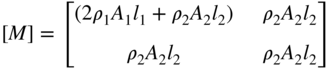
where ρ i , A i , and l i denote the mass density, area of cross section, and length of the segment i, and the stiffness matrix, [K], is given by Eq. (2) of Problem 9. If A 1 = 2 in.2, A 2 = 1 in.2, E 1 = E 2 = 30 × 106 psi, 2 l 1 = l 2 = 50 in., and ρ 1 g = ρ 2 g = 0.283 lb/in.3, determine
- Eigenvalues λ i and the eigenvectors Y i , i = 1, 2
- Values of ∂λ i /∂A 1, i = 1, 2, using the method of Section 15.5
- Values of ∂ Y i /∂ Y 1, i = 1, 2, using the method of Section 15.5
- 11 For the stepped bar considered in Problem 10, determine the following using the method of Section 15.5.
- Values of ∂λ i /∂A 2, i = 1, 2
- Values of ∂ Y i /∂A 2, i = 1, 2
- 15.12 A cantilever beam with a hollow circular section with outside diameter d and wall thickness t (Figure 15.8) is modeled with one beam finite element. The resulting static equilibrium equations can be expressed as

where I is the area moment of inertia of the cross section, E is Young's modulus, and l the length. Determine the displacements, Y i , and the sensitivities of the deflections, ∂Y i /∂d and ∂Y i /∂t(i = 1, 2), for the following data: E = 30 × 106 psi, l = 20 in., d = 2 in., t = 0.1 in., P 1 = 100 lb, and P 2 = 0.
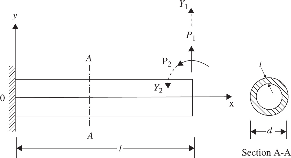
Figure 15.8 Hollow circular cantilever beam.
- 13 The eigenvalues of the cantilever beam shown in Figure 15.8 are governed by the equation

where E is Young's modulus, I the area moment of inertia, l the length, ρ the mass density, A the cross‐sectional area, λ the eigenvalue, and Y = {Y 1, Y 2}T = eigenvector. If E = 30 × 106 psi, d = 2 in., t = 0.1 in., l = 20 in., and ρg = 0.283 lb/in.3, determine
- Eigenvalues λ i and eigenvectors Y i (i = 1, 2)
- Values of ∂λ i /∂d and ∂λ i /∂t (i = 1, 2)
- 15.14 In Problem 13, determine the derivatives of the eigenvectors ∂ Y i /∂d and ∂ Y i /∂t(i = 1, 2).
- 15.15 The natural frequencies of the spring–mass system shown in Figure 15.9 are given by (for k
i
= k, i = 1, 2, 3 and m
i
= m, i = 1, 2)
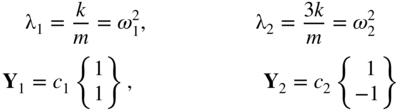
where ω 1 and ω 2 are the natural frequencies of vibration of the system and c 1 and c 2 are constants. The stiffness of each helical spring is given by

where d is the wire diameter, D the coil diameter, G the shear modulus, and n the number of turns of the spring. Determine the values of ∂ω i /∂D and ∂ Y i /∂D for the following data: d = 0.04 in., G = 11.5 × 10⁶ psi, D = 0.4 in., n = 10, and m = 32.2 lb ‐s 2/in. The stiffness and mass matrices of the system are given by
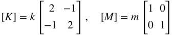

Figure 15.9 Two‐degree‐of‐freedom spring–mass system.
- 15.16
Find the sensitivities of
 ,
,  , and f
* with respect to Young's modulus of the tubular column considered in Example 1.1.
, and f
* with respect to Young's modulus of the tubular column considered in Example 1.1.