
3
Linear Programming I: Simplex Method
3.1 Introduction
Linear programming ( LP ) is an optimization method applicable for the solution of problems in which the objective function and the constraints appear as linear functions of the decision variables [1–8]. The constraint equations in a linear programming problem may be in the form of equalities or inequalities. The linear programming type of optimization problem was first recognized in the 1930s by economists while developing methods for the optimal allocation of resources. During World War II the U.S. Air Force sought more effective procedures of allocating resources and turned to linear programming. George B. Dantzig, who was a member of the Air Force group, formulated the general linear programming problem and devised the simplex method of solution in 1947 [1]. This has become a significant step in bringing linear programming into wider use. Afterward, much progress was made in the theoretical development and in the practical applications of linear programming. Among all the works, the theoretical contributions made by Kuhn and Tucker had a major impact in the development of the duality theory in LP. The works of Charnes and Cooper were responsible for industrial applications of LP.
Linear programming is considered a revolutionary development that permits us to make optimal decisions in complex situations. At least four Nobel Prizes were awarded for contributions related to linear programming. For example, when the Nobel Prize in Economics was awarded in 1975 jointly to L.V. Kantorovich of the former Soviet Union and T.C. Koopmans of the United States, the citation for the prize mentioned their contributions on the application of LP to the economic problem of allocating resources [9–11]. George Dantzig, the inventor of LP, was awarded the National Medal of Science by President Gerald Ford in 1976.
Although several other methods have been developed over the years for solving LP problems, the simplex method continues to be the most efficient and popular method for solving general LP problems. Among other methods, Karmarkar's method, developed in 1984, has been shown to be up to 50 times as fast as the simplex algorithm of Dantzig [12]. In this chapter we present the theory, development, and applications of the simplex method for solving LP problems. Additional topics, such as the revised simplex method, duality theory, decomposition method, postoptimality analysis, and Karmarkar's method, are considered in Chapter 4.
3.2 Applications of Linear Programming
The number of applications of linear programming has been so large that it is not possible to describe all of them here [13–17]. Only the early applications are mentioned here and the exercises at the end of this chapter give additional example applications of linear programming. One of the early industrial applications of linear programming was made in the petroleum refineries. In general, an oil refinery has a choice of buying crude oil from several different sources with differing compositions and at differing prices. It can manufacture different products, such as aviation fuel, diesel fuel, and gasoline, in varying quantities. The constraints may be due to the restrictions on the quantity of the crude oil available from a particular source, the capacity of the refinery to produce a particular product, and so on. A mix of the purchased crude oil and the manufactured products is sought that gives the maximum profit.
The optimal production plan in a manufacturing firm can also be decided using linear programming. Since the sales of a firm fluctuate, the company can have various options. It can build up an inventory of the manufactured products to carry it through the period of peak sales, but this involves an inventory holding cost. It can also pay overtime rates to achieve higher production during periods of higher demand. Finally, the firm need not meet the extra sales demand during the peak sales period, thus losing a potential profit. Linear programming can take into account the various cost and loss factors and arrive at the most profitable production plan.
In the food‐processing industry, linear programming has been used to determine the optimal shipping plan for the distribution of a particular product from different manufacturing plants to various warehouses. In the iron and steel industry, linear programming is used to decide the types of products to be made in their rolling mills to maximize the profit. Metalworking industries use linear programming for shop loading and for determining the choice between producing and buying a part. Paper mills use it to decrease the amount of trim losses. The optimal routing of messages in a communication network and the routing of aircraft and ships can also be decided using linear programming.
Linear programming has also been applied to formulate and solve several types of engineering design problems, such as the plastic design of frame structures, as illustrated in the following example.
3.3 Standard form of a Linear Programming Problem
The general linear programming problem can be stated in the following standard forms:
3.3.1 Scalar Form
subject to the constraints


where c j , b j , and a ij (i = 1, 2, …, m; j = 1, 2, …, n) are known constants, and x j are the decision variables.
3.3.2 Matrix Form
subject to the constraints
where
The characteristics of a linear programming problem, stated in standard form, are
- The objective function is of the minimization type.
- All the constraints are of the equality type.
- All the decision variables are nonnegative.
It is now shown that any linear programming problem can be expressed in standard form by using the following transformations.
- The maximization of a function f (x
1, x
2, …, x
n
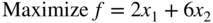
) is equivalent to the minimization of the negative of the same function. For example, the objective function

is equivalent to

Consequently, the objective function can be stated in the minimization form in any linear programming problem.
- In most engineering optimization problems, the decision variables represent some physical dimensions, and hence the variables x
j
will be nonnegative. However, a variable may be unrestricted in sign in some problems. In such cases, an unrestricted variable (which can take a positive, negative, or zero value) can be written as the difference of two nonnegative variables. Thus, if x
j
is unrestricted in sign, it can be written as
 , where
It can be seen that x j will be negative, zero, or positive, depending on whether
 is greater than, equal to, or less than
  .
. - If a constraint appears in the form of a “less than or equal to” type of inequality as

it can be converted into the equality form by adding a nonnegative slack variable x n+1 as follows:

Similarly, if the constraint is in the form of a “greater than or equal to” type of inequality as

it can be converted into the equality form by subtracting a variable as

where x n+1 is a nonnegative variable known as a surplus variable.
It can be seen that there are m equations in n decision variables in a linear programming problem. We can assume that m < n; for if m > n, there would be m − n redundant equations that could be eliminated. The case n = m is of no interest, for then there is either a unique solution X that satisfies Eqs. (3.2b) and (3.3b) (in which case there can be no optimization) or no solution, in which case the constraints are inconsistent. The case m < n corresponds to an underdetermined set of linear equations, which, if they have one solution, have an infinite number of solutions. The problem of linear programming is to find one of these solutions that satisfies Eqs. (3.2b) and (3.3b) and yields the minimum of f.
3.4 Geometry of Linear Programming Problems
A linear programming problem with only two variables presents a simple case for which the solution can be obtained by using a rather elementary graphical method. Apart from the solution, the graphical method gives a physical picture of certain geometrical characteristics of linear programming problems. The following example is considered to illustrate the graphical method of solution.
3.5 Definitions and Theorems
The geometrical characteristics of a linear programming problem stated in Section 3.4 can be proved mathematically. Some of the more powerful methods of solving linear programming problems take advantage of these characteristics. The terminology used in linear programming and some of the important theorems are presented in this section [1].
3.5.1 Definitions
- Point in n‐dimensional space. A point X in an n‐dimensional space is characterized by an ordered set of n values or coordinates (x 1, x 2, …, x n ). The coordinates of X are also called the components of X.
-
Line segment in n dimensions (L). If the coordinates of two points A and B are given by
 and
and  (j = 1, 2, …, n), the line segment (L) joining these points is the collection of points X(λ) whose coordinates are given by
  with 0 ≤ λ ≤ 1.
Thus
(3.4)
In one dimension, for example, it is easy to see that the definition is in accordance with our experience (Figure 3.7):
(3.5)
whence
(3.6)
-
Hyperplane. In n‐dimensional space, the set of points whose coordinates satisfy a linear equation
(3.7)

is called a hyperplane. A hyperplane, H, is represented as
(3.8)
A hyperplane has n − 1 dimensions in an n‐dimensional space. For example, in three‐dimensional space it is a plane, and in two‐dimensional space it is a line. The set of points whose coordinates satisfy a linear inequality like a 1 x 1 + ⋯ + a n x n ≤ b is called a closed half‐space, closed due to the inclusion of an equality sign in the inequality above. A hyperplane partitions the n‐dimensional space (E n ) into two closed half‐spaces, so that
(3.9) (3.10)
This is illustrated in Figure 3.8 in the case of a two‐dimensional space (E 2).
-
Convex set. A convex set is a collection of points such that if X
(1) and X
(2) are any two points in the collection, the line segment joining them is also in the collection. A convex set, S, can be defined mathematically as follows:

where

A set containing only one point is always considered to be convex. Some examples of convex sets in two dimensions are shown shaded in Figure 3.9. On the other hand, the sets depicted by the shaded region in Figure 3.10 are not convex. The L‐shaped region, for example, is not a convex set, because it is possible to find two points a and b in the set such that not all points on the line joining them belong to the set.
-
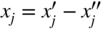
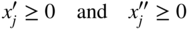
Convex polyhedron and convex polytope. A convex polyhedron is a set of points common to one or more half‐spaces. A convex polyhedron that is bounded is called a convex polytope.
Figure 3.11a and b represents convex polytopes in two and three dimensions, and Figure 3.11c and d denotes convex polyhedra in two and three dimensions. It can be seen that a convex polygon, shown in Figure 3.11a and c, can be considered as the intersection of one or more half‐planes.
- Vertex or extreme point. This is a point in the convex set that does not lie on a line segment joining two other points of the set. For example, every point on the circumference of a circle and each corner point of a polygon can be called a vertex or extreme point.
- Feasible solution. In a linear programming problem, any solution that satisfies the constraints (see Eqs. (3.2b) and (3.3b)) is called a feasible solution.
- Basic solution. A basic solution is one in which n − m variables are set equal to zero. A basic solution can be obtained by setting n − m variables to zero and solving the constraint Eq. (3.2b) simultaneously.
- Basis. The collection of variables not set equal to zero to obtain the basic solution is called the basis.
- Basic feasible solution. This is a basic solution that satisfies the nonnegativity conditions of Eq. (3.3b).
- Nondegenerate basic feasible solution. This is a basic feasible solution that has got exactly m positive x i .
- Optimal solution. A feasible solution that optimizes the objective function is called an optimal solution.
- Optimal basic solution. This is a basic feasible solution for which the objective function is optimal.

Figure 3.7 Line segment.

Figure 3.8 Hyperplane in two dimensions.

Figure 3.9 Convex sets.

Figure 3.10 Nonconvex sets.
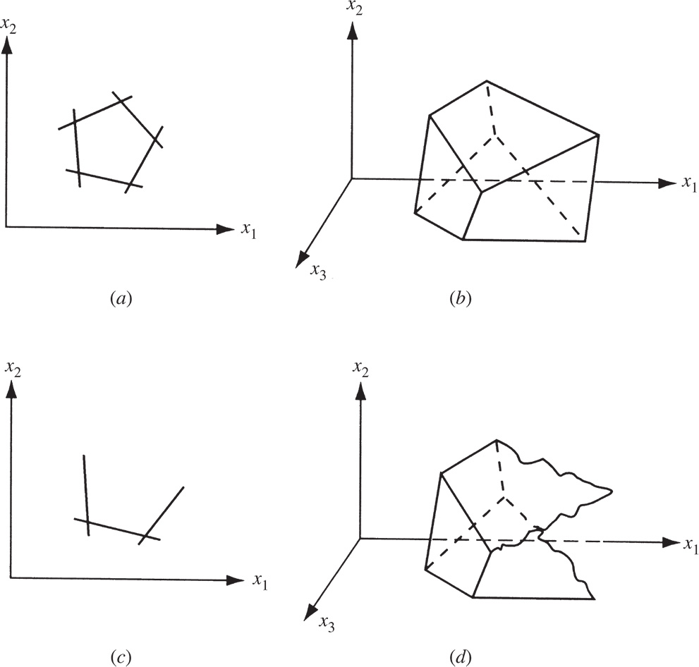
Figure 3.11 Convex polytopes in two and three dimensions (a, b) and convex polyhedra in two and three dimensions (c, d).
3.5.2 Theorems
The basic theorems of linear programming can now be stated and proved.2

Figure 3.12 Intersection of two convex sets.

Figure 3.13 Local and global minima.
The proofs of Theorems 3.4–3.6 can be found in Ref. [1].
3.6 Solution of a System of Linear Simultaneous Equations
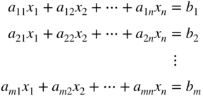
Before studying the most general method of solving a linear programming problem, it will be useful to review the methods of solving a system of linear equations. Hence, in the present section we review some of the elementary concepts of linear equations. Consider the following system of n equations in n unknowns:

Assuming that this set of equations possesses a unique solution, a method of solving the system consists of reducing the equations to a form known as canonical form.
It is well known from elementary algebra that the solution of Eq. (3.14) will not be altered under the following elementary operations: (i) any equation E r is replaced by the equation kE r , where k is a nonzero constant, and (ii) any equation E r is replaced by the equation E r + kE s , where E s is any other equation of the system. By making use of these elementary operations, the system of Eq. (3.14) can be reduced to a convenient equivalent form as follows. Let us select some variable x i and try to eliminate it from all the equations except the jth one (for which a ji is nonzero). This can be accomplished by dividing the jth equation by a ji and subtracting a ki times the result from each of the other equations, k = 1, 2, …, j − 1, j + 1, …, n. The resulting system of equations can be written as
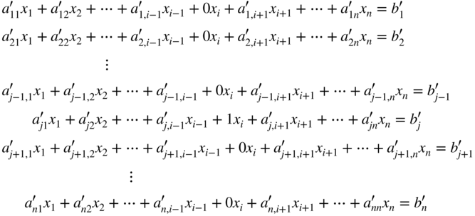
where the primes indicate that the ![]() and
and ![]() are changed from the original system. This procedure of eliminating a particular variable from all but one equation is called a pivot operation. The system of Eq. (3.15) produced by the pivot operation have exactly the same solution as the original set of Eq. (3.14). That is, the vector X that satisfies Eq. 3.14 satisfies Eq. (3.15), and vice versa.
are changed from the original system. This procedure of eliminating a particular variable from all but one equation is called a pivot operation. The system of Eq. (3.15) produced by the pivot operation have exactly the same solution as the original set of Eq. (3.14). That is, the vector X that satisfies Eq. 3.14 satisfies Eq. (3.15), and vice versa.
Next time, if we take the system of Eq. (3.15) and perform a new pivot operation by eliminating x s , s ≠ i, in all the equations except the tth equation, t ≠ j, the zeros or the 1 in the ith column will not be disturbed. The pivotal operations can be repeated by using a different variable and equation each time until the system of Eq. (3.14) is reduced to the form

This system of Eq. (3.16) is said to be in canonical form and has been obtained after carrying out n pivot operations. From the canonical form, the solution vector can be directly obtained as
Since the set of Eq. (3.16) has been obtained from Eq. (3.14) only through elementary operations, the system of Eq. (3.16) is equivalent to the system of Eq. (3.14). Thus, the solution given by Eq. (3.17) is the desired solution of Eq. 3.14.
3.7 Pivotal Reduction of a General System of Equations
Instead of a square system, let us consider a system of m equations in n variables with n ≥ m. This system of equations is assumed to be consistent so that it will have at least one solution:
The solution vector(s) X that satisfy Eq. (3.18) are not evident from the equations. However, it is possible to reduce this system to an equivalent canonical system from which at least one solution can readily be deduced. If pivotal operations with respect to any set of m variables, say, x 1, x 2, …, x m , are carried, the resulting set of equations can be written as follows:

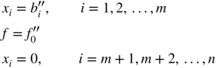
One special solution that can always be deduced from the system of Eq. (3.19) is

This solution is called a basic solution since the solution vector contains no more than m nonzero terms. The pivotal variables x
i
, i = 1, 2, …, m, are called the basic variables and the other variables x
i
, i = m + 1, m + 2, …, n, are called the nonbasic variables. Of course, this is not the only solution, but it is the one most readily deduced from Eq. (3.19). If all ![]() i = 1, 2, …, m, in the solution given by Eq. (3.20) are nonnegative, it satisfies Eq. (3.3b) in addition to Eq. (3.2b), and hence it can be called a basic feasible solution.
i = 1, 2, …, m, in the solution given by Eq. (3.20) are nonnegative, it satisfies Eq. (3.3b) in addition to Eq. (3.2b), and hence it can be called a basic feasible solution.
It is possible to obtain the other basic solutions from the canonical system of Eq. (3.19). We can perform an additional pivotal operation on the system after it is in canonical form, by choosing ![]() (which is nonzero) as the pivot term, q > m, and using any row p (among 1, 2, …, m). The new system will still be in canonical form but with x
q
as the pivotal variable in place of x
p
. The variable x
p
, which was a basic variable in the original canonical form, will no longer be a basic variable in the new canonical form. This new canonical system yields a new basic solution (which may or may not be feasible) similar to that of Eq. (3.20). It is to be noted that the values of all the basic variables change, in general, as we go from one basic solution to another, but only one zero variable (which is nonbasic in the original canonical form) becomes nonzero (which is basic in the new canonical system), and vice versa.
(which is nonzero) as the pivot term, q > m, and using any row p (among 1, 2, …, m). The new system will still be in canonical form but with x
q
as the pivotal variable in place of x
p
. The variable x
p
, which was a basic variable in the original canonical form, will no longer be a basic variable in the new canonical form. This new canonical system yields a new basic solution (which may or may not be feasible) similar to that of Eq. (3.20). It is to be noted that the values of all the basic variables change, in general, as we go from one basic solution to another, but only one zero variable (which is nonbasic in the original canonical form) becomes nonzero (which is basic in the new canonical system), and vice versa.
3.8 Motivation of the Simplex Method
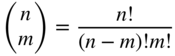
Given a system in canonical form corresponding to a basic solution, we have seen how to move to a neighboring basic solution by a pivot operation. Thus, one way to find the optimal solution of the given linear programming problem is to generate all the basic solutions and pick the one that is feasible and corresponds to the optimal value of the objective function. This can be done because the optimal solution, if one exists, always occurs at an extreme point or vertex of the feasible domain. If there are m equality constraints in n variables with n ≥ m, a basic solution can be obtained by setting any of the n − m variables equal to zero. The number of basic solutions to be inspected is thus equal to the number of ways in which m variables can be selected from a set of n variables, that is,
For example, if n = 10 and m = 5, we have 252 basic solutions, and if n = 20 and m = 10, we have 184 756 basic solutions. Usually, we do not have to inspect all these basic solutions since many of them will be infeasible. However, for large values of n and m, this is still a very large number to inspect one by one. Hence, what we really need is a computational scheme that examines a sequence of basic feasible solutions, each of which corresponds to a lower value of f until a minimum is reached. The simplex method of Dantzig is a powerful scheme for obtaining a basic feasible solution; if the solution is not optimal, the method provides for finding a neighboring basic feasible solution that has a lower or equal value of f. The process is repeated until, in a finite number of steps, an optimum is found.
The first step involved in the simplex method is to construct an auxiliary problem by introducing certain variables known as artificial variables into the standard form of the linear programming problem. The primary aim of adding the artificial variables is to bring the resulting auxiliary problem into a canonical form from which its basic feasible solution can be obtained immediately. Starting from this canonical form, the optimal solution of the original linear programming problem is sought in two phases. The first phase is intended to find a basic feasible solution to the original linear programming problem. It consists of a sequence of pivot operations that produces a succession of different canonical forms from which the optimal solution of the auxiliary problem can be found. This also enables us to find a basic feasible solution, if one exists, to the original linear programming problem. The second phase is intended to find the optimal solution to the original linear programming problem. It consists of a second sequence of pivot operations that enables us to move from one basic feasible solution to the next of the original linear programming problem. In this process, the optimal solution to the problem, if one exists, will be identified. The sequence of different canonical forms that is necessary in both the phases of the simplex method is generated according to the simplex algorithm described in the next section. That is, the simplex algorithm forms the main subroutine of the simplex method.
3.9 Simplex Algorithm
The starting point of the simplex algorithm is always a set of equations, which includes the objective function along with the equality constraints of the problem in canonical form. Thus the objective of the simplex algorithm is to find the vector X ≥ 0 that minimizes the function f (X) and satisfies the equations:
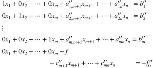
where ![]() , and
, and ![]() are constants. Notice that (−f) is treated as a basic variable in the canonical form of Eq. (3.21). The basic solution that can readily be deduced from Eq. (3.21) is
are constants. Notice that (−f) is treated as a basic variable in the canonical form of Eq. (3.21). The basic solution that can readily be deduced from Eq. (3.21) is
If the basic solution is also feasible, the values of x i , i = 1, 2, …, n, are nonnegative and hence
In phase I of the simplex method, the basic solution corresponding to the canonical form obtained after the introduction of the artificial variables will be feasible for the auxiliary problem. As stated earlier, phase II of the simplex method starts with a basic feasible solution of the original linear programming problem. Hence the initial canonical form at the start of the simplex algorithm will always be a basic feasible solution.
We know from Theorem 3.6 that the optimal solution of a linear programming problem lies at one of the basic feasible solutions. Since the simplex algorithm is intended to move from one basic feasible solution to the other through pivotal operations, before moving to the next basic feasible solution, we have to make sure that the present basic feasible solution is not the optimal solution. By merely glancing at the numbers ![]() , j = 1, 2, …, n, we can tell whether or not the present basic feasible solution is optimal. Theorem 3.7 provides a means of identifying the optimal point.
, j = 1, 2, …, n, we can tell whether or not the present basic feasible solution is optimal. Theorem 3.7 provides a means of identifying the optimal point.
3.9.1 Identifying an Optimal Point
3.9.2 Improving a Nonoptimal Basic Feasible Solution
From the last row of Eq. (3.21), we can write the objective function as
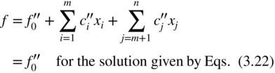
If at least one ![]() is negative, the value of f can be reduced by making the corresponding x
j
> 0. In other words, the nonbasic variable x
j
, for which the cost coefficient
is negative, the value of f can be reduced by making the corresponding x
j
> 0. In other words, the nonbasic variable x
j
, for which the cost coefficient ![]() is negative, is to be made a basic variable in order to reduce the value of the objective function. At the same time, due to the pivotal operation, one of the current basic variables will become nonbasic and hence the values of the new basic variables are to be adjusted in order to bring the value of f less than
is negative, is to be made a basic variable in order to reduce the value of the objective function. At the same time, due to the pivotal operation, one of the current basic variables will become nonbasic and hence the values of the new basic variables are to be adjusted in order to bring the value of f less than ![]() . If there are more than one
. If there are more than one ![]() the index s of the nonbasic variable x
s
which is to be made basic is chosen such that
the index s of the nonbasic variable x
s
which is to be made basic is chosen such that
Although this may not lead to the greatest possible decrease in f (since it may not be possible to increase x
s
very far), this is intuitively at least a good rule for choosing the variable to become basic. It is the one generally used in practice, because it is simple and it usually leads to fewer iterations than just choosing any ![]() . If there is a tie‐in applying Eq. (3.26), (i.e. if more than one
. If there is a tie‐in applying Eq. (3.26), (i.e. if more than one ![]() has the same minimum value), we select one of them arbitrarily as
has the same minimum value), we select one of them arbitrarily as ![]() .
.
Having decided on the variable x s to become basic, we increase it from zero, holding all other nonbasic variables zero, and observe the effect on the current basic variables. From Eq. (3.21), we can obtain


Since ![]() Eq. (3.28) suggests that the value of x
s
should be made as large as possible in order to reduce the value of f as much as possible. However, in the process of increasing the value of x
s
, some of the variables x
i
(i = 1, 2, …, m) in Eq. (3.27) may become negative. It can be seen that if all the coefficients
Eq. (3.28) suggests that the value of x
s
should be made as large as possible in order to reduce the value of f as much as possible. However, in the process of increasing the value of x
s
, some of the variables x
i
(i = 1, 2, …, m) in Eq. (3.27) may become negative. It can be seen that if all the coefficients ![]() i = 1, 2, …, m, then x
s
can be made infinitely large without making any x
i
< 0, i = 1, 2, …, m. In such a case, the minimum value of f is minus infinity and the linear programming problem is said to have an unbounded solution.
i = 1, 2, …, m, then x
s
can be made infinitely large without making any x
i
< 0, i = 1, 2, …, m. In such a case, the minimum value of f is minus infinity and the linear programming problem is said to have an unbounded solution.
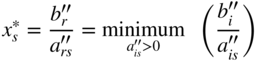
On the other hand, if at least one ![]() is positive, the maximum value that x
s
can take without making x
i
negative is
is positive, the maximum value that x
s
can take without making x
i
negative is ![]() . If there are more than one
. If there are more than one ![]() the largest value x
s
* that x
s
can take is given by the minimum of the ratios
the largest value x
s
* that x
s
can take is given by the minimum of the ratios ![]() for which
for which ![]() . Thus
. Thus
The choice of r in the case of a tie, assuming that all ![]() > 0, is arbitrary. If any
> 0, is arbitrary. If any ![]() for which
for which ![]() > 0 is zero in Eq. (3.27), x
s
cannot be increased by any amount. Such a solution is called a degenerate solution.
> 0 is zero in Eq. (3.27), x
s
cannot be increased by any amount. Such a solution is called a degenerate solution.
In the case of a nondegenerate basic feasible solution, a new basic feasible solution can be constructed with a lower value of the objective function as follows. By substituting the value of ![]() given by Eq. (3.29) into Eqs. (3.27) and (3.28), we obtain
given by Eq. (3.29) into Eqs. (3.27) and (3.28), we obtain
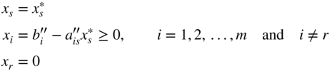

which can readily be seen to be a feasible solution different from the previous one. Since ![]() in Eq. (3.29), a single pivot operation on the element
in Eq. (3.29), a single pivot operation on the element ![]() in the system of Eq. (3.21) will lead to a new canonical form from which the basic feasible solution of Eq. (3.30) can easily be deduced. Also, Eq. (3.31) shows that this basic feasible solution corresponds to a lower objective function value compared to that of Eq. (3.22). This basic feasible solution can again be tested for optimality by seeing whether all
in the system of Eq. (3.21) will lead to a new canonical form from which the basic feasible solution of Eq. (3.30) can easily be deduced. Also, Eq. (3.31) shows that this basic feasible solution corresponds to a lower objective function value compared to that of Eq. (3.22). This basic feasible solution can again be tested for optimality by seeing whether all ![]() in the new canonical form. If the solution is not optimal, the entire procedure of moving to another basic feasible solution from the present one has to be repeated. In the simplex algorithm, this procedure is repeated in an iterative manner until the algorithm finds either (i) a class of feasible solutions for which f → −∞ or (ii) an optimal basic feasible solution with all
in the new canonical form. If the solution is not optimal, the entire procedure of moving to another basic feasible solution from the present one has to be repeated. In the simplex algorithm, this procedure is repeated in an iterative manner until the algorithm finds either (i) a class of feasible solutions for which f → −∞ or (ii) an optimal basic feasible solution with all ![]() i = 1, 2, …, n. Since there are only a finite number of ways to choose a set of m basic variables out of n variables, the iterative process of the simplex algorithm will terminate in a finite number of cycles. The iterative process of the simplex algorithm is shown as a flowchart in Figure 3.14.
i = 1, 2, …, n. Since there are only a finite number of ways to choose a set of m basic variables out of n variables, the iterative process of the simplex algorithm will terminate in a finite number of cycles. The iterative process of the simplex algorithm is shown as a flowchart in Figure 3.14.

Figure 3.14 Flowchart for finding the optimal solution by the simplex algorithm.
3.10 Two Phases of the Simplex Method
The problem is to find nonnegative values for the variables x 1, x 2, …, x n that satisfy the equations

and minimize the objective function given by
The general problems encountered in solving this problem are
- An initial feasible canonical form may not be readily available. This is the case when the linear programming problem does not have slack variables for some of the equations or when the slack variables have negative coefficients.
- The problem may have redundancies and/or inconsistencies, and may not be solvable in nonnegative numbers.
The two‐phase simplex method can be used to solve the problem.
Phase I of the simplex method uses the simplex algorithm itself to find whether the linear programming problem has a feasible solution. If a feasible solution exists, it provides a basic feasible solution in canonical form ready to initiate phase II of the method. Phase II, in turn, uses the simplex algorithm to find whether the problem has a bounded optimum. If a bounded optimum exists, it finds the basic feasible solution that is optimal. The simplex method is described in the following steps.
- Arrange the original system of Eq. (3.32) so that all constant terms b i are positive or zero by changing, where necessary, the signs on both sides of any of the equations.
- Introduce to this system a set of artificial variables y
1, y
2, …, y
m
(which serve as basic variables in phase I), where each y
i
≥ 0, so that it becomes
(3.34)

Note that in Eq. (3.34), for a particular i, the a ij 's and the b i may be the negative of what they were in Eq. (3.32) because of step 1.
The objective function of Eq. (3.33) can be written as
(3.35)
-
Phase I of the method. Define a quantity w as the sum of the artificial variables
(3.36)

and use the simplex algorithm to find x i ≥ 0 (i = 1, 2, …, n) and y i ≥ 0 (i = 1, 2, …, m) which minimize w and satisfy Eqs. (3.34) and (3.35). Consequently, consider the array
(3.37)
This array is not in canonical form; however, it can be rewritten as a canonical system with basic variables y 1, y 2, …, y m , −f, and −w by subtracting the sum of the first m equations from the last to obtain the new system
(3.38)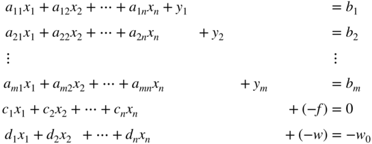
where
(3.39) (3.40)
Equation (3.38) provide the initial basic feasible solution that is necessary for starting phase I.
- In Eq. (3.37), the expression of w, in terms of the artificial variables y 1, y 2, …, y m is known as the infeasibility form. w has the property that if as a result of phase I, with a minimum of w > 0, no feasible solution exists for the original linear programming problem stated in Eqs. (3.32) and (3.33), and thus the procedure is terminated. On the other hand, if the minimum of w = 0, the resulting array will be in canonical form and hence initiate phase II by eliminating the w equation as well as the columns corresponding to each of the artificial variables y 1, y 2, …, y m from the array.
- Phase II of the method. Apply the simplex algorithm to the adjusted canonical system at the end of phase I to obtain a solution, if a finite one exists, which optimizes the value of f.
The flowchart for the two‐phase simplex method is given in Figure 3.15.
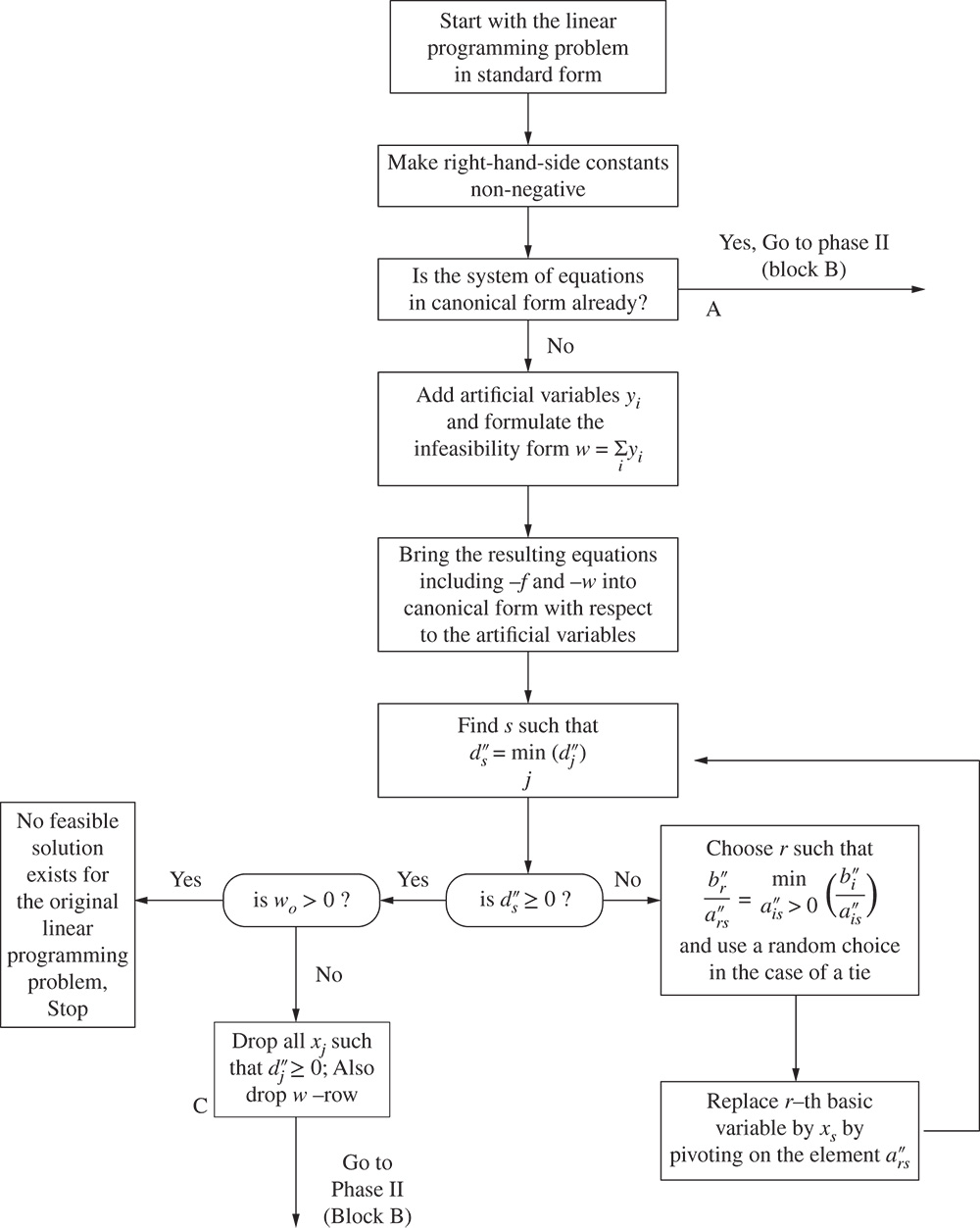
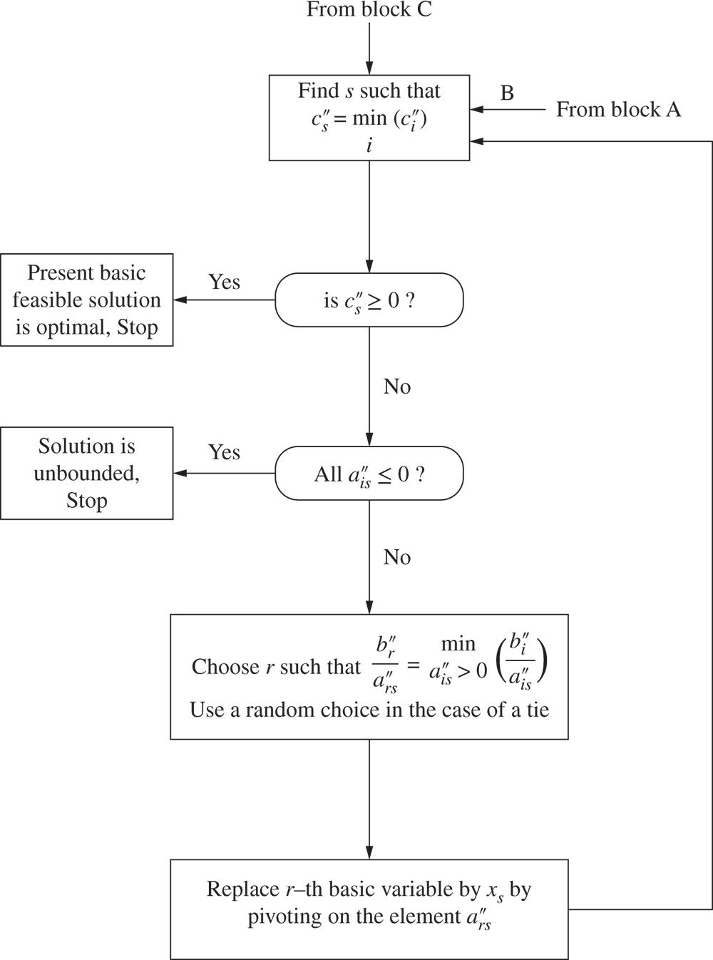
Figure 3.15 Flowchart for the two‐phase simplex method.
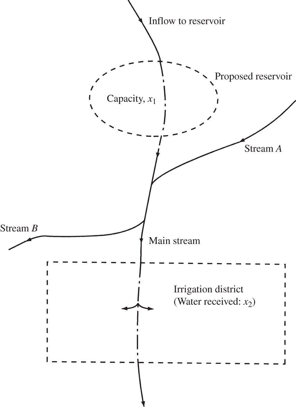
Figure 3.16 Reservoir in an irrigation district.

Figure 3.17 Scaffolding system with three beams.
3.11 Solutions Using MATLAB
The solution of different types of optimization problems using MATLAB is presented in Chapter 17. Specifically, the MATLAB solution of a linear programming problem is given in Example 17.3.
References and Bibliography
- 1 Dantzig, G.B. (1963). Linear Programming and Extensions. Princeton, NJ: Princeton University Press.
- 2 Adams, W.J., Gewirtz, A., and Quintas, L.V. (1969). Elements of Linear Programming. New York: Van Nostrand Reinhold.
- 3 Garvin, W.W. (1960). Introduction to Linear Programming. New York: McGraw‐Hill.
- 4 Gass, S.I. (1985). Linear Programming: Methods and Applications, 5e. New York: McGraw‐Hill.
- 5 Hadley, G. (1962). Linear Programming. Reading, MA: Addison‐Wesley.
- 6 Vajda, S. (1960). An Introduction to Linear Programming and the Theory of Games. New York: Wiley.
- 7 Orchard‐Hays, W. (1968). Advanced Linear Programming Computing Techniques. New York: McGraw‐Hill.
- 8 Gass, S.I. (1970). An Illustrated Guide to Linear Programming. New York: McGraw‐Hill.
- 9 Winston, W.L. (1991). Operations Research: Applications and Algorithms, 2e. Boston: PWS‐Kent.
- 10 Taha, H.A. (1992). Operations Research: An Introduction, 5e. New York: Macmillan.
- 11 Murty, K.G. (1983). Linear Programming. New York: Wiley.
- 12 Karmarkar, N. (1984). A new polynomial‐time algorithm for linear programming. Combinatorica 4 (4): 373–395.
- 13 Rubinstein, M.F. and Karagozian, J. (1966). Building design using linear programming. Journal of the Structural Division , Proceedings of ASCE 92 (ST6): 223–245.
- 14 Au, T. (1969). Introduction to Systems Engineering: Deterministic Models. Reading, MA: Addison‐Wesley.
- 15 Stoecker, W.F. (1989). Design of Thermal Systems, 3e. New York: McGraw‐Hill.
- 16 Stark, R.M. and Nicholls, R.L. (1972). Mathematical Foundations for Design: Civil Engineering Systems. New York: McGraw‐Hill.
- 17 Maass, A., Hufschmidt, M.A., Dorfman, R. et al. (1962). Design of Water Resources Systems. Cambridge, MA: Harvard University Press.
Review Questions
- 3.1 Define a line segment in n‐dimensional space.
- 3.2 What happens when m = n in a (standard) LP problem?
- 3.3 How many basic solutions can an LP problem have?
- 3.4 State an LP problem in standard form.
- 3.5 State four applications of linear programming.
- 3.6 Why is linear programming important in several types of industries?
- 3.7 Define the following terms: point, hyperplane, convex set, extreme point.
- 3.8 What is a basis?
- 3.9 What is a pivot operation?
- 3.10 What is the difference between a convex polyhedron and a convex polytope?
- 3.11 What is a basic degenerate solution?
- 3.12 What is the difference between the simplex algorithm and the simplex method?
- 3.13 How do you identify the optimum solution in the simplex method?
- 3.14 Define the infeasibility form.
- 3.15 What is the difference between a slack and a surplus variable?
- 3.16 Can a slack variable be part of the basis at the optimum solution of an LP problem?
- 3.17 Can an artificial variable be in the basis at the optimum point of an LP problem?
- 3.18 How do you detect an unbounded solution in the simplex procedure?
- 3.19 How do you identify the presence of multiple optima in the simplex method?
- 3.20 What is a canonical form?
- 21
Answer true or false:
- The feasible region of an LP problem is always bounded.
- An LP problem will have infinite solutions whenever a constraint is redundant.
- The optimum solution of an LP problem always lies at a vertex.
- A linear function is always convex.
- The feasible space of some LP problems can be nonconvex.
- The variables must be nonnegative in a standard LP problem.
- The optimal solution of an LP problem can be called the optimal basic solution.
- Every basic solution represents an extreme point of the convex set of feasible solutions.
- We can generate all the basic solutions of an LP problem using pivot operations.
- The simplex algorithm permits us to move from one basic solution to another basic solution.
- The slack and surplus variables can be unrestricted in sign.
- An LP problem will have an infinite number of feasible solutions.
- An LP problem will have an infinite number of basic feasible solutions.
- The right‐hand‐side constants can assume negative values during the simplex procedure.
- All the right‐hand‐side constants can be zero in an LP problem.
- The cost coefficient corresponding to a nonbasic variable can be positive in a basic feasible solution.
- If all elements in the pivot column are negative, the LP problem will not have a feasible solution.
- A basic degenerate solution can have negative values for some of the variables.
- If a greater‐than or equal‐to type of constraint is active at the optimum point, the corresponding surplus variable must have a positive value.
- A pivot operation brings a nonbasic variable into the basis.
- The optimum solution of an LP problem cannot contain slack variables in the basis.
- If the infeasibility form has a nonzero value at the end of phase I, it indicates an unbounded solution to the LP problem.
- The solution of an LP problem can be a local optimum.
- In a standard LP problem, all the cost coefficients will be positive.
- In a standard LP problem, all the right‐hand‐side constants will be positive.
- In a LP problem, the number of inequality constraints cannot exceed the number of variables.
- A basic feasible solution cannot have zero value for any of the variables.
Problems
- 3.1 State the following LP problem in standard form:

subject to
- 3.2 State the following LP problem in standard form:
subject to
- 3.3
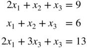
Solve the following system of equations using pivot operations:
- 3.4 It is proposed to build a reservoir of capacity x 1 to better control the supply of water to an irrigation district [16,17]. The inflow to the reservoir is expected to be 4.5 × 10⁶ acre–ft during the wet (rainy) season and 1.1 × 10⁶ acre–ft during the dry (summer) season. Between the reservoir and the irrigation district, one stream (A) adds water to and another stream (B) carries water away from the main stream, as shown in Figure 3.16. Stream A adds 1.2 × 10⁶ and 0.3 × 10⁶ acre–ft of water during the wet and dry seasons, respectively. Stream B takes away 0.5 × 10⁶ and 0.2 × 10⁶ acre–ft of water during the wet and dry seasons, respectively. Of the total amount of water released to the irrigation district per year (x 2), 30% is to be released during the wet season and 70% during the dry season. The yearly cost of diverting the required amount of water from the main stream to the irrigation district is given by 18(0.3x 2) + 12(0.7x 2). The cost of building and maintaining the reservoir, reduced to a yearly basis, is given by 25x 1. Determine the values of x 1 and x 2 to minimize the total yearly cost.
- 3.5
Solve the following system of equations using pivot operations:

- 3.6 What elementary operations can be used to transform
into
Find the solution of this system by reducing into canonical form.
- 3.7 Find the solution of the following LP problem graphically:
subject to
- 3.8 Find the solution of the following LP problem graphically:
subject to
- 3.9 Find the solution of the following LP problem graphically:
subject to
- 3.10 Find the solution of the following problem by the graphical method:

subject to
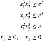
where e is the base of natural logarithms.
- 3.11 Prove Theorem 3.6.
For Problems 3.12–3.42, use a graphical procedure to identify (a) the feasible region, (b) the region where the slack (or surplus) variables are zero, and (c) the optimum solution.
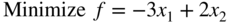
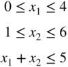
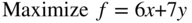
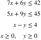
- 3.12
subject to
- 3.13 Rework Problem 12 when x and y are unrestricted in sign.
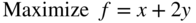
- 3.14

subject to

- 3.15 Rework Problem 14 when x and y are unrestricted in sign.
- 3.16
subject to
- 3.17 Rework Problem 16 by changing the objective to Minimize f = x − y.
- 3.18
subject to

- 3.19 Rework Problem 18 by changing the objective to Minimize f = x − y.
- 3.20
subject to


- 3.21
subject to

x and y are unrestricted in sign
- 3.22 Rework Problem 20 by changing the objective to Maximize f = x + y.
- 3.23
subject to

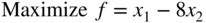
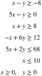
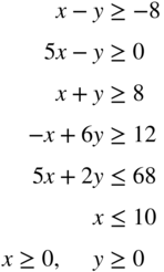
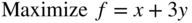
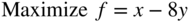
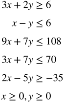
- 3.24
subject to


- 3.25 Rework Problem 24 by changing the objective to Maximize f = x − 8y.
- 3.26
subject to

x ≥ 0, y is unrestricted in sign
- 3.27
subject to

- 3.28
subject to
- 3.29
subject to

x ≥ 0, y is unrestricted in sign
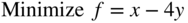
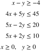
- 3.30
subject to

- 3.31 Rework Problem 30 by changing the objective to Maximize f = x − 4y.
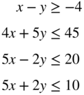
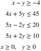
- 3.32
subject to


- 3.33 Rework Problem 32 by changing the objective to Maximize f = 4x + 5y.
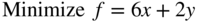
- 3.34 Rework Problem 32 by changing the objective to Minimize f = 6x + 2y.
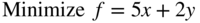
- 3.35
subject to

x and y are unrestricted in sign
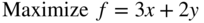
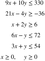
- 3.36
subject to

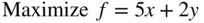
- 3.37 Rework Problem 36 by changing the objective to Maximize f = 5x + 2y.
- 3.38 Rework Problem 36 when x is unrestricted in sign and y ≥ 0.
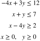
- 3.39
subject to

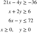
- 3.40
subject to
- 3.41 Rework Problem 40 by changing the constraint x + 2y ≥ 6 to x + 2y ≤ 6.
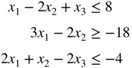
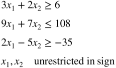
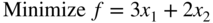
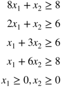
- 3.42
subject to


- 3.43
subject to

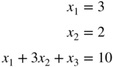
- 3.44 Reduce the system of equations

into a canonical system with x 1, x 2, and x 3 as basic variables. From this derive all other canonical forms.
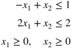
- 3.45
subject to


Find all the basic feasible solutions of the problem and identify the optimal solution.
- 3.46 A progressive university has decided to keep its library open round the clock and gathered that the following number of attendants are required to reshelve the books:
Time of day (h) Minimum number of attendants required 0–4 4 4–8 7 8–12 8 12–16 9 16–20 14 20–24 3 If each attendant works eight consecutive hours per day, formulate the problem of finding the minimum number of attendants necessary to satisfy the requirements above as a LP problem.
- 3.47 A paper mill received an order for the supply of paper rolls of widths and lengths as indicated below:
Number of rolls ordered Width of roll (m) Length (m) 1 6 100 1 8 300 1 9 200 The mill produces rolls only in two standard widths, 10 and 20 m. The mill cuts the standard rolls to size to meet the specifications of the orders. Assuming that there is no limit on the lengths of the standard rolls, find the cutting pattern that minimizes the trim losses while satisfying the order above.
- 3.48 Solve the LP problem stated in Example 1.6 for the following data: l = 2 m, W 1 = 3000 N, W 2 = 2000 N, W 3 = 1000 N, and w 1 = w 2 = w 3 = 200 N.
- 3.49 Find the solution of Problem 1.1 using the simplex method.
- 3.50 Find the solution of Problem 1.15 using the simplex method.
- 3.51 Find the solution of Example 3.1 using (a) the graphical method and (b) the simplex method.
- 3.52 In the scaffolding system shown in Figure 3.17, loads x 1 and x 2 are applied on beams 2 and 3, respectively. Ropes A and B can carry a load of W 1 = 300 lb. each; the middle ropes, C and D, can withstand a load of W 2 = 200 lb. each, and ropes E and F are capable of supporting a load W 3 = 100 lb. each. Formulate the problem of finding the loads x 1 and x 2 and their location parameters x 3 and x 4 to maximize the total load carried by the system, x 1 + x 2, by assuming that the beams and ropes are weightless.
- 3.53 A manufacturer produces three machine parts, A, B, and C. The raw material costs of parts A, B, and C are $5, $10, and $15 per unit, and the corresponding prices of the finished parts are $50, $75, and $100 per unit. Part A requires turning and drilling operations, while part B needs milling and drilling operations. Part C requires turning and milling operations. The number of parts that can be produced on various machines per day and the daily costs of running the machines are given below:
Machine part Number of parts that can be produced on Turning lathes Drilling machines Milling machines A 15 15 B 20 30 C 25 10 Cost of running the machines per day $250 $200 $300 Formulate the problem of maximizing the profit.
Solve Problems 3.54–3.90 by the simplex method.
- 3.54 Problem 1.22
- 3.55 Problem 1.23
- 3.56 Problem 1.24
- 3.57 Problem 1.25
- 3.58 Problem 7
- 3.59 Problem 12
- 3.60 Problem 13
- 3.61 Problem 14
- 3.62 Problem 15
- 3.63 Problem 16
- 3.64 Problem 17
- 3.65 Problem 18
- 3.66 Problem 19
- 3.67 Problem 20
- 3.68 Problem 21
- 3.69 Problem 22
- 3.70 Problem 23
- 3.71 Problem 24
- 3.72 Problem 25
- 3.73 Problem 26
- 3.74 Problem 27
- 3.75 Problem 28
- 3.76 Problem 29
- 3.77 Problem 30
- 3.78 Problem 31
- 3.79 Problem 32
- 3.80 Problem 33
- 3.81 Problem 34
- 3.82 Problem 35
- 3.83 Problem 36
- 3.84 Problem 37
- 3.85 Problem 38
- 3.86 Problem 39
- 3.87 Problem 40
- 3.88 Problem 41
- 3.89 Problem 42
- 3.90 Problem 43
- 3.91 (a) (b) The temperatures measured at various points inside a heated wall are given below:
Distance from the heated surface as a percentage of wall thickness, x i 0 20 40 60 80 100 Temperature, t i (°C) 400 350 250 175 100 50 It is decided to use a linear model to approximate the measured values as
(3.41)3.41
where t is the temperature, x the percentage of wall thickness, and a and b the coefficients that are to be estimated. Obtain the best estimates of a and b using linear programming with the following objectives.
- (a) Minimize the sum of absolute deviations between the measured values and those given by Eq. (3.41): ∑ i |a + bx i − t i |.
- (b) Minimize the maximum absolute deviation between the measured values and those given by Eq. (3.41):
- 3.92 A snack food manufacturer markets two kinds of mixed nuts, labeled A and B. Mixed nuts A contain 20% almonds, 10% cashew nuts, 15% walnuts, and 55% peanuts. Mixed nuts B contain 10% almonds, 20% cashew nuts, 25% walnuts, and 45% peanuts. A customer wants to use mixed nuts A and B to prepare a new mix that contains at least 4 lb. of almonds, 5 lb. of cashew nuts, and 6 lb. of walnuts, for a party. If mixed nuts A and B cost $2.50 and $3.00 per pound, respectively, determine the amounts of mixed nuts A and B to be used to prepare the new mix at a minimum cost.
- 3.93 A company produces three types of bearings, B
1, B
2, and B
3, on two machines, A
1 and A
2. The processing times of the bearings on the two machines are indicated in the following table:
Machine Processing time (min) for bearing: B 1 B 2 B 3 A 1 10 6 12 A 2 8 4 4 The times available on machines A 1 and A 2 per day are 1200 and 1000 minutes, respectively. The profits per unit of B 1, B 2, and B 3 are $4, $2, and $3, respectively. The maximum number of units the company can sell are 500, 400, and 600 for B 1, B 2, and B 3, respectively. Formulate and solve the problem for maximizing the profit.
- 3.94 Two types of printed circuit boards A and B are produced in a computer manufacturing company. The component placement time, soldering time, and inspection time required in producing each unit of A and B are given below:
Circuit board Time required per unit (min) for: Component placement Soldering Inspection A 16 10 4 B 10 12 8 If the amounts of time available per day for component placement, soldering, and inspection are 1500, 1000, and 500 person–minutes, respectively, determine the number of units of A and B to be produced for maximizing the production. If each unit of A and B contributes a profit of $10 and $15, respectively, determine the number of units of A and B to be produced for maximizing the profit.
- 3.95 A paper mill produces paper rolls in two standard widths; one with width 20 in. and the other with width 50 in. It is desired to produce new rolls with different widths as indicated below:
Width (in.) Number of rolls required 40 150 30 200 15 50 6 100 The new rolls are to be produced by cutting the rolls of standard widths to minimize the trim loss. Formulate the problem as an LP problem.
- 3.96 A manufacturer produces two types of machine parts, P
1 and P
2, using lathes and milling machines. The machining times required by each part on the lathe and the milling machine and the profit per unit of each part are given below:
Machine part Machine time (h) required by each unit on: Cost per unit Lathe Milling machine P 1 5 2 $200 P 2 4 4 $300 If the total machining times available in a week are 500 hours on lathes and 400 hours on milling machines, determine the number of units of P 1 and P 2 to be produced per week to maximize the profit.
- 3.97 A bank offers four different types of certificates of deposits (CDs) as indicated below:
CD type Duration (yr) Total interest at maturity (%) 1 0.5 5 2 1.0 7 3 2.0 10 4 4.0 15 If a customer wants to invest $50 000 in various types of CDs, determine the plan that yields the maximum return at the end of the fourth year.
- 98 The production of two machine parts A and B requires operations on a lathe (L), a shaper (S), a drilling machine (D), a milling machine (M), and a grinding machine (G). The machining times required by A and B on various machines are given below.
Machine part Machine time required (hours per unit) on: L S D M G A 0.6 0.4 0.1 0.5 0.2 B 0.9 0.1 0.2 0.3 0.3 The number of machines of different types available is given by L : 10, S : 3, D : 4, M : 6, and G : 5. Each machine can be used for eight hours a day for 30 days in a month.
- Determine the production plan for maximizing the output in a month
- If the number of units of A is to be equal to the number of units of B, find the optimum production plan.
- 3.99 A salesman sells two types of vacuum cleaners, A and B. He receives a commission of 20% on all sales, provided that at least 10 units each of A and B are sold per month. The salesman needs to make telephone calls to make appointments with customers and demonstrate the products in order to sell the products. The selling price of the products, the average money to be spent on telephone calls, the time to be spent on demonstrations, and the probability of a potential customer buying the product are given below:
Vacuum cleaner Selling price per unit Money to be spent on telephone calls to find a potential customer Time to be spent in demonstrations to a potential customer (h) Probability of a potential customer buying the product A $250 $3 3 0.4 B $100 $1 1 0.8 In a particular month, the salesman expects to sell at most 25 units of A and 45 units of B. If he plans to spend a maximum of 200 hours in the month, formulate the problem of determining the number of units of A and B to be sold to maximize his income.
- 3.100 An electric utility company operates two thermal power plants, A and B, using three different grades of coal, C
1, C
2, and C
3. The minimum power to be generated at plants A and B is 30 and 80 MWh, respectively. The quantities of various grades of coal required to generate 1 MWh of power at each power plant, the pollution caused by the various grades of coal at each power plant, and the costs of coal are given in the following table:
Coal type Quantity of coal required to generate 1 MWh at the power plant (tons) Pollution caused at power plant Cost of coal at power plant A B A B A B C 1 2.5 1.5 1.0 1.5 20 18 C 2 1.0 2.0 1.5 2.0 25 28 C 3 3.0 2.5 2.0 2.5 18 12 Formulate the problem of determining the amounts of different grades of coal to be used at each power plant to minimize (a) the total pollution level, and (b) the total cost of operation.
- 3.101 A grocery store wants to buy five different types of vegetables from four farms in a month. The prices of the vegetables at different farms, the capacities of the farms, and the minimum requirements of the grocery store are indicated in the following table:
Price ($/ton) of vegetable type Farm 1 (Potato) 2 (Tomato) 3 (Okra) 4 (Eggplant) 5 (Spinach) Maximum (of all types combined) they can supply 1 200 600 1600 800 1200 180 2 300 550 1400 850 1100 200 3 250 650 1500 700 1000 100 4 150 500 1700 900 1300 120 Minimum amount required (tons) 100 60 20 80 40 Formulate the problem of determining the buying scheme that corresponds to a minimum cost.
- 3.102 A steel plant produces steel using four different types of processes. The iron ore, coal, and labor required, the amounts of steel and side products produced, the cost information, and the physical limitations on the system are given below:
Process type Iron ore required (tons/day) Coal required (tons/day) Labor required (person‐days) Steel produced (tons/day) Side products produced (tons/day) 1 5 3 6 4 1 2 8 5 12 6 2 3 3 2 5 2 1 4 10 7 12 6 4 Cost $50/ton $10/ton $150/ person‐day $350/ton $100/ton Limitations 600 tons available per month 250 tons available per month No limitations on availability of labor All steel produced can be sold Only 200 tons can be sold per month Assuming that a particular process can be employed for any number of days in a 30‐day month, determine the operating schedule of the plant for maximizing the profit.
- 3.103 Solve 3.7 using MATLAB (simplex method).
- 3.104 Solve Problem 12 using MATLAB (simplex method).
- 3.105 Solve Problem 24 using MATLAB (simplex method).
- 3.106 Find the optimal solution of the LP problem stated in Problem 45 using MATLAB (simplex method).
- 3.107 Find the optimal solution of the LP problem described in Problem 101 using MATLAB.