
4
Linear Programming II: Additional Topics and Extensions
4.1 Introduction
If a Linear Programming (LP) problem involving several variables and constraints is to be solved by using the simplex method described in Chapter 3, it requires a large amount of computer storage and time. Some techniques, which require less computational time and storage space compared to the original simplex method, have been developed. Among these techniques, the revised simplex method is very popular. The principal difference between the original simplex method and the revised one is that in the former we transform all the elements of the simplex table, while in the latter we need to transform only the elements of an inverse matrix. Associated with every LP problem, another LP problem, called the dual, can be formulated. The solution of a given LP problem, in many cases, can be obtained by solving its dual in a much simpler manner.
As stated above, one of the difficulties in certain practical LP problems is that the number of variables and/or the number of constraints is so large that it exceeds the storage capacity of the available computer. If the LP problem has a special structure, a principle known as the decomposition principle can be used to solve the problem more efficiently. In many practical problems, one will be interested not only in finding the optimum solution to a LP problem, but also in finding how the optimum solution changes when some parameters of the problem, such as cost coefficients change. Hence, the sensitivity or postoptimality analysis becomes very important.
An important special class of LP problems, known as transportation problems, occurs often in practice. These problems can be solved by algorithms that are more efficient (for this class of problems) than the simplex method. Karmarkar's method is an interior method and has been shown to be superior to the simplex method of Dantzig for large problems. The quadratic programming problem is the best‐behaved nonlinear programming problem. It has a quadratic objective function and linear constraints and is convex (for minimization problems). Hence the quadratic programming problem can be solved by suitably modifying the linear programming techniques. All these topics are discussed in this chapter.
4.2 Revised Simplex Method
We notice that the simplex method requires the computing and recording of an entirely new tableau at each iteration. But much of the information contained in the table is not used; only the following items are needed.
- The relative cost coefficients
 to compute1
(4.1)
to compute1
(4.1)
 determines the variable x
s
that has to be brought into the basis in the next iteration.
determines the variable x
s
that has to be brought into the basis in the next iteration. - By assuming that
 < 0, the elements of the updated column

and the values of the basic variables

have to be calculated. With this information, the variable x r that has to be removed from the basis is found by computing the quantity
(4.2)
and a pivot operation is performed on
 . Thus, only one nonbasic column
  of the current tableau is useful in finding x
r
. Since most of the linear programming problems involve many more variables (columns) than constraints (rows), considerable effort and storage is wasted in dealing with the
of the current tableau is useful in finding x
r
. Since most of the linear programming problems involve many more variables (columns) than constraints (rows), considerable effort and storage is wasted in dealing with the  for j ≠ s. Hence, it would be more efficient if we can generate the modified cost coefficients
  and the column
  , from the original problem data itself. The revised simplex method is used for this purpose; it makes use of the inverse of the current basis matrix in generating the required quantities.
Theoretical Development. Although the revised simplex method is applicable for both phase I and phase II computations, the method is initially developed by considering linear programming in phase II for simplicity. Later, a step‐by‐step procedure is given to solve the general linear programming problem involving both phases I and II.
Let the given linear programming problem (phase II) be written in column form as
Minimize
subject to
where the jth column of the coefficient matrix A is given by
Assuming that the linear programming problem has a solution, let
be a basis matrix with

representing the corresponding vectors of basic variables and cost coefficients, respectively. If X B is feasible, we have
As in the regular simplex method, the objective function is included as the (m + 1)th equation and −f is treated as a permanent basic variable. The augmented system can be written as

where

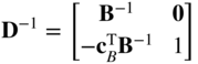
Since B is a feasible basis for the system of Eq (4.4), the matrix D defined by

will be a feasible basis for the augmented system of Eq (4.6). The inverse of D can be found to be
Definition. The row vector
is called the vector of simplex multipliers relative to the f equation. If the computations correspond to phase I, two vectors of simplex multipliers, one relative to the f equation, and the other relative to the w equation are to be defined as

By premultiplying each column of Eq. (4.6) by D −1, we obtain the following canonical system of equations 2:

where

From Eq. (4.8), the updated column ![]() can be identified as
can be identified as
and the modified cost coefficient ![]() as
as
Equations (4.9) and (4.10) can be used to perform a simplex iteration by generating ![]() and
and ![]() from the original problem data, A
j
and c
j
.
from the original problem data, A
j
and c
j
.
Once ![]() and
and ![]() are computed, the pivot element
are computed, the pivot element ![]() can be identified by using Eqs. (4.1) and (4.2). In the next step, P
s
is introduced into the basis and P
jr
is removed. This amounts to generating the inverse of the new basis matrix. The computational procedure can be seen by considering the matrix:
can be identified by using Eqs. (4.1) and (4.2). In the next step, P
s
is introduced into the basis and P
jr
is removed. This amounts to generating the inverse of the new basis matrix. The computational procedure can be seen by considering the matrix:

where e i is a (m + 1)‐dimensional unit vector with a one in the ith row. Premultiplication of the above matrix by D −1 yields

By carrying out a pivot operation on ![]() , this matrix transforms to
, this matrix transforms to
where all the elements of the vector
β
are, in general, nonzero and the second partition gives the desired matrix ![]() .3 It can be seen that the first partition (matrix I) is included only to illustrate the transformation, and it can be dropped in actual computations. Thus, in practice, we write the m + 1 × m + 2 matrix
.3 It can be seen that the first partition (matrix I) is included only to illustrate the transformation, and it can be dropped in actual computations. Thus, in practice, we write the m + 1 × m + 2 matrix

and carry out a pivot operation on ![]() . The first m + 1 columns of the resulting matrix will give us the desired matrix
. The first m + 1 columns of the resulting matrix will give us the desired matrix ![]() .
.
Procedure. The detailed iterative procedure of the revised simplex method to solve a general linear programming problem is given by the following steps.
- Write the given system of equations in canonical form, by adding the artificial variables x
n+1
, x
n+2
, …, x
n+m
, and the infeasibility form for phase I as shown below:
(4.14)
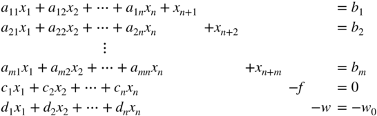
Here the constants b i , i = 1 to m, are made nonnegative by changing, if necessary, the signs of all terms in the original equations before the addition of the artificial variables x n+i , i = 1 to m. Since the original infeasibility form is given by
(4.15)
the artificial variables can be eliminated from Eq. (4.15) by adding the first m equations of Eq. (4.14) and subtracting the result from Eq. (4.15). The resulting equation is shown as the last equation in Eq. (4.14) with
(4.16)
Equations (4.14) are written in tableau form as shown in Table 4.1.
- The iterative procedure (cycle 0) is started with x
n+1
, x
n+2
, …, x
n+m
, −f, and −w as the basic variables. A table is opened by entering the coefficients of the basic variables and the constant terms as shown in Table 4.2. The starting basis matrix is, from Table 4.1, B = I, and its inverse B
−1 = [β
ij
] can also be seen to be an identity matrix in Table 4.2. The rows corresponding to −f and −w in Table 4.2 give the negative of simplex multipliers π
i
and σ
i
(i = 1 to m), respectively. These are also zero since c
B
= d
B
= 0 and hence
In general, at the start of some cycle k (k = 0 to start with) we open a table similar to Table 4.2, as shown in Table 4.4. This can also be interpreted as composed of the inverse of the current basis, B −1 = [β ij ], two rows for the simplex multipliers π i and σ i , a column for the values of the basic variables in the basic solution, and a column for the variable x s . At the start of any cycle, all entries in the table, except the last column, are known.
- The values of the relative cost factors
 (for phase I) or
  (for phase II) are computed as

and entered in a table form as shown in Table 4.3. For cycle 0, σ T = 0 and hence
 ≡ d
j
.
≡ d
j
. - If the current cycle corresponds to phase I, find whether all
 . If all
  and
and  , there is no feasible solution to the linear programming problem, so the process is terminated. If all
  and
and  , the current basic solution is a basic feasible solution to the linear programming problem and hence phase II is started by (i) dropping all variables x
j
with
, the current basic solution is a basic feasible solution to the linear programming problem and hence phase II is started by (i) dropping all variables x
j
with  , (ii) dropping the w row of the tableau, and (iii) restarting the cycle (step 3) using phase II rules.
If some
 , choose x
s
as the variable to enter the basis in the next cycle in place of the present rth basic variable (r will be determined later) such that
, choose x
s
as the variable to enter the basis in the next cycle in place of the present rth basic variable (r will be determined later) such that
On the other hand, if the current cycle corresponds to phase II, find whether all
 . If all
  , the current basic feasible solution is also an optimal solution and hence terminate the process. If some
  , choose x
s
to enter the basic set in the next cycle in place of the rth basic variable (r to be found later), such that
, choose x
s
to enter the basic set in the next cycle in place of the rth basic variable (r to be found later), such that
- Compute the elements of the x
s
column from Eq. (4.9) as

that is,
and enter in the last column of Table 4.2 (if cycle 0) or Table 4.4 (if cycle k).
- Inspect the signs of all entries
 , i = 1 to m. If all
  , the class of solutions
 if x
ji
is a basic variable, and x
j
= 0 if x
j
is a nonbasic variable (j ≠ s), satisfies the original system and has the property
if x
ji
is a basic variable, and x
j
= 0 if x
j
is a nonbasic variable (j ≠ s), satisfies the original system and has the property
Hence terminate the process. On the other hand, if some
 , select the variable x
r
that can be dropped in the next cycle as
, select the variable x
r
that can be dropped in the next cycle as
In the case of a tie, choose r at random.
- To bring x
s
into the basis in place of x
r
, carry out a pivot operation on the element
 in Table 4.4 and enter the result as shown in Table 4.5. As usual, the last column of Table 4.5 will be left blank at the beginning of the current cycle k + 1. Also, retain the list of basic variables in the first column of Table 4.5 the same as in Table 4.4, except that j
r
is changed to the value of s determined in step 4.
in Table 4.4 and enter the result as shown in Table 4.5. As usual, the last column of Table 4.5 will be left blank at the beginning of the current cycle k + 1. Also, retain the list of basic variables in the first column of Table 4.5 the same as in Table 4.4, except that j
r
is changed to the value of s determined in step 4. - Go to step 3 to initiate the next cycle, k + 1.
Table 4.1 Original System of Equations.
| Admissible (original) variable | Artificial variable | Objective variable | |||||||
| x 1 | x 2 | ⋯x j | ⋯x n | x n+1 | x n+2 ⋯ | x n+m | −f | −w | Constant |
| Initial basis | |||||||||
| 1 | b 1 | ||||||||
| 1 | b 2 | ||||||||

|

|
|
|
||||||
| 1 | b m | ||||||||
| c 1 | c 2 | c j | c n | 0 | 0 | 0 | 1 | 0 | 0 |
| d 1 | d 2 | d j | d n | 0 | 0 | 0 | 0 | 1 | −w 0 |
Table 4.2 Table at the Beginning of Cycle 0.
| Columns of the canonical form | ||||||||||
| Basic variables | x n+1 | x n+2 | ⋯ | x n+r | ⋯ | x n+m | −f | −w | Value of the basic variable | x s a |
| x n+1 | 1 | b 1 | ||||||||
| x n+2 | 1 | b 2 | ||||||||
| ⋮ | ⋮ | |||||||||
| x n+r | 1 | b r | ||||||||
| ⋮ | ⋮ | |||||||||
| x n+m | 1 | b m | ||||||||
| Inverse of the basis | ||||||||||
| −f | 0 | 0 | ⋯ | 0 | ⋯ | 0 | 1 | 0 | ||
| −w | 0 | 0 | ⋯ | 0 | ⋯ | 0 | 1 |
|
||
a This column is blank at the beginning of cycle 0 and filled up only at the end of cycle 0.
Table 4.3
Relative Cost Factor ![]() or
or ![]() .
.
| Variable x j | ||||||||
| Cycle number | x 1 | x 2 | ⋯ | xn | x n+1 | x n+2 | ⋯ | x n+m |
|
||||||||
| d 1 | d 2 | ⋯ | d n | 0 | 0 | ⋯ | 0 | |
| Use the values of σ i (if phase I) or π i (if phase II) of the current cycle and compute | ||||||||
|
|
||||||||
| or | ||||||||

|
||||||||
|
|
||||||||
|
Enter |
||||||||
Table 4.4 Table at the Beginning of Cycle k.
| Columns of the original canonical form | |||||
| Basic variable | x n+1 ⋯ x n+m | −f | −w | Value of the basic variable | xs a |
|
[β
ij
] = [ |
|||||
| ← Inverse of the basis → | |||||
| x j1 | β 11 ⋯ β 1m |
|
|
||
| ⋮ | ⋮ ⋮ | ⋮ | |||
| x jr | β r1 ⋯ β rm |
|
|
||
| ⋮ | ⋮ ⋮ | ⋮ | |||
| x jm | β m1 ⋯ β mm |
|
|
||
| −f | −π 1 ⋯ −π m | 1 |
|

|
|
|
(−π
j
= + |
|||||
|
|
−σ 1 ⋯ −σ m | 1 |
|
|
|
|
(−σ
j
= + |
|||||
a This column is blank at the start of cycle k and is filled up only at the end of cycle k.
4.3 Duality in Linear Programming
Associated with every linear programming problem, called the primal, there is another linear programming problem called its dual. These two problems possess very interesting and closely related properties. If the optimal solution to any one is known, the optimal solution to the other can readily be obtained. In fact, it is immaterial which problem is designated the primal since the dual of a dual is the primal. Because of these properties, the solution of a linear programming problem can be obtained by solving either the primal or the dual, whichever is easier. This section deals with the primal–dual relations and their application in solving a given linear programming problem.
4.3.1 Symmetric Primal–Dual Relations
A nearly symmetric relation between a primal problem and its dual problem can be seen by considering the following system of linear inequalities (rather than equations).
Primal Problem

Dual Problem. As a definition, the dual problem can be formulated by transposing the rows and columns of Eq. (4.17) including the right‐hand side and the objective function, reversing the inequalities and maximizing instead of minimizing. Thus, by denoting the dual variables as y 1 , y 2 , …, y m , the dual problem becomes

Equations (4.17) and (4.18) are called symmetric primal–dual pairs and it is easy to see from these relations that the dual of the dual is the primal.
4.3.2 General Primal–Dual Relations
Although the primal–dual relations of Section 4.3.1 are derived by considering a system of inequalities in nonnegative variables, it is always possible to obtain the primal–dual relations for a general system consisting of a mixture of equations, less than or greater than type of inequalities, nonnegative variables or variables unrestricted in sign by reducing the system to an equivalent inequality system of Eq. (4.17). The correspondence rules that are to be applied in deriving the general primal–dual relations are given in Table 4.11 and the primal–dual relations are shown in Table 4.12.
Table 4.11 Correspondence Rules for Primal–Dual Relations.
| Primal quantity | Corresponding dual quantity |
| Objective function: Minimize c T X | Maximize Y T b |
| Variable x i ≥ 0 | ith constraint Y T A i ≤ c i (inequality) |
| Variable x i unrestricted in sign | ith constraint Y T A i = c i (equality) |
| jth constraint, A j X = b j (equality) | jth variable y j unrestricted in sign |
| jth constraint, A j X ≥ b j (inequality) | jth variable y j ≥ 0 |
| Coefficient matrix A ≡ [A 1 … A m ] | Coefficient matrix A T ≡ [A 1 , …, A m ]T |
| Right‐hand‐side vector b | Right‐hand‐side vector c |
| Cost coefficients c | Cost coefficients b |
Table 4.12 Primal–Dual Relations.
| Primal problem | Corresponding dual problem |
|

|

|

|
| where | where |
| x i ≥ 0, i = 1, 2, …, n *; | y i ≥ 0, i = m * + 1, m * + 2, …, m; |
| and | and |
| x i unrestricted in sign, i = n * + 1, n * + 2, …, n | y i unrestricted in sign, i = 1, 2, …, m * |
4.3.3 Primal–Dual Relations when the Primal Is in Standard Form
If m * = m and n * = n, primal problem shown in Table 4.12 reduces to the standard form and the general primal–dual relations take the special form shown in Table 4.13. It is to be noted that the symmetric primal–dual relations, discussed in Section 4.3.1, can also be obtained as a special case of the general relations by setting m * = 0 and n * = n in the relations of Table 4.12.
Table 4.13 Primal–Dual Relations Where m * = m and n * = n.
| Primal problem | Corresponding dual problem |
Minimize 
|
Maximize 
|
| subject to | subject to |
|
|
| where | where |
| x i ≥ 0, i = 1, 2, …, n | y i is unrestricted in sign, i = 1, 2,⋯, m |
| In matrix form | In matrix form |
| Minimize f = c T X | Maximize ν = Y T b |
| subject to | subject to |
| AX = b | A T Y ≤ c |
| where | where |
| X ≥ 0 | Y is unrestricted in sign |
4.3.4 Duality Theorems
The following theorems are useful in developing a method for solving LP problems using dual relationships. The proofs of these theorems can be found in Ref. [10].
4.3.5 Dual Simplex Method
There exist a number of situations in which it is required to find the solution of a linear programming problem for a number of different right‐hand‐side vectors b (i). Similarly, in some cases, we may be interested in adding some more constraints to a linear programming problem for which the optimal solution is already known. When the problem has to be solved for different vectors b (i), one can always find the desired solution by applying the two phases of the simplex method separately for each vector b (i). However, this procedure will be inefficient since the vectors b (i) often do not differ greatly from one another. Hence the solution for one vector, say, b (1) may be close to the solution for some other vector, say, b (2). Thus a better strategy is to solve the linear programming problem for b (1) and obtain an optimal basis matrix B. If this basis happens to be feasible for all the right‐hand‐side vectors, that is, if
then it will be optimal for all cases. On the other hand, if the basis B is not feasible for some of the right‐hand‐side vectors, that is, if
then the vector of simplex multipliers
will form a dual feasible solution since the quantities
are independent of the right‐hand‐side vector b (r). A similar situation exists when the problem has to be solved with additional constraints.
In both the situations discussed above, we have an infeasible basic (primal) solution whose associated dual solution is feasible. Several methods have been proposed, as variants of the regular simplex method, to solve a linear programming problem by starting from an infeasible solution to the primal. All these methods work in an iterative manner such that they force the solution to become feasible as well as optimal simultaneously at some stage. Among all the methods, the dual simplex method developed by Lemke [2] and the primal–dual method developed by Dantzig et al. [3] have been most widely used. Both these methods have the following important characteristics:
- They do not require the phase I computations of the simplex method. This is a desirable feature since the starting point found by phase I may be nowhere near optimal, since the objective of phase I ignores the optimality of the problem completely.
- Since they work toward feasibility and optimality simultaneously, we can expect to obtain the solution in a smaller total number of iterations.
We shall consider only the dual simplex algorithm in this section.
Algorithm. As stated earlier, the dual simplex method requires the availability of a dual feasible solution that is not primal feasible to start with. It is the same as the simplex method applied to the dual problem but is developed such that it can make use of the same tableau as the primal method. Computationally, the dual simplex algorithm also involves a sequence of pivot operations, but with different rules (compared to the regular simplex method) for choosing the pivot element.
Let the problem to be solved be initially in canonical form with some of the ![]() , the relative cost coefficients corresponding to the basic variables c
j
= 0, and all other c
j
≥ 0. Since some of the
, the relative cost coefficients corresponding to the basic variables c
j
= 0, and all other c
j
≥ 0. Since some of the ![]() are negative, the primal solution will be infeasible, and since all
are negative, the primal solution will be infeasible, and since all ![]() , the corresponding dual solution will be feasible. Then the simplex method works according to the following iterative steps.
, the corresponding dual solution will be feasible. Then the simplex method works according to the following iterative steps.
- Select row r as the pivot row such that
(4.22)
- Select column s as the pivot column such that
(4.23)

If all
 ≥ 0, the primal will not have any feasible (optimal) solution.
 - Carry out a pivot operation on

- Test for optimality: If all
 ≥ 0, the current solution is optimal and hence stop the iterative procedure. Otherwise, go to step 1.
Remarks:
- Since we are applying the simplex method to the dual, the dual solution will always be maintained feasible, and hence all the relative cost factors of the primal
 will be nonnegative. Thus, the optimality test in step 4 is valid because it guarantees that all
  are also nonnegative, thereby ensuring a feasible solution to the primal.
 - We can see that the primal will not have a feasible solution when all a
rj
are nonnegative from the following reasoning. Let (x
1
, x
2
, …, x
m
) be the set of basic variables. Then the rth basic variable, x
r
, can be expressed as
It can be seen that if
 < 0 and
  ≥ 0 for all j, x
r
cannot be made nonnegative for any nonnegative value of x
j
. Thus, the primal problem contains an equation (the rth one) that cannot be satisfied by any set of nonnegative variables and hence will not have any feasible solution.
≥ 0 for all j, x
r
cannot be made nonnegative for any nonnegative value of x
j
. Thus, the primal problem contains an equation (the rth one) that cannot be satisfied by any set of nonnegative variables and hence will not have any feasible solution.
The following example is considered to illustrate the dual simplex method.
4.4 Decomposition Principle
Some of the linear programming problems encountered in practice may be very large in terms of the number of variables and/or constraints. If the problem has some special structure, it is possible to obtain the solution by applying the decomposition principle developed by Dantzing and Wolfe [4]. In the decomposition method, the original problem is decomposed into small subproblems and then these subproblems are solved almost independently. The procedure, when applicable, has the advantage of making it possible to solve large‐scale problems that may otherwise be computationally very difficult or infeasible. As an example of a problem for which the decomposition principle can be applied, consider a company having two factories, producing three and two products, respectively. Each factory has its own internal resources for production, namely, workers and machines. The two factories are coupled by the fact that there is a shared resource that both use, for example, a raw material whose availability is limited. Let b 2 and b 3 be the maximum available internal resources for factory 1, and let b 4 and b 5 be the similar availabilities for factory 2. If the limitation on the common resource is b 1, the problem can be stated as follows:
subject to

where x i and y j are the quantities of the various products produced by the two factories (design variables) and the a ij are the quantities of resource i required to produce 1 unit of product j.
An important characteristic of the problem stated in Eq. (4.24) is that its constraints consist of two independent sets of inequalities. The first set consists of a coupling constraint involving all the design variables, and the second set consists of two groups of constraints, each group containing the design variables of that group only. This problem can be generalized as follows:
subject to

where

It can be noted that if the size of the matrix A
k
is (r
0 × m
k
) and that of B
k
is (r
k
× m
k
), the problem has ![]() constraints and
constraints and ![]() variables.
variables.
Since there are a large number of constraints in the problem stated in Eq. (4.25), it may not be computationally efficient to solve it by using the regular simplex method. However, the decomposition principle can be used to solve it in an efficient manner. The basic solution procedure using the decomposition principle is given by the following steps.
- Define p subsidiary constraint sets using Eq. (4.25) as
(4.26)
The subsidiary constraint set
(4.27)
represents r k equality constraints. These constraints along with the requirement X k ≥ 0 define the set of feasible solutions of Eq. (4.27). Assuming that this set of feasible solutions is a bounded convex set, let s k be the number of vertices of this set. By using the definition of convex combination of a set of points,4 any point X k satisfying Eq. (4.27) can be represented as
(4.28) (4.29)
 (4.30)
where
 are the extreme points of the feasible set defined by Eq. (4.27). These extreme points
  , can be found by solving the Eq. (4.27).
 - These new Eq. (4.28) imply the complete solution space enclosed by the constraints
(4.31)

By substituting Eq. (4.28) into Eq. (4.25), it is possible to eliminate the subsidiary constraint sets from the original problem and obtain the following equivalent form:
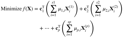
subject to
 (4.32)
Since the extreme points
 are known from the solution of the set B
k
X
k
= b
k
,
X
k
≥ 0
, k = 1, 2, …, p, and since c
k
and A
k
, k = 1, 2, …, p, are known as problem data, the unknowns in Eq. (4.32) are μ
j,i
, i = 1, 2, …, s
j
; j = 1, 2, …, p. Hence μ
j,i
will be the new decision variables of the modified problem stated in Eq. (4.32).
are known from the solution of the set B
k
X
k
= b
k
,
X
k
≥ 0
, k = 1, 2, …, p, and since c
k
and A
k
, k = 1, 2, …, p, are known as problem data, the unknowns in Eq. (4.32) are μ
j,i
, i = 1, 2, …, s
j
; j = 1, 2, …, p. Hence μ
j,i
will be the new decision variables of the modified problem stated in Eq. (4.32). - Solve the linear programming problem stated in Eq. (4.32) by any of the known techniques and find the optimal values of μ
j,i
. Once the optimal values
 are determined, the optimal solution of the original problem can be obtained as
where

Remarks:
- It is to be noted that the new problem in Eq. (4.32) has (r
0 + p) equality constraints only as against
 in the original problem of Eq. (4.25). Thus, there is a substantial reduction in the number of constraints due to the application of the decomposition principle. At the same time, the number of variables might increase from
  , depending on the number of extreme points of the different subsidiary problems defined by Eq. (4.31). The modified problem, however, is computationally more attractive since the computational effort required for solving any linear programming problem depends primarily on the number of constraints rather than on the number of variables.
 - The procedure outlined above requires the determination of all the extreme points of every subsidiary constraint set defined by Eq. (4.31) before the optimal values
 are found. However, this is not necessary when the revised simplex method is used to implement the decomposition algorithm [5].
 - If the size of the problem is small, it will be convenient to enumerate all the extreme points of the subproblems and use the simplex method to solve the problem. This procedure is illustrated in the following example.
4.5 Sensitivity or Postoptimality Analysis
In most practical problems, we are interested not only in optimal solution of the LP problem, but also in how the solution changes when the parameters of the problem change. The change in the parameters may be discrete or continuous. The study of the effect of discrete parameter changes on the optimal solution is called sensitivity analysis and that of the continuous changes is termed parametric programming. One way to determine the effects of changes in the parameters is to solve a series of new problems once for each of the changes made. This is, however, very inefficient from a computational point of view. Some techniques that take advantage of the properties of the simplex solution are developed to make a sensitivity analysis. We study some of these techniques in this section. There are five basic types of parameter changes that affect the optimal solution:
- Changes in the right‐hand‐side constants b i
- Changes in the cost coefficients c j
- Changes in the coefficients of the constraints a ij
- Addition of new variables
- Addition of new constraints
In general, when a parameter is changed, it results in one of three cases:
- The optimal solution remains unchanged; that is, the basic variables and their values remain unchanged.
- The basic variables remain the same, but their values are changed.
- The basic variables as well as their values are changed.
4.5.1 Changes in the Right‐Hand‐Side Constants bi
Suppose that we have found the optimal solution to a LP problem. Let us now change the b
i
to b
i
+ Δb
i
so that the new problem differs from the original only on the right‐hand side. Our interest is to investigate the effect of changing b
i
to b
i
+ Δb
i
on the original optimum. We know that a basis is optimal if the relative cost coefficients corresponding to the nonbasic variables ![]() are nonnegative. By considering the procedure according to which
are nonnegative. By considering the procedure according to which ![]() are obtained, we can see that the values of
are obtained, we can see that the values of ![]() are not related to the b
i
. The values of
are not related to the b
i
. The values of ![]() depend only on the basis, on the coefficients of the constraint matrix, and the original coefficients of the objective function. The relation is given in Eq. (4.10):
depend only on the basis, on the coefficients of the constraint matrix, and the original coefficients of the objective function. The relation is given in Eq. (4.10):
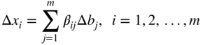
Thus, changes in b i will affect the values of basic variables in the optimal solution and the optimality of the basis will not be affected provided that the changes made in b i do not make the basic solution infeasible. Thus, if the new basic solution remains feasible for the new right‐hand side, that is, if
then the original optimal basis, B, also remains optimal for the new problem. Since the original solution, say5

is given by
Equation (4.34) can also be expressed as
where
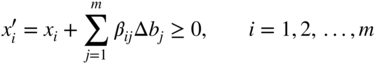
Hence the original optimal basis B remains optimal provided that the changes made in b i , Δb i , satisfy the inequalities (4.36). The change in the value of the ith optimal basic variable, Δx i , due to the change in b i is given by
that is,
Finally, the change in the optimal value of the objective function (Δf) due to the change Δb i can be obtained as

Suppose that the changes made in b i (Δb i ) are such that the inequality (4.34) is violated for some variables so that these variables become infeasible for the new right‐hand‐side vector. Our interest in this case will be to determine the new optimal solution. This can be done without reworking the problem from the beginning by proceeding according to the following steps:
- Replace the
 of the original optimal tableau by the new values,
  and change the signs of all the numbers that are lying in the rows in which the infeasible variables appear, that is, in rows for which
- Add artificial variables to these rows, thereby replacing the infeasible variables in the basis by the artificial variables.
- Go through the phase I calculations to find a basic feasible solution for the problem with the new right‐hand side.
- If the solution found at the end of phase I is not optimal, we go through the phase II calculations to find the new optimal solution.
The procedure outlined above saves considerable time and effort compared to the reworking of the problem from the beginning if only a few variables become infeasible with the new right‐hand side. However, if the number of variables that become infeasible are not few, the procedure above might also require as much effort as the one involved in reworking of the problem from the beginning.
4.5.2 Changes in the Cost Coefficients cj
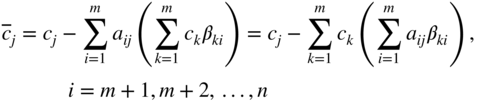
The problem here is to find the effect of changing the cost coefficients from c j to c j + Δc j on the optimal solution obtained with c j . The relative cost coefficients corresponding to the nonbasic variables, x m+1, x m+2 , …, x n are given by Eq. (4.10):
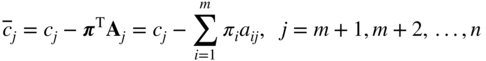
where the simplex multipliers π i are related to the cost coefficients of the basic variables by the relation
that is,
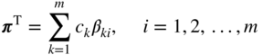
From Eqs. (4.40) and (4.41), we obtain
If the c
j
are changed to c
j
+ Δc
j
, the original optimal solution remains optimal, provided that the new values of ![]() ,
, ![]() satisfy the relation
satisfy the relation
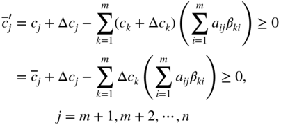
where ![]() indicate the values of the relative cost coefficients corresponding to the original optimal solution.
indicate the values of the relative cost coefficients corresponding to the original optimal solution.
In particular, if changes are made only in the cost coefficients of the nonbasic variables, Eq. (4.43) reduces to
If Eq. (4.43) is satisfied, the changes made in c j , Δc j , will not affect the optimal basis and the values of the basic variables. The only change that occurs is in the optimal value of the objective function according to
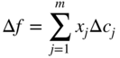
and this change will be zero if only the c j of nonbasic variables are changed.
Suppose that Eq. (4.43) is violated for some of the nonbasic variables. Then it is possible to improve the value of the objective function by bringing any nonbasic variable that violates Eq. (4.43) into the basis provided that it can be assigned a nonzero value. This can be done easily with the help of the previous optimal table. Since some of the ![]() are negative, we start the optimization procedure again by using the old optimum as an initial feasible solution. We continue the iterative process until the new optimum is found. As in the case of changing the right‐hand‐side b
i
, the effectiveness of this procedure depends on the number of violations made in Eq. (4.43) by the new values c
j
+ Δc
j
.
are negative, we start the optimization procedure again by using the old optimum as an initial feasible solution. We continue the iterative process until the new optimum is found. As in the case of changing the right‐hand‐side b
i
, the effectiveness of this procedure depends on the number of violations made in Eq. (4.43) by the new values c
j
+ Δc
j
.
In some of the practical problems, it may become necessary to solve the optimization problem with a series of objective functions. This can be accomplished without reworking the entire problem for each new objective function. Assume that the optimum solution for the first objective function is found by the regular procedure. Then consider the second objective function as obtained by changing the first one and evaluate Eq. (4.43). If the resulting ![]() ≥ 0, the old optimum still remains as optimum and one can proceed to the next objective function in the same manner. On the other hand, if one or more of the resulting
≥ 0, the old optimum still remains as optimum and one can proceed to the next objective function in the same manner. On the other hand, if one or more of the resulting ![]() < 0, we can adopt the procedure outlined above and continue the iterative process using the old optimum as the starting feasible solution. After the optimum is found, we switch to the next objective function.
< 0, we can adopt the procedure outlined above and continue the iterative process using the old optimum as the starting feasible solution. After the optimum is found, we switch to the next objective function.
4.5.3 Addition of New Variables
Suppose that the optimum solution of a LP problem with n variables x 1 , x 2 , …, x n has been found and we want to examine the effect of adding some more variables x n+k , k = 1, 2, …, on the optimum solution. Let the constraint coefficients and the cost coefficients corresponding to the new variables x n+k be denoted by a i, n+k , i = 1 to m and c n+k , respectively. If the new variables are treated as additional nonbasic variables in the old optimum solution, the corresponding relative cost coefficients are given by
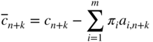
where π
1
, π
2
, …, π
m
are the simplex multipliers corresponding to the original optimum solution. The original optimum remains optimum for the new problem also provided that ![]() ≥ 0 for all k. However, if one or more
≥ 0 for all k. However, if one or more ![]() < 0, it pays to bring some of the new variables into the basis, provided that they can be assigned a nonzero value. For bringing a new variable into the basis, we first have to transform the coefficients a
i,n+k
into
< 0, it pays to bring some of the new variables into the basis, provided that they can be assigned a nonzero value. For bringing a new variable into the basis, we first have to transform the coefficients a
i,n+k
into ![]() ,
n+k
so that the columns of the new variables correspond to the canonical form of the old optimal basis. This can be done by using Eq. (4.9) as
,
n+k
so that the columns of the new variables correspond to the canonical form of the old optimal basis. This can be done by using Eq. (4.9) as
that is,
where B −1 = [β ij ] is the inverse of the old optimal basis. The rules for bringing a new variable into the basis, finding a new basic feasible solution, testing this solution for optimality, and the subsequent procedure is same as the one outlined in the regular simplex method.
4.5.4 Changes in the Constraint Coefficients aij
Here the problem is to investigate the effect of changing the coefficient a ij to a ij + Δa ij after finding the optimum solution with a ij . There are two possibilities in this case. The first possibility occurs when all the coefficients a ij , in which changes are made, belong to the columns of those variables that are nonbasic in the old optimal solution. In this case, the effect of changing a ij on the optimal solution can be investigated by adopting the procedure outlined in the preceding section. The second possibility occurs when the coefficients changed a ij correspond to a basic variable, say, x j0 of the old optimal solution. ddd The following procedure can be adopted to examine the effect of changing a i, j0 to a i, j0 + Δa i, j0.
- Introduce a new variable x
n+1 to the original system with constraint coefficients
(4.48)
and cost coefficient
(4.49)
- Transform the coefficients a
i, n+1 to
 by using the inverse of the old optimal basis, B
−1 = [β
ij
], as
(4.50)
by using the inverse of the old optimal basis, B
−1 = [β
ij
], as
(4.50)
- Replace the original cost coefficient (cj0 ) of xj0 by a large positive number N, but keep cn+1 equal to the old value cj0 .
- Compute the modified cost coefficients using Eq. (4.43):
(4.51)

where Δc k = 0 for k = 1, 2, …, j 0 − 1, j 0 + 1, …, m and Δc j0 = N − c j0.
- Carry the regular iterative procedure of simplex method with the new objective function and the augmented matrix found in Eqs. (4.50) and (4.51) until the new optimum is found.
Remarks:
- The number N has to be taken sufficiently large to ensure that x j0 cannot be contained in the new optimal basis that is ultimately going to be found.
- The procedure above can easily be extended to cases where changes in coefficients a ij of more than one column are made.
- The present procedure will be computationally efficient (compared to reworking of the problem from the beginning) only for cases where there are not too many basic columns in which the a ij are changed.
4.5.5 Addition of Constraints
Suppose that we have solved a LP problem with m constraints and obtained the optimal solution. We want to examine the effect of adding some more inequality constraints on the original optimum solution. For this we evaluate the new constraints by substituting the old optimal solution and see whether they are satisfied. If they are satisfied, it means that the inclusion of the new constraints in the old problem would not have affected the old optimum solution, and hence the old optimal solution remains optimal for the new problem also. On the other hand, if one or more of the new constraints are not satisfied by the old optimal solution, we can solve the problem without reworking the entire problem by proceeding as follows.
- The simplex tableau corresponding to the old optimum solution expresses all the basic variables in terms of the nonbasic ones. With this information, eliminate the basic variables from the new constraints.
- Transform the constraints thus obtained by multiplying throughout by −1.
- Add the resulting constraints to the old optimal tableau and introduce one artificial variable for each new constraint added. Thus, the enlarged system of equations will be in canonical form since the old basic variables were eliminated from the new constraints in step 1. Hence a new basis, consisting of the old optimal basis plus the artificial variables in the new constraint equations, will be readily available from this canonical form.
- Go through phase I computations to eliminate the artificial variables.
- Go through phase II computations to find the new optimal solution.
4.6 Transportation Problem
This section deals with an important class of LP problems called the transportation problem. As the name indicates, a transportation problem is one in which the objective for minimization is the cost of transporting a certain commodity from a number of origins to a number of destinations. Although the transportation problem can be solved using the regular simplex method, its special structure offers a more convenient procedure for solving this type of problems. This procedure is based on the same theory of the simplex method, but it makes use of some shortcuts that yield a simpler computational scheme.
Suppose that there are m origins R 1 , R 2 , ···, R m (e.g. warehouses) and n destinations, D 1 , D 2 , ···, D n (e.g. factories). Let a i be the amount of a commodity available at origin i (i = 1, 2, …, m) and b j be the amount required at destination j (j = 1, 2,…, n). Let c ij be the cost per unit of transporting the commodity from origin i to destination j. The objective is to determine the amount of commodity (x ij ) transported from origin i to destination j such that the total transportation costs are minimized. This problem can be formulated mathematically as
subject to

Clearly, this is a LP problem in mn variables and m + n equality constraints.
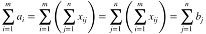
Equation (4.53) state that the total amount of the commodity transported from the origin i to the various destinations must be equal to the amount available at origin i (i = 1, 2, …, m), while Eq. (4.54) state that the total amount of the commodity received by destination j from all the sources must be equal to the amount required at the destination j (j = 1, 2, …, n). The nonnegativity conditions Eq. (4.55) are added since negative values for any x ij have no physical meaning. It is assumed that the total demand equals the total supply, that is,

Equation (4.56), called the consistency condition, must be satisfied if a solution is to exist. This can be seen easily since
The problem stated in Eqs. (4.52)-(4.56) was originally formulated and solved by Hitchcock in 1941 [6]. This was also considered independently by Koopmans in 1947 [7]. Because of these early investigations the problem is sometimes called the Hitchcock–Koopmans transportation problem. The special structure of the transportation matrix can be seen by writing the equations in standard form:


We notice the following properties from Eq. (4.58):
- All the nonzero coefficients of the constraints are equal to 1.
- The constraint coefficients appear in a triangular form.
- Any variable appears only once in the first m equations and once in the next n equations.
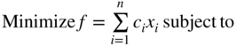
These are the special properties of the transportation problem that allow development of the transportation technique. To facilitate the identification of a starting solution, the system of equations (4.58) is represented in the form of an array, called the transportation array, as shown in Figure 4.2. In all the techniques developed for solving the transportation problem, the calculations are made directly on the transportation array.

Figure 4.2 Transportation array.
Computational Procedure. The solution of a LP problem, in general, requires a calculator or, if the problem is large, a high‐speed digital computer. On the other hand, the solution of a transportation problem can often be obtained with the use of a pencil and paper since additions and subtractions are the only calculations required. The basic steps involved in the solution of a transportation problem are
- Determine a starting basic feasible solution.
- Test the current basic feasible solution for optimality. If the current solution is optimal, stop the iterative process; otherwise, go to step 3.
- Select a variable to enter the basis from among the current nonbasic variables.
- Select a variable to leave from the basis from among the current basic variables (using the feasibility condition).
- Find a new basic feasible solution and return to step 2.
The details of these steps are given in Ref. [10].
4.7 Karmarkar's Interior Method
Karmarkar proposed a new method in 1984 for solving large‐scale linear programming problems very efficiently. The method is known as an interior method since it finds improved search directions strictly in the interior of the feasible space. This is in contrast with the simplex method, which searches along the boundary of the feasible space by moving from one feasible vertex to an adjacent one until the optimum point is found. For large LP problems, the number of vertices will be quite large and hence the simplex method would become very expensive in terms of computer time. Along with many other applications, Karmarkar's method has been applied to aircraft route scheduling problems. It was reported [19] that Karmarkar's method solved problems involving 150 000 design variables and 12 000 constraints in one hour while the simplex method required four hours for solving a smaller problem involving only 36 000 design variables and 10 000 constraints. In fact, it was found that Karmarkar's method is as much as 50 times faster than the simplex method for large problems.
Karmarkar's method is based on the following two observations:
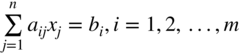
- If the current solution is near the center of the polytope, we can move along the steepest descent direction to reduce the value of f by a maximum amount. From Figure 4.3, we can see that the current solution can be improved substantially by moving along the steepest descent direction if it is near the center (point 2) but not near the boundary point (points 1 and 3).
- The solution space can always be transformed without changing the nature of the problem so that the current solution lies near the center of the polytope.

Figure 4.3 Improvement of objective function from different points of a polytope.
It is well known that in many numerical problems, by changing the units of data or rescaling (e.g. using feet instead of inches), we may be able to reduce the numerical instability. In a similar manner, Karmarkar observed that the variables can be transformed (in a more general manner than ordinary rescaling) so that straight lines remain straight lines while angles and distances change for the feasible space.
4.7.1 Statement of the Problem
Karmarkar's method requires the LP problem in the following form:
subject to

where X = {x 1 , x 2 ,…, x n }T , c = {c 1 ,c 2 ,…,c n }T, and [a] is an m × n matrix. In addition, an interior feasible starting solution to Eq. (4.59) must be known. Usually,

is chosen as the starting point. In addition, the optimum value of f must be zero for the problem. Thus

Although most LP problems may not be available in the form of Eq. (4.59) while satisfying the conditions of Eq. (4.60), it is possible to put any LP problem in a form that satisfies Eqs. (4.59) and (4.60) as indicated below.
4.7.2 Conversion of an LP Problem into the Required Form
Let the given LP problem be of the form
subject to

To convert this problem into the form of Eq. (4.59), we use the procedure suggested in Ref. [20] and define integers m and n such that X will be an (n − 3)‐component vector and [α] will be a matrix of order m − 1 × n − 3. We now define the vector ![]() = {z
1
, z
2
,···, z
n−3}T as
= {z
1
, z
2
,···, z
n−3}T as

where β is a constant chosen to have a sufficiently large value such that

for any feasible solution X (assuming that the solution is bounded). By using Eq. (4.62), the problem of Eq. (4.61) can be stated as follows:
subject to

We now define a new vector z as
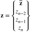
and solve the following related problem instead of the problem in Eq. (4.64):
subject to
where e is an (m − 1)‐component vector whose elements are all equal to 1, z
n−2 is a slack variable that absorbs the difference between 1 and the sum of other variables, z
n−1 is constrained to have a value of 1/n, and M is given a large value (corresponding to the artificial variable z
n
) to force z
n
to zero when the problem stated in Eq. (4.61) has a feasible solution. Eq. (4.65) are developed such that if z is a solution to these equations, X = β
![]() will be a solution to Eq. (4.61) if Eq. (4.61) have a feasible solution. Also, it can be verified that the interior point z = (1/n)
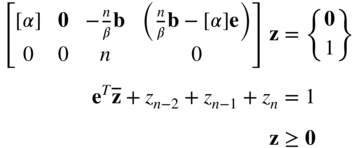
e is a feasible solution to Eq. (4.65). Equation (4.65) can be seen to be the desired form of Eq. (4.61) except for a 1 on the right‐hand side. This can be eliminated by subtracting the last constraint from the next‐to‐last constraint, to obtain the required form:
will be a solution to Eq. (4.61) if Eq. (4.61) have a feasible solution. Also, it can be verified that the interior point z = (1/n)
e is a feasible solution to Eq. (4.65). Equation (4.65) can be seen to be the desired form of Eq. (4.61) except for a 1 on the right‐hand side. This can be eliminated by subtracting the last constraint from the next‐to‐last constraint, to obtain the required form:
subject to
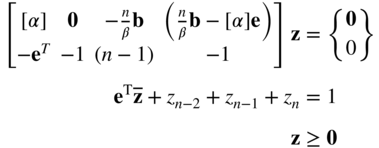
Note: When Eq. (4.66) are solved, if the value of the artificial variable z n > 0, the original problem in Eq. (4.61) is infeasible. On the other hand, if the value of the slack variable z n−2 = 0, the solution of the problem given by Eq. (4.61) is unbounded.
4.7.3 Algorithm
Starting from an interior feasible point X (1), Karmarkar's method finds a sequence of points X (2) , X (3) , ··· using the following iterative procedure:
- Initialize the iterative process. Begin with the center point of the simplex as the initial feasible point

Set the iteration number as k = 1.
- Test for optimality. Since f = 0 at the optimum point, we stop the procedure if the following convergence criterion is satisfied:
(4.67)

where ε is a small number. If Eq. (4.67) is not satisfied, go to step 3.
- Compute the next point, X
(k+1). For this, we first find a point Y
(k+1) in the transformed unit simplex as
(4.68)
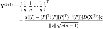
where ||c|| is the length of the vector c, [I] the identity matrix of order n, [D(X (k))] an n × n matrix with all off‐diagonal entries equal to 0, and diagonal entries equal to the components of the vector X (k) as
(4.69)
[P] is an (m + 1) × n matrix whose first m rows are given by [a] [D(X (k))] and the last row is composed of 1's:
(4.70)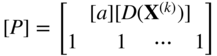
and the value of the parameter α is usually chosen as α =
 to ensure convergence. Once Y
(k+1) is found, the components of the new point X
(k+1) are determined as(4.71)
to ensure convergence. Once Y
(k+1) is found, the components of the new point X
(k+1) are determined as(4.71)
Set the new iteration number as k = k + 1 and go to step 2.
4.8 Quadratic Programming
A quadratic programming problem can be stated as
subject to
where
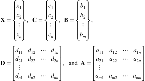
In Eq. (4.72) the term
X
T
DX
/2 represents the quadratic part of the objective function with D being a symmetric positive‐definite matrix. If D = 0, the problem reduces to a LP problem. The solution of the quadratic programming problem stated in Eqs. (4.72)-(4.74) can be obtained by using the Lagrange multiplier technique. By introducing the slack variables ![]() , i = 1, 2, …, m, in Eq. (4.73) and the surplus variables
, i = 1, 2, …, m, in Eq. (4.73) and the surplus variables ![]() , j = 1, 2, ..., n, in Eq. (4.74), the quadratic programming problem can be written as (see Eq. (4.72)) subject to the equality constraints
, j = 1, 2, ..., n, in Eq. (4.74), the quadratic programming problem can be written as (see Eq. (4.72)) subject to the equality constraints
where

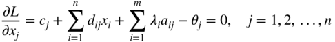
The Lagrange function can be written as

The necessary conditions for the stationariness of L give


By defining a set of new variables Y i as
Equation (4.81) can be written as
Multiplying Eq. (4.79) by s i and Eq. (4.80) by t j , we obtain
Combining Eqs. (4.84) and (4.85), and Eqs. (4.82) and (4.86), we obtain
Thus, the necessary conditions can be summarized as follows:
We can notice one important thing in Eqs. (4.89)-(4.96). With the exception of Eqs. (4.95) and (4.96), the necessary conditions are linear functions of the variables x j , Y i , λ i , and θ j . Thus, the solution of the original quadratic programming problem can be obtained by finding a nonnegative solution to the set of m + n linear equations given by Eqs. (4.89) and (4.90), which also satisfies the m + n equations stated in Eqs. (4.95) and (4.96).
Since D is a positive‐definite matrix, f (X) will be a strictly convex function,6 and the feasible space is convex (because of linear equations), any local minimum of the problem will be the global minimum. Further, it can be seen that there are 2 (n + m) variables and 2 (n + m) equations in the necessary conditions stated in Eqs. (4.89)-(4.96). Hence the solution of the Eqs. must be unique. Thus, the feasible solution satisfying all the Eqs. (4.89)-(4.96), if it exists, must give the optimum solution of the quadratic programming problem directly. The solution of the system of equations above can be obtained by using phase I of the simplex method. The only restriction here is that the satisfaction of the nonlinear relations, Eqs. (4.95) and (4.96), has to be maintained all the time. Since our objective is just to find a feasible solution to the set of Eqs. (4.89)-(4.96), there is no necessity of phase II computations. We shall follow the procedure developed by Wolfe [21] to apply phase I. This procedure involves the introduction of n nonnegative artificial variables z i into the Eq. (4.89) so that

Then we minimize

subject to the constraints

While solving this problem, we have to take care of the additional conditions
Thus, when deciding whether to introduce Y i into the basic solution, we first have to ensure that either λ i is not in the solution or λ i will be removed when Y i enters the basis. Similar care has to be taken regarding the variables θ j and x j . These additional checks are not very difficult to make during the solution procedure.
4.9 Solutions Using Matlab
The solution of different types of optimization problems using MATLAB is presented in Chapter 17. Specifically, the MATLAB solution of a linear programming problem using the interior point method is given in Example 17.3. Also, the MATLAB solution of a quadratic programming problem (given in Example 4.14) is presented as Example 17.4.
References and Bibliography
- 1 Gass, S. (1964). Linear Programming. New York: McGraw‐Hill.
- 2 Lemke, C.E. (1954). The dual method of solving the linear programming problem. Naval Research and Logistics Quarterly 1: 36–47.
- 3 Dantzig, G.B., Ford, L.R., and Fulkerson, D.R. (1956). A primal–dual algorithm for linear programs. In: Linear Inequalities and Related Systems, Annals of Mathematics Study No. 38 (eds. H.W. Kuhn and A.W. Tucker), 171–181. Princeton, NJ: Princeton University Press.
- 4 Dantzig, G.B. and Wolfe, P. (1960). Decomposition principle for linear programming. Operations Research 8: 101–111.
- 5 Lasdon, L.S. (1970). Optimization Theory for Large Systems. New York: Macmillan.
- 6 Hitchcock, F.L. (1941). The distribution of a product from several sources to numerous localities. Journal of Mathematical Physics 20: 224–230.
- 7 T. C. Koopmans, (1947). Optimum utilization of the transportation system, Proceedings of the International Statistical Conference, Washington, DC.
- 8 Zukhovitskiy, S. and Avdeyeva, L. (1966). Linear and Convex Programming, 147–155. Philadelphia: W. B. Saunders.
- 9 Garvin, W.W. (1960). Introduction to Linear Programming. New York: McGraw‐Hill.
- 10 Dantzig, G.B. (1963). Linear Programming and Extensions. Princeton, NJ: Princeton University Press.
- 11 Lemke, C.E. (1968). On complementary pivot theory. In: Mathematics of the Decision Sciences (eds. G.B. Dantzig and A.F. Veinott), Part 1, 95–136. Providence, RI: American Mathematical Society.
- 12 Murty, K. (1976). Linear and Combinatorial Programming. New York: Wiley.
- 13 Bitran, G.R. and Novaes, A.G. (1973). Linear programming with a fractional objective function. Operations Research 21: 22–29.
- 14 Choo, E.U. and Atkins, D.R. (1982). Bicriteria linear fractional programming. Journal of Optimization Theory and Applications 36: 203–220.
- 15 Singh, C. (1981). Optimality conditions in fractional programming. Journal of Optimization Theory and Applications 33: 287–294.
- 16 Lasserre, J.B. (1981). A property of certain multistage linear programs and some applications. Journal of Optimization Theory and Applications 34: 197–205.
- 17 Cohen, G. (1978). Optimization by decomposition and coordination: a unified approach. IEEE Transactions on Automatic Control 23: 222–232.
- 18 Karmarkar, N. (1984). A new polynomial‐time algorithm for linear programming. Combinatorica 4 (4): 373–395.
- 19 Winston, W.L. (1991). Operations Research Applications and Algorithms, 2e. Boston: PWS‐Kent.
- 20 Hooker, J.N. (1986). Karmarkar's linear programming algorithm. Interfaces 16 (4): 75–90.
- 21 Wolfe, P. (1959). The simplex method for quadratic programming. Econometrica 27: 382–398.
- 22 Boot, J.C.G. (1964). Quadratic Programming. Amsterdam: North‐Holland.
- 23 Van de Panne, C. (1974). Methods for Linear and Quadratic Programming. Amsterdam: North‐Holland.
- 24 Van de Panne, C. and Whinston, A. (1969). The symmetric formulation of the simplex method for quadratic programming. Econometrica 37: 507–527.
Review Questions
- 4.1 Is the decomposition method efficient for all LP problems?
- 4.2 What is the scope of postoptimality analysis?
- 4.3 Why is Karmarkar's method called an interior method?
- 4.4 What is the major difference between the simplex and Karmarkar methods?
- 4.5 State the form of LP problem required by Karmarkar's method.
- 4.6 What are the advantages of the revised simplex method?
- 4.7 Match the following terms and descriptions:
(a) Karmarkar's method Moves from one vertex to another (b) Simplex method Interior point algorithm (c) Quadratic programming Phase I computations not required (d) Dual simplex method Dantzig and Wolfe method (e) Decomposition method Wolfe's method - 4.8
Answer true or false:
- The quadratic programming problem is a convex programming problem.
- It is immaterial whether a given LP problem is designated the primal or dual.
- If the primal problem involves minimization of f subject to greater‐than constraints, its dual deals with the minimization of f subject to less‐than constraints.
- If the primal problem has an unbounded solution, its dual will also have an unbounded solution.
- The transportation problem can be solved by simplex method.
- 4.9 Match the following in the context of duality theory:
(a) x i is nonnegative
x i is unrestrictedith constraint is of less‐than or equal‐to type
Maximization type(b) ith constraint is of equality type ith variable is unrestricted (c) ith constraint is of greater‐than or equal‐to type ith variable is nonnegative (d) Minimization type ith constraint is of equality type
Problems
Solve LP problems 4.1–4.3 by the revised simplex method.
- 4.1
subject to


- 4.2
subject to


- 4.3
subject to


- 4.4 Discuss the relationships between the regular simplex method and the revised simplex method.
- 4.5 Solve the following LP problem graphically and by the revised simplex method:

subject to

- 4.6 Consider the following LP problem:

subject to

Solve this problem using the dual simplex method.
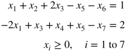
- 7 subject to

- Write the dual of this problem.
- Find the optimum solution of the dual.
- Verify the solution obtained in part (b) by solving the primal problem graphically.
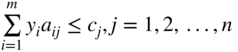
- 4.8 A water resource system consisting of two reservoirs is shown in Figure 4.4. The flows and storages are expressed in a consistent set of units. The following data are available:
Quantity Stream 1 (i = 1) Stream 2 (i = 2) Capacity of reservoir i 9 7 Available release from reservoir i 9 6 Capacity of channel below reservoir i 4 4 Actual release from reservoir i x 1 x 2 
Figure 4.4 Water resource system.
The capacity of the main channel below the confluence of the two streams is 5 units. If the benefit is equivalent to $2 × 10⁶ and $3 × 10⁶ per unit of water released from reservoirs 1 and 2, respectively, determine the releases x 1 and x 2 from the reserovirs to maximize the benefit. Solve this problem using duality theory.
- 4.9 Solve the following LP problem by the dual simplex method:

subject to
- 4.10 Solve Problem 3.1 by solving its dual.
- 4.11 Show that neither the primal nor the dual of the problem

subject to
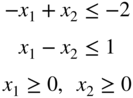
has a feasible solution. Verify your result graphically.
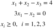
- 4.12 Solve the following LP problem by decomposition principle, and verify your result by solving it by the revised simplex method:

subject to

- 4.13 Apply the decomposition principle to the dual of the following problem and solve it:

subject to

- 4.14 Express the dual of the following LP problem:

subject to

- 4.15
Find the effect of changing b =
 to
to  in Example 4.5 using sensitivity analysis.
 - 4.16 Find the effect of changing the cost coefficients c 1 and c 4 from −45 and −50 to −40 and −60, respectively, in Example 4.5 using sensitivity analysis.
- 4.17 Find the effect of changing c 1 from −45 to −40 and c 2 from −100 to −90 in Example 4.5 using sensitivity analysis.
- 4.18 If a new product, E, which requires 10 minutes of work on lathe and 10 minutes of work on milling machine per unit, with a profit of $120 per unit is available in Example 4.5, determine whether it is worth manufacturing E.
- 4.19 A metallurgical company produces four products, A, B, C, and D, by using copper and zinc as basic materials. The material requirements and the profit per unit of each of the four products, and the maximum quantities of copper and zinc available are given below:
Product A B C D Maximum quantity available Copper (lb) 4 9 7 10 6000 Zinc (lb) 2 1 3 20 4000 Profit per unit ($) 15 25 20 60 Find the number of units of the various products to be produced for maximizing the profit.
- 4.20 Find the effect of changing the profit per unit of product D to $30.
- 4.21 Find the effect of changing the profit per unit of product A to $10, and of product B to $20.
- 4.22 Find the effect of changing the profit per unit of product B to $30 and of product C to $25.
- 4.23 Find the effect of changing the available quantities of copper and zinc to 4000 and 6000 lb, respectively.
- 4.24 What is the effect of introducing a new product, E, which requires 6 lb of copper and 3 lb of zinc per unit if it brings a profit of $30 per unit?
- 4.25 Assume that products A, B, C, and D require, in addition to the stated amounts of copper and zinc, 4, 3, 2 and 5 lb of nickel per unit, respectively. If the total quantity of nickel available is 2000 lb, in what way the original optimum solution is affected?
- 4.26 If product A requires 5 lb of copper and 3 lb of zinc (instead of 4 lb of copper and 2 lb of zinc) per unit, find the change in the optimum solution.
- 4.27 If product C requires 5 lb of copper and 4 lb of zinc (instead of 7 lb of copper and 3 lb of zinc) per unit, find the change in the optimum solution.
- 4.28 If the available quantities of copper and zinc are changed to 8000 and 5000 lb, respectively, find the change in the optimum solution.
- 4.29 Solve the following LP problem:

subject to
Investigate the change in the optimum solution of Problem 29 when the following changes are made (a) by using sensitivity analysis and (b) by solving the new problem graphically:
-
- 4.30 b 1 = 2
- 4.31 b 2 = 4
- 4.32 c 1 = 10
- 4.33 c 2 = −4
- 4.34 a 11 = −5
- 4.35 a 22 = −2
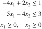
- 4.36 Perform one iteration of Karmarkar's method for the LP problem:

subject to

- 4.37 Perform one iteration of Karmarkar's method for the following LP problem:

subject to

- 4.38 Transform the following LP problem into the form required by Karmarkar's method:

subject to
- 4.39
A contractor has three sets of heavy construction equipment available at both New York and Los Angeles. He has construction jobs in Seattle, Houston, and Detroit that require two, three, and one set of equipment, respectively. The shipping costs per set between cities i and j (c
ij
) are shown in Figure 4.5. Formulate the problem of finding the shipping pattern that minimizes the cost.

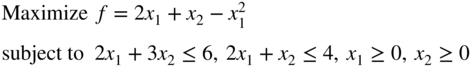
Figure 4.5 Shipping costs between cities. - 4.40

subject to

by quadratic programming.
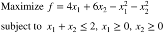
- 4.41 Find the solution of the quadratic programming problem stated in Example 1.5.
- 4.42
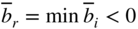
According to elastic–plastic theory, a frame structure fails (collapses) due to the formation of a plastic hinge mechanism. The various possible mechanisms in which a portal frame (Figure 4.6) can fail are shown in Figure 4.7. The reserve strengths of the frame in various failure mechanisms (Z
i
) can be expressed in terms of the plastic moment capacities of the hinges as indicated in Figure 4.7. Assuming that the cost of the frame is proportional to 200 times each of the moment capacities M
1
, M
2
, M
6, and M
7, and 100 times each of the moment capacities M
3
, M
4, and M
5, formulate the problem of minimizing the total cost to ensure nonzero reserve strength in each failure mechanism. Also, suggest a suitable technique for solving the problem. Assume that the moment capacities are restricted as 0 ≤ M
i
≤ 2 × 10⁵ lb‐in., i = 1, 2,…, 7. Data: x = 100 in., y = 150 in., P
1 = 1000 lb., and P
2 = 500 lb.
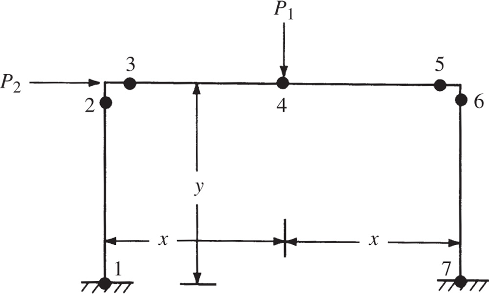
Figure 4.7 Plastic hinges in a frame. 
Figure 4.6 Possible failure mechanisms of a portal frame.
- 4.43 Solve the LP problem stated in Problem 9 using MATLAB (interior method).
- 4.44 Solve the LP problem stated in Problem 12 using MATLAB (interior method).
- 4.45 Solve the LP problem stated in Problem 13 using MATLAB (interior method).
- 4.46 Solve the LP problem stated in Problem 36 using MATLAB (interior method).
- 4.47 Solve the LP problem stated in Problem 37 using MATLAB (interior method).
- 4.48
Solve the following quadratic programming problem using MATLAB:
- 4.49
Solve the following quadratic programming problem using MATLAB:
- 4.50
Solve the following quadratic programming problem using MATLAB:

- 4.51
Solve the following quadratic programming problem using MATLAB:
