6
Nonlinear Programming II: Unconstrained Optimization Techniques
6.1 Introduction
This chapter deals with the various methods of solving the unconstrained minimization problem:

It is true that rarely a practical design problem would be unconstrained; still, a study of this class of problems is important for the following reasons:
- The constraints do not have significant influence in certain design problems.
- Some of the powerful and robust methods of solving constrained minimization problems require the use of unconstrained minimization techniques.
- The study of unconstrained minimization techniques provide the basic understanding necessary for the study of constrained minimization methods.
- The unconstrained minimization methods can be used to solve certain complex engineering analysis problems. For example, the displacement response (linear or nonlinear) of any structure under any specified load condition can be found by minimizing its potential energy. Similarly, the eigenvalues and eigenvectors of any discrete system can be found by minimizing the Rayleigh quotient.
As discussed in Chapter 2, a point X * will be a relative minimum of f(X) if the necessary conditions

are satisfied. The point X * is guaranteed to be a relative minimum if the Hessian matrix is positive definite, that is,

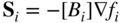
Equations (6.2) and (6.3) can be used to identify the optimum point during numerical computations. However, if the function is not differentiable, Eqs. (6.2) and (6.3) cannot be applied to identify the optimum point. For example, consider the function

where a > 0 and b > 0. The graph of this function is shown in Figure 6.1. It can be seen that this function is not differentiable at the minimum point, x * = 0, and hence Eqs. (6.2) and (6.3) are not applicable in identifying x *. In all such cases, the commonly understood notion of a minimum, namely, f(X *) < f(X) for all X, can be used only to identify a minimum point. The following example illustrates the formulation of a typical analysis problem as an unconstrained minimization problem.
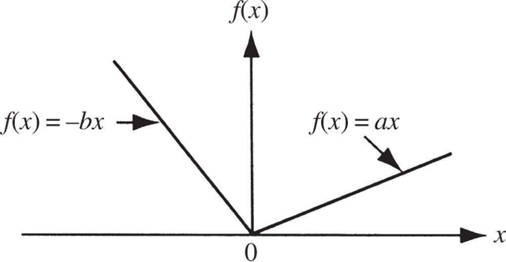
Figure 6.1 Function is not differentiable at minimum point.
6.1.1 Classification of Unconstrained Minimization Methods
Several methods are available for solving an unconstrained minimization problem. These methods can be classified into two broad categories as direct search methods and descent methods as indicated in Table 6.1. The direct search methods require only the objective function values but not the partial derivatives of the function in finding the minimum and hence are often called the nongradient methods. The direct search methods are also known as zeroth‐order methods since they use zeroth‐order derivatives of the function. These methods are most suitable for simple problems involving a relatively small number of variables. These methods are, in general, less efficient than the descent methods. The descent techniques require, in addition to the function values, the first and in some cases the second derivatives of the objective function. Since more information about the function being minimized is used (through the use of derivatives), descent methods are generally more efficient than direct search techniques. The descent methods are known as gradient methods. Among the gradient methods, those requiring only first derivatives of the function are called first‐order methods; those requiring both first and second derivatives of the function are termed second‐order methods.
Table 6.1 Unconstrained minimization methods.
| Direct search methodsa | Descent methodsb |
| Random search method | Steepest descent (Cauchy) method |
| Grid search method | Fletcher–Reeves method |
| Univariate method | Newton's method |
| Pattern search methods | Marquardt method |
| Powell's method | Quasi‐Newton methods |
| Davidon–Fletcher–Powell method | |
| Broyden–Fletcher–Goldfarb–Shanno method | |
| Simplex method |
a Do not require the derivatives of the function.
b Require the derivatives of the function.
6.1.2 General Approach
All the unconstrained minimization methods are iterative in nature and hence they start from an initial trial solution and proceed toward the minimum point in a sequential manner as shown in Figure 5.3. The iterative process is given by
where X
i
is the starting point, S
i
is the search direction, ![]() is the optimal step length, and X
i+1 is the final point in iteration i. It is important to note that all the unconstrained minimization methods (i) require an initial point X
1 to start the iterative procedure, and (ii) differ from one another only in the method of generating the new point X
i+1 (from X
i
) and in testing the point X
i+1 for optimality.
is the optimal step length, and X
i+1 is the final point in iteration i. It is important to note that all the unconstrained minimization methods (i) require an initial point X
1 to start the iterative procedure, and (ii) differ from one another only in the method of generating the new point X
i+1 (from X
i
) and in testing the point X
i+1 for optimality.
6.1.3 Rate of Convergence
Different iterative optimization methods have different rates of convergence. In general, an optimization method is said to have convergence of order p if 2

where X i and X i+1 denote the points obtained at the end of iterations i and i + 1, respectively, X * represents the optimum point, and ||X|| denotes the length or norm of the vector X:
If p = 1 and 0 ≤ k ≤ 1, the method is said to be linearly convergent (corresponds to slow convergence). If p = 2, the method is said to be quadratically convergent (corresponds to fast convergence). An optimization method is said to have superlinear convergence (corresponds to fast convergence) if

The definitions of rates of convergence given in Eqs. (6.5) and (6.6) are applicable to single‐variable as well as multivariable optimization problems. In the case of single‐variable problems, the vector, X i , for example, degenerates to a scalar, x i .
6.1.4 Scaling of Design Variables
The rate of convergence of most unconstrained minimization methods can be improved by scaling the design variables. For a quadratic objective function, the scaling of the design variables changes the condition number1 of the Hessian matrix. When the condition number of the Hessian matrix is 1, the steepest descent method, for example, finds the minimum of a quadratic objective function in one iteration.
If ![]() denotes a quadratic term, a transformation of the form
denotes a quadratic term, a transformation of the form
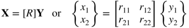
can be used to obtain a new quadratic term as
The matrix [R] can be selected to make [Ã] = [R]T[A][R] diagonal (i.e. to eliminate the mixed quadratic terms). For this, the columns of the matrix [R] are to be chosen as the eigenvectors of the matrix [A]. Next the diagonal elements of the matrix [Ã] can be reduced to 1 (so that the condition number of the resulting matrix will be 1) by using the transformation
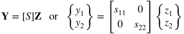
where the matrix [S] is given by

Thus the complete transformation that reduces the Hessian matrix of f to an identity matrix is given by
so that the quadratic term ![]() reduces to
reduces to ![]() .
.
If the objective function is not a quadratic, the Hessian matrix and hence the transformations vary with the design vector from iteration to iteration. For example, the second‐order Taylor's series approximation of a general nonlinear function at the design vector X i can be expressed as
where


The transformations indicated by Eqs. (6.7) and (6.9) can be applied to the matrix [A] given by Eq. (6.15). The procedure of scaling the design variables is illustrated with the following example.
Direct Search Methods
6.2 Random Search Methods
Random search methods are based on the use of random numbers in finding the minimum point. Since most of the computer libraries have random number generators, these methods can be used quite conveniently. Some of the best known random search methods are presented in this section.
6.2.1 Random Jumping Method
Although the problem is an unconstrained one, we establish the bounds l i and u i for each design variable x i , i = 1, 2, …, n, for generating the random values of x i :
In the random jumping method, we generate sets of n random numbers (r 1, r 2, …, r n ), that are uniformly distributed between 0 and 1. Each set of these numbers is used to find a point, X, inside the hypercube defined by Eq. (6.16) as

and the value of the function is evaluated at this point X. By generating a large number of random points X and evaluating the value of the objective function at each of these points, we can take the smallest value of f(X) as the desired minimum point.
6.2.2 Random Walk Method
The random walk method is based on generating a sequence of improved approximations to the minimum, each derived from the preceding approximation. Thus if X i is the approximation to the minimum obtained in the (i − 1)th stage (or step or iteration), the new or improved approximation in the ith stage is found from the relation
where λ is a prescribed scalar step length and u i is a unit random vector generated in the ith stage. The detailed procedure of this method is given by the following steps 3:
- Start with an initial point X 1, a sufficiently large initial step length λ, a minimum allowable step length ε, and a maximum permissible number of iterations N.
- Find the function value f 1 = f(X 1).
- Set the iteration number as i = 1.
- Generate a set of n random numbers r
1, r
2, …, r
n
each lying in the interval [−1, 1] and formulate the unit vector u as
(6.19)
The directions generated using Eq. (6.19) are expected to have a bias toward the diagonals of the unit hypercube 3. To avoid such a bias, the length of the vector, R, is computed as

and the random numbers generated (r 1, r 2, …, r n ) are accepted only if R ≤ 1 but are discarded if R > 1. If the random numbers are accepted, the unbiased random vector u i is given by Eq. (6.19).
- Compute the new vector and the corresponding function value as X = X 1 + λ u and f = f(X).
- Compare the values of f and f 1. If f < f 1, set the new values as X 1 = X and f 1 = f and go to step 3. If f ≥ f 1, go to step 7.
- If i ≤ N, set the new iteration number as i = i + 1 and go to step 4. On the other hand, if i > N, go to step 8.
- Compute the new, reduced, step length as λ = λ/2. If the new step length is smaller than or equal to ε, go to step 9. Otherwise (i.e. if the new step length is greater than ε), go to step 4.
- Stop the procedure by taking X opt ≈ X 1 and f opt ≈ f 1.
This method is illustrated with the following example.
6.2.3 Random Walk Method with Direction Exploitation
In the random walk method described in Section 6.2.2, we proceed to generate a new unit random vector u i+1 as soon as we find that u i is successful in reducing the function value for a fixed step length λ. However, we can expect to achieve a further decrease in the function value by taking a longer step length along the direction u i . Thus the random walk method can be improved if the maximum possible step is taken along each successful direction. This can be achieved by using any of the one‐dimensional minimization methods discussed in Chapter 5. According to this procedure, the new vector X i+1 is found as
where ![]() is the optimal step length found along the direction u
i
so that
is the optimal step length found along the direction u
i
so that
The search method incorporating this feature is called the random walk method with direction exploitation.
6.2.4 Advantages of Random Search Methods
- These methods can work even if the objective function is discontinuous and nondifferentiable at some of the points.
- The random methods can be used to find the global minimum when the objective function possesses several relative minima.
- These methods are applicable when other methods fail due to local difficulties such as sharply varying functions and shallow regions.
- Although the random methods are not very efficient by themselves, they can be used in the early stages of optimization to detect the region where the global minimum is likely to be found. Once this region is found, some of the more efficient techniques can be used to find the precise location of the global minimum point.
6.3 Grid Search Method
This method involves setting up a suitable grid in the design space, evaluating the objective function at all the gird points, and finding the grid point corresponding to the lowest function value. For example, if the lower and upper bounds on the ith design variable are known to be l
i
and u
i
, respectively, we can divide the range (l
i
, u
i
) into p
i
− 1 equal parts so that ![]() denote the grid points along the x
i
axis (i = 1, 2, …, n). This leads to a total of p
1
p
2 ⋯ p
n
grid points in the design space. A grid with p
i
= 4 is shown in a two‐dimensional design space in Figure 6.4. The grid points can also be chosen based on methods of experimental design 4,5. It can be seen that the grid method requires prohibitively large number of function evaluations in most practical problems. For example, for a problem with 10 design variables (n = 10), the number of grid points will be 310 = 59 049 with p
i
= 3 and 410 = 1 048 576 with p
i
= 4. However, for problems with a small number of design variables, the grid method can be used conveniently to find an approximate minimum. Also, the grid method can be used to find a good starting point for one of the more efficient methods.
denote the grid points along the x
i
axis (i = 1, 2, …, n). This leads to a total of p
1
p
2 ⋯ p
n
grid points in the design space. A grid with p
i
= 4 is shown in a two‐dimensional design space in Figure 6.4. The grid points can also be chosen based on methods of experimental design 4,5. It can be seen that the grid method requires prohibitively large number of function evaluations in most practical problems. For example, for a problem with 10 design variables (n = 10), the number of grid points will be 310 = 59 049 with p
i
= 3 and 410 = 1 048 576 with p
i
= 4. However, for problems with a small number of design variables, the grid method can be used conveniently to find an approximate minimum. Also, the grid method can be used to find a good starting point for one of the more efficient methods.

Figure 6.4 Grid with p i = 4.
6.4 Univariate Method
In this method we change only one variable at a time and seek to produce a sequence of improved approximations to the minimum point. By starting at a base point X i in the ith iteration, we fix the values of n − 1 variables and vary the remaining variable. Since only one variable is changed, the problem becomes a one‐dimensional minimization problem and any of the methods discussed in Chapter 5 can be used to produce a new base point X i+1. The search is now continued in a new direction. This new direction is obtained by changing any one of the n − 1 variables that were fixed in the previous iteration. In fact, the search procedure is continued by taking each coordinate direction in turn. After all the n directions are searched sequentially, the first cycle is complete and hence we repeat the entire process of sequential minimization. The procedure is continued until no further improvement is possible in the objective function in any of the n directions of a cycle. The univariate method can be summarized as follows:
- Choose an arbitrary staring point X 1 and set i = 1.
- Find the search direction S
i
as
(6.22)

- Determine whether λ i should be positive or negative. For the current direction S i , this means find whether the function value decreases in the positive or negative direction. For this we take a small probe length (ε) and evaluate f i = f(X i ), f + = f(X i + ε S i ), and f − = f(X i − ε S i ). If f + < f i , S i will be the correct direction for decreasing the value of f and if f − < f i , −S i will be the correct one. If both f + and f − are greater than f i , we take X i as the minimum along the direction S i .
- Find the optimal step length
 such that
(6.23)
such that
(6.23)
where + or − sign has to be used depending upon whether S i or −S i is the direction for decreasing the function value.
- Set
 depending on the direction for decreasing the function value, and f
i+1 = f(X
i+1).
depending on the direction for decreasing the function value, and f
i+1 = f(X
i+1). - Set the new value of i = i + 1 and go to step 2. Continue this procedure until no significant change is achieved in the value of the objective function.
The univariate method is very simple and can be implemented easily. However, it will not converge rapidly to the optimum solution, as it has a tendency to oscillate with steadily decreasing progress toward the optimum. Hence it will be better to stop the computations at some point near to the optimum point rather than trying to find the precise optimum point. In theory, the univariate method can be applied to find the minimum of any function that possesses continuous derivatives. However, if the function has a steep valley, the method may not even converge. For example, consider the contours of a function of two variables with a valley as shown in Figure 6.5. If the univariate search starts at point P, the function value cannot be decreased either in the direction ±S 1 or in the direction ±S 2. Thus the search comes to a halt and one may be misled to take the point P, which is certainly not the optimum point, as the optimum point. This situation arises whenever the value of the probe length ε needed for detecting the proper direction (±S 1 or ±S 2) happens to be less than the number of significant figures used in the computations.

Figure 6.5 Failure of the univariate method on a steep valley.
6.5 Pattern Directions
In the univariate method, we search for the minimum along directions parallel to the coordinate axes. We noticed that this method may not converge in some cases, and that even if it converges, its convergence will be very slow as we approach the optimum point. These problems can be avoided by changing the directions of search in a favorable manner instead of retaining them always parallel to the coordinate axes. To understand this idea, consider the contours of the function shown in Figure 6.6. Let the points 1, 2, 3, … indicate the successive points found by the univariate method. It can be noticed that the lines joining the alternate points of the search (e.g. 1, 3; 2, 4; 3, 5; 4, 6; …) lie in the general direction of the minimum and are known as pattern directions. It can be proved that if the objective function is a quadratic in two variables, all such lines pass through the minimum. Unfortunately, this property will not be valid for multivariable functions even when they are quadratics. However, this idea can still be used to achieve rapid convergence while finding the minimum of an n‐variable function. Methods that use pattern directions as search directions are known as pattern search methods.

Figure 6.6 Lines defined by the alternate points lie in the general direction of the minimum.
One of the best‐known pattern search methods, the Powell's method, is discussed in Section 6.6. In general, a pattern search method takes n univariate steps, where n denotes the number of design variables and then searches for the minimum along the pattern direction S i , defined by
where X i is the point obtained at the end of n univariate steps and X i−n is the starting point before taking the n univariate steps. In general, the directions used prior to taking a move along a pattern direction need not be univariate directions.
6.6 Powell's Method
Powell's method is an extension of the basic pattern search method. It is the most widely used direct search method and can be proved to be a method of conjugate directions 7. A conjugate directions method will minimize a quadratic function in a finite number of steps. Since a general nonlinear function can be approximated reasonably well by a quadratic function near its minimum, a conjugate directions method is expected to speed up the convergence of even general nonlinear objective functions. The definition, a method of generation of conjugate directions, and the property of quadratic convergence are presented in this section.
6.6.1 Conjugate Directions
-
Definition: Conjugate Directions. Let A = [A] be an n × n symmetric matrix. A set of n vectors (or directions) {S
i
} is said to be conjugate (more accurately A‐conjugate) if
(6.25)

It can be seen that orthogonal directions are a special case of conjugate directions (obtained with [A] = [I] in Eq. (6.25)).
- Definition: Quadratically Convergent Method. If a minimization method, using exact arithmetic, can find the minimum point in n steps while minimizing a quadratic function in n variables, the method is called a quadratically convergent method.
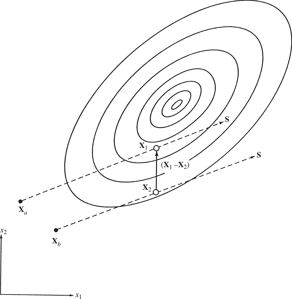
Figure 6.7 Conjugate directions.
6.6.2 Algorithm
The basic idea of Powell's method is illustrated graphically for a two‐variable function in Figure 6.8. In this figure the function is first minimized once along each of the coordinate directions starting with the second coordinate direction and then in the corresponding pattern direction. This leads to point 5. For the next cycle of minimization, we discard one of the coordinate directions (the x 1 direction in the present case) in favor of the pattern direction. Thus we minimize along u 2 and S 1 and obtain point 7. Then we generate a new pattern direction S 2 as shown in the figure. For the next cycle of minimization, we discard one of the previously used coordinate directions (the x 2 direction in this case) in favor of the newly generated pattern direction. Then, by starting from point 8, we minimize along directions S 1 and S 2, thereby obtaining points 9 and 10, respectively. For the next cycle of minimization, since there is no coordinate direction to discard, we restart the whole procedure by minimizing along the x 2 direction. This procedure is continued until the desired minimum point is found.

Figure 6.8 Progress of Powell's method.
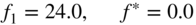
The flow diagram for the version of Powell's method described above is given in Figure 6.9. Note that the search will be made sequentially in the directions S
n
; S
1, S
2, S
3, …, S
n−1, S
n
; ![]() ; S
2, S
3, …, S
n−1, S
n
,
; S
2, S
3, …, S
n−1, S
n
, ![]() ;
; ![]() ; S
3, S
4, …, S
n−1, S
n
,
; S
3, S
4, …, S
n−1, S
n
, ![]() ,
, ![]() ;
; ![]() , … until the minimum point is found. Here S
i
indicates the coordinate direction u
i
and
, … until the minimum point is found. Here S
i
indicates the coordinate direction u
i
and ![]() the jth pattern direction. In Figure 6.9, the previous base point is stored as the vector Z in block A, and the pattern direction is constructed by subtracting the previous base point from the current one in block B. The pattern direction is then used as a minimization direction in blocks C and D. For the next cycle, the first direction used in the previous cycle is discarded in favor of the current pattern direction. This is achieved by updating the numbers of the search directions as shown in block E. Thus, both points Z and X used in block B for the construction of pattern direction are points that are minima along S
n
in the first cycle, the first pattern direction
the jth pattern direction. In Figure 6.9, the previous base point is stored as the vector Z in block A, and the pattern direction is constructed by subtracting the previous base point from the current one in block B. The pattern direction is then used as a minimization direction in blocks C and D. For the next cycle, the first direction used in the previous cycle is discarded in favor of the current pattern direction. This is achieved by updating the numbers of the search directions as shown in block E. Thus, both points Z and X used in block B for the construction of pattern direction are points that are minima along S
n
in the first cycle, the first pattern direction ![]() in the second cycle, the second pattern direction
in the second cycle, the second pattern direction ![]() in the third cycle, and so on.
in the third cycle, and so on.

Figure 6.9 Flowchart for Powell's Method.
Quadratic Convergence
It can be seen from Figure 6.9 that the pattern directions ![]() ,
, ![]() ,
, ![]() , … are nothing but the lines joining the minima found along the directions S
n
,
, … are nothing but the lines joining the minima found along the directions S
n
, ![]() ,
, ![]() , …, respectively. Hence by Theorem 6.1, the pairs of directions (S
n
,
, …, respectively. Hence by Theorem 6.1, the pairs of directions (S
n
, ![]() ), (
), (![]() ,
, ![]() ), and so on, are A‐conjugate. Thus, all the directions S
n
,
), and so on, are A‐conjugate. Thus, all the directions S
n
, ![]() ,
, ![]() , … are A‐conjugate. Since, by Theorem 6.2, any search method involving minimization along a set of conjugate directions is quadratically convergent, Powell's method is quadratically convergent. From the method used for constructing the conjugate directions
, … are A‐conjugate. Since, by Theorem 6.2, any search method involving minimization along a set of conjugate directions is quadratically convergent, Powell's method is quadratically convergent. From the method used for constructing the conjugate directions ![]() ,
, ![]() , …, we find that n minimization cycles are required to complete the construction of n conjugate directions. In the ith cycle, the minimization is done along the already constructed i conjugate directions and the n − i nonconjugate (coordinate) directions. Thus after n cycles, all the n search directions are mutually conjugate and a quadratic will theoretically be minimized in n
2 one‐dimensional minimizations. This proves the quadratic convergence of Powell's method.
, …, we find that n minimization cycles are required to complete the construction of n conjugate directions. In the ith cycle, the minimization is done along the already constructed i conjugate directions and the n − i nonconjugate (coordinate) directions. Thus after n cycles, all the n search directions are mutually conjugate and a quadratic will theoretically be minimized in n
2 one‐dimensional minimizations. This proves the quadratic convergence of Powell's method.
It is to be noted that as with most of the numerical techniques, the convergence in many practical problems may not be as good as the theory seems to indicate. Powell's method may require a lot more iterations to minimize a function than the theoretically estimated number. There are several reasons for this:
- Since the number of cycles n is valid only for quadratic functions, it will take generally greater than n cycles for nonquadratic functions.
- The proof of quadratic convergence has been established with the assumption that the exact minimum is found in each of the one‐dimensional minimizations. However, the actual minimizing step lengths
 will be only approximate, and hence the subsequent directions will not be conjugate. Thus the method requires more number of iterations for achieving the overall convergence.
 - Powell's method, described above, can break down before the minimum point is found. This is because the search directions S i might become dependent or almost dependent during numerical computation.
Convergence Criterion
The convergence criterion one would generally adopt in a method such as Powell's method is to stop the procedure whenever a minimization cycle produces a change in all variables less than one‐tenth of the required accuracy. However, a more elaborate convergence criterion, which is more likely to prevent premature termination of the process, was given by Powell 7.
6.7 Simplex Method
Definition: Simplex. The geometric figure formed by a set of n + 1 points in an n‐dimensional space is called a simplex. When the points are equidistant, the simplex is said to be regular. Thus, in two dimensions the simplex is a triangle, and in three dimensions, it is a tetrahedron.
The basic idea in the simplex method3 is to compare the values of the objective function at the n + 1 vertices of a general simplex and move the simplex gradually toward the optimum point during the iterative process. The following equations can be used to generate the vertices of a regular simplex (equilateral triangle in two‐dimensional space) of size a in the n‐dimensional space 10:

where

where X 0 is the initial base point and u j is the unit vector along the jth coordinate axis. This method was originally given by Spendley et al. 10 and was developed later by Nelder and Mead 11. The movement of the simplex is achieved by using three operations, known as reflection, contraction, and expansion.
6.7.1 Reflection
If X h is the vertex corresponding to the highest value of the objective function among the vertices of a simplex, we can expect the point X r obtained by reflecting the point X h in the opposite face to have the smallest value. If this is the case, we can construct a new simplex by rejecting the point X h from the simplex and including the new point X r . This process is illustrated in Figure 6.10. In Figure 6.10a, the points X 1, X 2, and X 3 form the original simplex, and the points X 1, X 2, and X r form the new one. Similarly, in Figure 6.10b, the original simplex is given by points X 1, X 2, X 3, and X 4, and the new one by X 1, X 2, X 3, and X r . Again, we can construct a new simplex from the present one by rejecting the vertex corresponding to the highest function value. Since the direction of movement of the simplex is always away from the worst result, we will be moving in a favorable direction. If the objective function does not have steep valleys, repetitive application of the reflection process leads to a zigzag path in the general direction of the minimum as shown in Figure 6.11. Mathematically, the reflected point X r is given by
where X h is the vertex corresponding to the maximum function value:

Figure 6.10 Reflection.

Figure 6.11 Progress of the reflection process.
X 0 is the centroid of all the points X i except i = h:

and α > 0 is the reflection coefficient defined as

Thus X r will lie on the line joining X h and X 0, on the far side of X 0 from X h with |X r − X 0| = α|X h − X 0|. If f(X r ) lies between f(X h ) and f(X l ), where X l is the vertex corresponding to the minimum function value,
X h is replaced by X r and a new simplex is started.
If we use only the reflection process for finding the minimum, we may encounter certain difficulties in some cases. For example, if one of the simplexes (triangles in two dimensions) straddles a valley as shown in Figure 6.12 and if the reflected point X r happens to have an objective function value equal to that of the point X h , we will enter into a closed cycle of operations. Thus if X 2 is the worst point in the simplex defined by the vertices X 1, X 2, and X 3, the reflection process gives the new simplex with vertices X 1, X 3, and X r . Again, since X r has the highest function value out of the vertices X 1, X 3, and X r , we obtain the old simplex itself by using the reflection process. Thus the optimization process is stranded over the valley and there is no way of moving toward the optimum point. This trouble can be overcome by making a rule that no return can be made to points that have just been left.

Figure 6.12 Reflection process not leading to a new simplex.
Whenever such situation is encountered, we reject the vertex corresponding to the second worst value instead of the vertex corresponding to the worst function value. This method, in general, leads the process to continue toward the region of the desired minimum. However, the final simplex may again straddle the minimum, or it may lie within a distance of the order of its own size from the minimum. In such cases it may not be possible to obtain a new simplex with vertices closer to the minimum compared to those of the previous simplex, and the pattern may lead to a cyclic process, as shown in Figure 6.13. In this example the successive simplexes formed from the simplex 123 are 234, 245, 456, 467, 478, 348, 234, 245, …,4 which can be seen to be forming a cyclic process. Whenever this type of cycling is observed, one can take the vertex that is occurring in every simplex (point 4 in Figure 6.13) as the best approximation to the optimum point. If more accuracy is desired, the simplex has to be contracted or reduced in size, as indicated later.

Figure 6.13 Reflection process leading to a cyclic process.
6.7.2 Expansion
If a reflection process gives a point X r for which f(X r ) < f(X l ) (i.e. if the reflection produces a new minimum), one can generally expect to decrease the function value further by moving along the direction pointing from X 0 to X r . Hence we expand X r to X e using the relation
where γ is called the expansion coefficient, defined as

If f(X e ) < f(X l ), we replace the point X h by X e and restart the process of reflection. On the other hand, if f(X e ) > f(X l ), it means that the expansion process is not successful and hence we replace point X h by X r and start the reflection process again.
6.7.3 Contraction
If the reflection process gives a point X r for which f(X r ) > f(X i ) for all i except i = h, and f(X r ) < f(X h ), we replace point X h by X r . Thus the new X h will be X r . In this case we contract the simplex as follows:
where β is called the contraction coefficient (0 ≤ β ≤ 1) and is defined as

If f(X r ) > f(X h ), we still use Eq. (6.54) without changing the previous point X h . If the contraction process produces a point X c for which f(X c ) < min[f(X h ), f(X r )], we replace the point X h in X 1, X 2, …, X n+1 by X c and proceed with the reflection process again. On the other hand, if f(X c ) ≥ min[f(X h ), f(X r )], the contraction process will be a failure, and in this case we replace all X i by (X i + X l )/2 and restart the reflection process.
The method is assumed to have converged whenever the standard deviation of the function at the n + 1 vertices of the current simplex is smaller than some prescribed small quantity ε, that is,

Indirect Search (Descent) Methods
6.8 Gradient of a Function
The gradient of a function is an n‐component vector given by

The gradient has a very important property. If we move along the gradient direction from any point in n‐dimensional space, the function value increases at the fastest rate. Hence the gradient direction is called the direction of steepest ascent. Unfortunately, the direction of steepest ascent is a local property and not a global one. This is illustrated in Figure 6.14, where the gradient vectors ∇f evaluated at points 1, 2, 3, and 4 lies along the directions 11′, 22′, 33′, and 44′, respectively. Thus the function value increases at the fastest rate in the direction 11′ at point 1, but not at point 2. Similarly, the function value increases at the fastest rate in direction 22′(33′) at point 2 (3), but not at point 3 (4). In other words, the direction of steepest ascent generally varies from point to point, and if we make infinitely small moves along the direction of steepest ascent, the path will be a curved line like the curve 1–2–3–4 in Figure 6.14.
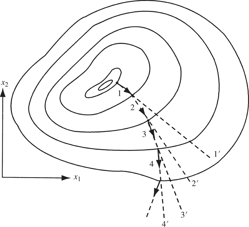
Figure 6.14 Steepest ascent directions.
Since the gradient vector represents the direction of steepest ascent, the negative of the gradient vector denotes the direction of steepest descent. Thus any method that makes use of the gradient vector can be expected to give the minimum point faster than one that does not make use of the gradient vector. All the descent methods make use of the gradient vector, either directly or indirectly, in finding the search directions. Before considering the descent methods of minimization, we prove that the gradient vector represents the direction of steepest ascent.
6.8.1 Evaluation of the Gradient
The evaluation of the gradient requires the computation of the partial derivatives ∂f/∂x i , i = 1, 2, …, n. There are three situations where the evaluation of the gradient poses certain problems:
- The function is differentiable at all the points, but the calculation of the components of the gradient, ∂f/∂x i , is either impractical or impossible.
- The expressions for the partial derivatives ∂f/∂x i can be derived, but they require large computational time for evaluation.
- The gradient ∇f is not defined at all the points.
In the first case, we can use the forward finite‐difference formula

to approximate the partial derivative ∂f/∂x i at X m . If the function value at the base point X m is known, this formula requires one additional function evaluation to find (∂f/∂x i )| Xm . Thus it requires n additional function evaluations to evaluate the approximate gradient ∇f| X m . For better results we can use the central finite difference formula to find the approximate partial derivative ∂f/∂x i | X m :

This formula requires two additional function evaluations for each of the partial derivatives. In Eqs. (6.63) and (6.64), Δx i is a small scalar quantity and u i is a vector of order n whose ith component has a value of 1, and all other components have a value of zero. In practical computations, the value of Δx i has to be chosen with some care. If Δx i is too small, the difference between the values of the function evaluated at (X m + Δx i u i ) and (X m − Δx i u i ) may be very small and numerical round‐off error may predominate. On the other hand, if Δx i is too large, the truncation error may predominate in the calculation of the gradient.
In the second case also, the use of finite‐difference formulas is preferred whenever the exact gradient evaluation requires more computational time than the one involved in using Eq. (6.63) or (6.64).
In the third case, we cannot use the finite‐difference formulas since the gradient is not defined at all the points. For example, consider the function shown in Figure 6.15. If Eq. (6.64) is used to evaluate the derivative df/ds at X m , we obtain a value of α 1 for a step size Δx 1 and a value of α 2 for a step size Δx 2. Since, in reality, the derivative does not exist at the point X m , use of finite‐difference formulas might lead to a complete breakdown of the minimization process. In such cases the minimization can be done only by one of the direct search techniques discussed earlier.

Figure 6.15 Gradient not defined at x m .
6.8.2 Rate of Change of a Function Along a Direction
In most optimization techniques, we are interested in finding the rate of change of a function with respect to a parameter λ along a specified direction, S i , away from a point X i . Any point in the specified direction away from the given point X i can be expressed as X = X i + λ S i . Our interest is to find the rate of change of the function along the direction S i (characterized by the parameter λ), that is,

where x j is the jth component of X. But
where x ij and s ij are the jth components of X i and S i , respectively. Hence
If λ * minimizes f in the direction S i , we have

at the point X i + λ * S i .
6.9 Steepest Descent (CAuchy) Method
The use of the negative of the gradient vector as a direction for minimization was first made by Cauchy in 1847 12. In this method we start from an initial trial point X 1 and iteratively move along the steepest descent directions until the optimum point is found. The steepest descent method can be summarized by the following steps:
- Start with an arbitrary initial point X 1. Set the iteration number as i = 1.
- Find the search direction S
i
as
(6.69)

- Determine the optimal step length
 in the direction S
i
and set
(6.70)
in the direction S
i
and set
(6.70)
- Test the new point, X i+1, for optimality. If X i+1 is optimum, stop the process. Otherwise, go to step 5.
- Set the new iteration number i = i + 1 and go to step 2.
The method of steepest descent may appear to be the best unconstrained minimization technique since each one‐dimensional search starts in the “best” direction. However, owing to the fact that the steepest descent direction is a local property, the method is not really effective in most problems.
6.10 Conjugate Gradient (FLetcher–REeves) Method
The convergence characteristics of the steepest descent method can be improved greatly by modifying it into a conjugate gradient method (which can be considered as a conjugate directions method involving the use of the gradient of the function). We saw (in Section 6.6) that any minimization method that makes use of the conjugate directions is quadratically convergent. This property of quadratic convergence is very useful because it ensures that the method will minimize a quadratic function in n steps or less. Since any general function can be approximated reasonably well by a quadratic near the optimum point, any quadratically convergent method is expected to find the optimum point in a finite number of iterations.
We have seen that Powell's conjugate direction method requires n single‐variable minimizations per iteration and sets up a new conjugate direction at the end of each iteration. Thus it requires, in general, n 2 single‐variable minimizations to find the minimum of a quadratic function. On the other hand, if we can evaluate the gradients of the objective function, we can set up a new conjugate direction after every one‐dimensional minimization, and hence we can achieve faster convergence. The construction of conjugate directions and development of the Fletcher–Reeves method are discussed in this section.
6.10.1 Development of the Fletcher–Reeves Method
The Fletcher–Reeves method is developed by modifying the steepest descent method to make it quadratically convergent. Starting from an arbitrary point X 1, the quadratic function
can be minimized by searching along the search direction S 1 = −∇f 1 (steepest descent direction) using the step length (see Problem 40):

The second search direction S 2 is found as a linear combination of S 1 and − ∇f 2:
where the constant β 2 can be determined by making S 1 and S 2 conjugate with respect to [A]. This leads to (see Problem 41):

This process can be continued to obtain the general formula for the ith search direction as
where
Thus the Fletcher–Reeves algorithm can be stated as follows.
6.10.2 Fletcher–Reeves Method
The iterative procedure of Fletcher–Reeves method can be stated as follows:
- Start with an arbitrary initial point X 1.
- Set the first search direction S 1 = −∇f(X 1) = −∇f 1.
- Find the point X
2 according to the relation
(6.80)

where
 is the optimal step length in the direction S
1. Set i = 2 and go to the next step.
is the optimal step length in the direction S
1. Set i = 2 and go to the next step. - Find ∇f
i
= ∇f(X
i
), and set
(6.81)

- Compute the optimum step length
 in the direction S
i
, and find the new point
(6.82)
in the direction S
i
, and find the new point
(6.82)
- Test for the optimality of the point X i+1. If X i+1 is optimum, stop the process. Otherwise, set the value of i = i + 1 and go to step 4.
Remarks
- The Fletcher–Reeves method was originally proposed by Hestenes and Stiefel 14 as a method for solving systems of linear equations derived from the stationary conditions of a quadratic. Since the directions S
i
used in this method are A‐conjugate, the process should converge in n cycles or less for a quadratic function. However, for ill‐conditioned quadratics (whose contours are highly eccentric and distorted), the method may require much more than n cycles for convergence. The reason for this has been found to be the cumulative effect of rounding errors. Since S
i
is given by Eq. (6.81), any error resulting from the inaccuracies involved in the determination of
 , and from the round‐off error involved in accumulating the successive |∇f
i
|2
S
i−1/|∇f
i−1|2 terms, is carried forward through the vector S
i
. Thus the search directions S
i
will be progressively contaminated by these errors. Hence it is necessary, in practice, to restart the method periodically after every, say, m steps by taking the new search direction as the steepest descent direction. That is, after every m steps, S
m+1 is set equal to −∇f
m+1 instead of the usual form. Fletcher and Reeves have recommended a value of m = n + 1, where n is the number of design variables.
, and from the round‐off error involved in accumulating the successive |∇f
i
|2
S
i−1/|∇f
i−1|2 terms, is carried forward through the vector S
i
. Thus the search directions S
i
will be progressively contaminated by these errors. Hence it is necessary, in practice, to restart the method periodically after every, say, m steps by taking the new search direction as the steepest descent direction. That is, after every m steps, S
m+1 is set equal to −∇f
m+1 instead of the usual form. Fletcher and Reeves have recommended a value of m = n + 1, where n is the number of design variables. - Despite the limitations indicated above, the Fletcher–Reeves method is vastly superior to the steepest descent method and the pattern search methods, but it turns out to be rather less efficient than the Newton and the quasi‐Newton (variable metric) methods discussed in the latter sections.
6.11 Newton's Method
Newton's method presented in Section 5.12.1 can be extended for the minimization of multivariable functions. For this, consider the quadratic approximation of the function f(X) at X = X i using the Taylor's series expansion
where [J i ] = [J]| X i is the matrix of second partial derivatives (Hessian matrix) of f evaluated at the point X i . By setting the partial derivatives of Eq. (6.83) equal to zero for the minimum of f(X), we obtain
Equations (6.84) and (6.83) give
If [J i ] is nonsingular, Eq. (6.85) can be solved to obtain an improved approximation (X = X i+1) as
Since higher‐order terms have been neglected in Eq. (6.83), Eq. (6.86) is to be used iteratively to find the optimum solution X*.
The sequence of points X 1, X 2, …, X i+1 can be shown to converge to the actual solution X* from any initial point X 1 sufficiently close to the solution X*, provided that [J 1] is nonsingular. It can be seen that Newton's method uses the second partial derivatives of the objective function (in the form of the matrix [J i ]) and hence is a second‐order method.
6.12 MArquardt Method
The steepest descent method reduces the function value when the design vector X i is away from the optimum point X*. The Newton method, on the other hand, converges fast when the design vector X i is close to the optimum point X*. The Marquardt method 15 attempts to take advantage of both the steepest descent and Newton methods. This method modifies the diagonal elements of the Hessian matrix, [J i ], as
where [I] is an identity matrix and α
i
is a positive constant that ensures the positive definiteness of [![]() ] when [J
i
] is not positive definite. It can be noted that when α
i
is sufficiently large (on the order of 104), the term α
i
[I] dominates [J
i
] and the inverse of the matrix [J
i
] becomes
] when [J
i
] is not positive definite. It can be noted that when α
i
is sufficiently large (on the order of 104), the term α
i
[I] dominates [J
i
] and the inverse of the matrix [J
i
] becomes
Thus if the search direction S i is computed as
S i becomes a steepest descent direction for large values of α i . In the Marquardt method, the value of α i is taken to be large at the beginning and then reduced to zero gradually as the iterative process progresses. Thus as the value of α i decreases from a large value to zero, the characteristics of the search method change from those of a steepest descent method to those of the Newton method. The iterative process of a modified version of Marquardt method can be described as follows.
- Start with an arbitrary initial point X 1 and constants α 1 (on the order of 104), c 1(0 < c 1 < 1), c 2(c 2 > 1), and ε (on the order of 10−2). Set the iteration number as i = 1.
- Compute the gradient of the function, ∇f i = ∇f(X i ).
- Test for optimality of the point X i . If ||∇f i || = ||∇f(X i )|| ≤ ε, X i is optimum and hence stop the process. Otherwise, go to step 4.
- Find the new vector X
i+1 as
(6.91)

- Compare the values of f i+1 and f i . If f i+1 < f i , go to, step 6. If f i+1 ≥ f i , go to step 7.
- Set α i+1 = c 1 α i , i = i + 1, and go to step 2.
- Set α i = c 2 α i and go to step 4.
An advantage of this method is the absence of the step size λ i along the search direction S i . In fact, the algorithm above can be modified by introducing an optimal step length in Eq. (6.91) as
where ![]() is found using any of the one‐dimensional search methods described in Chapter 5.
is found using any of the one‐dimensional search methods described in Chapter 5.
6.13 Quasi‐Newton Methods
The basic iterative process used in the Newton's method is given by Eq. (6.86):
where the Hessian matrix [J i ] is composed of the second partial derivatives of f and varies with the design vector X i for a nonquadratic (general nonlinear) objective function f. The basic idea behind the quasi‐Newton or variable metric methods is to approximate either [J i ] by another matrix [A i ] or [J i ]−1 by another matrix [B i ], using only the first partial derivatives of f. If [J i ]−1 is approximated by [B i ], Eq. (6.93) can be expressed as
where ![]() can be considered as the optimal step length along the direction
can be considered as the optimal step length along the direction
It can be seen that the steepest descent direction method can be obtained as a special case of Eq. (6.95) by setting [B i ] = [I].
6.13.1 Computation of [Bi ]
To implement Eq. (6.94), an approximate inverse of the Hessian matrix [B i ] ≡ [A i ]−1, is to be computed. For this, we first expand the gradient of f about an arbitrary reference point, X 0, using Taylor's series as
If we pick two points X i and X i+1 and use [A i ] to approximate [J 0], Eq. (6.96) can be rewritten as
Subtracting Eq. (6.98) from (6.97) yields
where
The solution of Eq. (6.99) for d i can be written as
where [B i ] = [A i ]−1 denotes an approximation to the inverse of the Hessian matrix, [J 0]−1. It can be seen that Eq. (6.102) represents a system of n equations in n 2 unknown elements of the matrix [B i ]. Thus for n > 1, the choice of [B i ] is not unique and one would like to choose [B i ] that is closest to [J 0]−1, in some sense. Numerous techniques have been suggested in the literature for the computation of [B i ] as the iterative process progresses (i.e. for the computation of [B i+1] once [B i ] is known). A major concern is that in addition to satisfying Eq. (6.102), the symmetry and positive definiteness of the matrix [B i ] is to be maintained; that is, if [B i ] is symmetric and positive definite, [B i+1] must remain symmetric and positive definite.
6.13.2 Rank 1 Updates
The general formula for updating the matrix [B i ] can be written as
where [ΔB i ] can be considered to be the update (or correction) matrix added to [B i ]. Theoretically, the matrix [ΔB i ] can have its rank as high as n. However, in practice, most updates, [ΔB i ], are only of rank 1 or 2. To derive a rank 1 update, we simply choose a scaled outer product of a vector z for [ΔB i ] as
where the constant c and the n‐component vector z are to be determined. Equations (6.103) and (6.104) lead to
By forcing Eq. (6.105) to satisfy the quasi‐Newton condition, Eq. (6.102),
we obtain
Since (z T g i ) in Eq. (6.107) is a scalar, we can rewrite Eq. (6.107) as

Thus a simple choice for z and c would be

This leads to the unique rank 1 update formula for [B i+1]:

This formula has been attributed to Broyden 16. To implement Eq. (6.111), an initial symmetric positive definite matrix is selected for [B 1] at the start of the algorithm, and the next point X 2 is computed using Eq. (6.94). Then the new matrix [B 2] is computed using Eq. (6.111) and the new point X 3 is determined from Eq. (6.94). This iterative process is continued until convergence is achieved. If [B i ] is symmetric, Eq. (6.111) ensures that [B i+1] is also symmetric. However, there is no guarantee that [B i+1] remains positive definite even if [B i ] is positive definite. This might lead to a breakdown of the procedure, especially when used for the optimization of nonquadratic functions. It can be verified easily that the columns of the matrix [ΔB i ] given by Eq. (6.111) are multiples of each other. Thus the updating matrix has only one independent column and hence the rank of the matrix will be 1. This is the reason why Eq. (6.111) is considered to be a rank 1 updating formula. Although the Broyden formula, Eq. (6.111), is not robust, it has the property of quadratic convergence 17. The rank 2 update formulas which are given next guarantee both symmetry and positive definiteness of the matrix [B i+1] and are more robust in minimizing general nonlinear functions, hence are preferred in practical applications.
6.13.3 Rank 2 Updates
In rank 2 updates we choose the update matrix [ΔB i ] as the sum of two rank 1 updates as
where the constants c 1 and c 2 and the n‐component vectors z 1 and z 2 are to be determined. Equations (6.103) and (6.112) lead to
By forcing Eq. (6.113) to satisfy the quasi‐Newton condition, Eq. (6.106), we obtain
where ![]() and
and ![]() can be identified as scalars. Although the vectors z
1 and z
2 in Eq. (6.114) are not unique, the following choices can be made to satisfy Eq. (6.114):
can be identified as scalars. Although the vectors z
1 and z
2 in Eq. (6.114) are not unique, the following choices can be made to satisfy Eq. (6.114):


Thus the rank 2 update formula can be expressed as
This equation is known as the Davidon–Fletcher–Powell (DFP) formula 20,21. Since
where S i is the search direction, d i = X i+1 − X i can be rewritten as
Thus Eq. (6.119) can be expressed as
Remarks
- Equations (6.111) and (6.119) are known as inverse update formulas since these equations approximate the inverse of the Hessian matrix of f.
- It is possible to derive a family of direct update formulas in which approximations to the Hessian matrix itself are considered. For this we express the quasi‐Newton condition as (see Eq. (6.99))
(6.123)

The procedure used in deriving Eqs. (6.111) and (6.119) can be followed by using [A i ], d i , and g i in place of [B i ], g i , and d i , respectively. This leads to the rank 2 update formula, which is similar to Eq. (6.119), known as the Broydon–Fletcher–Goldfarb–Shanno (BFGS) formula 22–25:
(6.124)
In practical computations, Eq. (6.124) is rewritten more conveniently in terms of [B i ], as
(6.125)
- The DFP and the BFGS formulas belong to a family of rank 2 updates known as Huang's family of updates
18, which can be expressed for updating the inverse of the Hessian matrix as
(6.126)

where
(6.127)
and ρ i and θ i are constant parameters. It has been shown 18 that Eq. (6.126) maintains the symmetry and positive definiteness of [B i+1] if [B i ] is symmetric and positive definite. Different choices of ρ i and θ i in Eq. (6.126) lead to different algorithms. For example, when ρ i = 1 and θ i = 0, Eq. (6.126) gives the DFP formula, Eq. (6.119). When ρ i = 1 and θ i = 1, Eq. (6.126) yields the BFGS formula, Eq. (6.125).
- It has been shown that the BFGS method exhibits superlinear convergence near X * 17.
- Numerical experience indicates that the BFGS method is the best unconstrained variable metric method and is less influenced by errors in finding
 compared to the DFP method.
 - The methods discussed in this section are also known as secant methods since Eqs. (6.99) and (6.102) can be considered as secant equations (see Section 5.12).
The DFP and BFGS iterative methods are described in detail in the following sections.
6.14 DAvidon–FLetcher–POwell Method
The iterative procedure of the DFP method can be described as follows:
- Start with an initial point X 1 and a n × n positive definite symmetric matrix [B 1] to approximate the inverse of the Hessian matrix of f. Usually, [B 1] is taken as the identity matrix [I]. Set the iteration number as i = 1.
- Compute the gradient of the function, ∇f
i
, at point X
i
, and set
(6.128)

- Find the optimal step length
 in the direction S
i
and set
(6.129)
in the direction S
i
and set
(6.129)
- Test the new point X i+1 for optimality. If X i+1 is optimal, terminate the iterative process. Otherwise, go to step 5.
- Update the matrix [B
i
] using Eq. (6.119) as
(6.130)

where
(6.131) (6.132)
 (6.133)
- Set the new iteration number as i = i + 1, and go to step 2.
Note: The matrix [B
i+1], given by Eq. (6.130), remains positive definite only if ![]() is found accurately. Thus if
is found accurately. Thus if ![]() is not found accurately in any iteration, the matrix [B
i
] should not be updated. There are several alternatives in such a case. One possibility is to compute a better value of
is not found accurately in any iteration, the matrix [B
i
] should not be updated. There are several alternatives in such a case. One possibility is to compute a better value of ![]() by using more number of refits in the one‐dimensional minimization procedure (until the product
by using more number of refits in the one‐dimensional minimization procedure (until the product ![]() ∇f
i+1 becomes sufficiently small). However, this involves more computational effort. Another possibility is to specify a maximum number of refits in the one‐dimensional minimization method and to skip the updating of [B
i
] if
∇f
i+1 becomes sufficiently small). However, this involves more computational effort. Another possibility is to specify a maximum number of refits in the one‐dimensional minimization method and to skip the updating of [B
i
] if ![]() could not be found accurately in the specified number of refits. The last possibility is to continue updating the matrix [B
i
] using the approximate values of
could not be found accurately in the specified number of refits. The last possibility is to continue updating the matrix [B
i
] using the approximate values of ![]() found, but restart the whole procedure after certain number of iterations, that is, restart with i = 1 in step 2 of the method.
found, but restart the whole procedure after certain number of iterations, that is, restart with i = 1 in step 2 of the method.
6.15 BRoyden–FLetcher–GOldfarb–SHanno Method
As stated earlier, a major difference between the DFP and BFGS methods is that in the BFGS method, the Hessian matrix is updated iteratively rather than the inverse of the Hessian matrix. The BFGS method can be described by the following steps.
- Start with an initial point X 1 and a n × n positive definite symmetric matrix [B 1] as an initial estimate of the inverse of the Hessian matrix of f. In the absence of additional information, [B 1] is taken as the identity matrix [I]. Compute the gradient vector ∇f 1 = ∇f(X 1) and set the iteration number as i = 1.
- Compute the gradient of the function, ∇f
i
, at point X
i
, and set
(6.134)
- Find the optimal step length
 in the direction S
i
and set
(6.135)
in the direction S
i
and set
(6.135)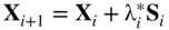
- Test the point X i+1 for optimality. If ||∇f i+1|| ≤ ε, where ε is a small quantity, take X* ≈ X i+1 and stop the process. Otherwise, go to step 5.
- Update the Hessian matrix as
(6.136)

where
(6.137)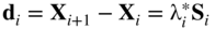 (6.138)
- Set the new iteration number as i = i + 1 and go to step 2.
Remarks
- The BFGS method can be considered as a quasi‐Newton, conjugate gradient, and variable metric method.
- Since the inverse of the Hessian matrix is approximated, the BFGS method can be called an indirect update method.
- If the step lengths
 are found accurately, the matrix, [B
i
], retains its positive definiteness as the value of i increases. However, in practical application, the matrix [B
i
] might become indefinite or even singular if
are found accurately, the matrix, [B
i
], retains its positive definiteness as the value of i increases. However, in practical application, the matrix [B
i
] might become indefinite or even singular if  are not found accurately. As such, periodical resetting of the matrix [B
i
] to the identity matrix [I] is desirable. However, numerical experience indicates that the BFGS method is less influenced by errors in
are not found accurately. As such, periodical resetting of the matrix [B
i
] to the identity matrix [I] is desirable. However, numerical experience indicates that the BFGS method is less influenced by errors in  than is the DFP method.
 - It has been shown that the BFGS method exhibits superlinear convergence near X* [19].
6.16 Test Functions
The efficiency of an optimization algorithm is studied using a set of standard functions. Several functions, involving different number of variables, representing a variety of complexities have been used as test functions. Almost all the test functions presented in the literature are nonlinear least squares; that is, each function can be represented as

where n denotes the number of variables and m indicates the number of functions (f i ) that define the least‐squares problem. The purpose of testing the functions is to show how well the algorithm works compared to other algorithms. Usually, each test function is minimized from a standard starting point. The total number of function evaluations required to find the optimum solution is usually taken as a measure of the efficiency of the algorithm. References [29–32] present a comparative study of the various unconstrained optimization techniques. Some of the commonly used test functions are given below.
- Rosenbrock's parabolic valley 8:
(6.140)


- A quadratic function:
(6.141)


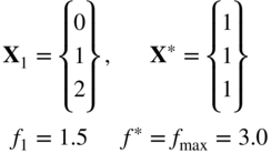
- Powell's quartic function 7:
(6.142)

- Fletcher and Powell's helical valley 21:
(6.143)

where

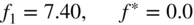
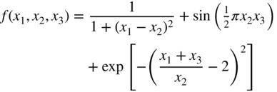
- A nonlinear function of three variables 7:
(6.144)
- Freudenstein and Roth function 27:
(6.145)


- Powell's badly scaled function 28:
(6.146)


- Brown's badly scaled function 29:
(6.147)


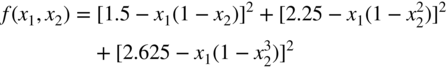
- Beale's function 29:
(6.148)

- Wood's function 30:
(6.149)


6.17 Solutions Using Matlab
The solution of different types of optimization problems using MATLAB is presented in Chapter 17. Specifically, the MATLAB solution of multivariable unconstrained optimization problem, the Rosenbrock's parabolic valley function given by Eq. (6.140), is given in Example 17.6.
References and Bibliography
- 1 Rao, S.S. (2018). The Finite Element Method in Engineering, 6e. Oxford: Elsevier‐Butterworth‐Heinemann.
- 2 Edgar, T.F. and Himmelblau, D.M. (1988). Optimization of Chemical Processes. New York: McGraw‐Hill.
- 3 Fox, R.L. (1971). Optimization Methods for Engineering Design. Reading, MA: Addison‐Wesley.
- 4 Biles, W.E. and Swain, J.J. (1980). Optimization and Industrial Experimentation. New York: Wiley.
- 5 Hicks, C.R. (1993). Fundamental Concepts in the Design of Experiments. Fort Worth, TX: Saunders College Publishing.
- 6 Hooke, R. and Jeeves, T.A. (1961). Direct search solution of numerical and statistical problems. Journal of the ACM 8 (2): 212–229.
- 7 Powell, M.J.D. (1964). An efficient method for finding the minimum of a function of several variables without calculating derivatives. The Computer Journal 7 (4): 303–307.
- 8 Rosenbrock, H.H. (1960). An automatic method for finding the greatest or least value of a function. The Computer Journal 3 (3): 175–184.
- 9 Rao, S.S. (1984). Optimization: Theory and Applications, 2e. New Delhi: Wiley Eastern.
- 10 Spendley, W., Hext, G.R., and Himsworth, F.R. (1962). Sequential application of simplex designs in optimization and evolutionary operation. Technometrics 4: 441.
- 11 Nelder, J.A. and Mead, R. (1965). A simplex method for function minimization. The Computer Journal 7: 308.
- 12 Cauchy, A.L. (1847). Méthode générale pour la résolution des systèmes d'équations simultanées. Comptes Rendus de l'Academie des Sciences , Paris 25: 536–538.
- 13 Fletcher, R. and Reeves, C.M. (1964). Function minimization by conjugate gradients. The Computer Journal 7 (2): 149–154.
- 14 Hestenes, M.R. and Stiefel, E. (1952). Methods of Conjugate Gradients for Solving Linear Systems, Report 1659, National Bureau of Standards, Washington, DC.
- 15 Marquardt, D. (1963). An algorithm for least squares estimation of nonlinear parameters. SIAM Journal on Applied Mathematics 11 (2): 431–441.
- 16 Broyden, C.G. (1967). Quasi‐Newton methods and their application to function minimization. Mathematics of Computation 21: 368.
- 17 Broyden, C.G., Dennis, J.E., and More, J.J. (1975). On the local and superlinear convergence of quasi‐Newton methods. Journal of the Institute of Mathematics and Its Applications 12: 223.
- 18 Huang, H.Y. (1970). Unified approach to quadratically convergent algorithms for function minimization. Journal of Optimization Theory and Applications 5: 405–423.
- 19 Dennis, J.E. Jr. and More, J.J. (1977). Quasi‐Newton methods, motivation and theory. SIAM Review 19 (1): 46–89.
- 20 Davidon, W.C. (1959). Variable Metric Method of Minimization, Report ANL‐5990, Argonne National Laboratory, Argonne, IL.
- 21 Fletcher, R. and Powell, M.J.D. (1963). A rapidly convergent descent method for minimization. The Computer Journal 6 (2): 163–168.
- 22 Broyden, G.G. (1970). The convergence of a class of double‐rank minimization algorithms, Parts I and II. Journal of the Institute of Mathematics and Its Applications 6, pp.: 76–90, 222–231.
- 23 Fletcher, R. (1970). A new approach to variable metric algorithms. The Computer Journal 13: 317–322.
- 24 Goldfarb, D. (1970). A family of variable metric methods derived by variational means. Mathematics of Computation 24: 23–26.
- 25 Shanno, D.F. (1970). Conditioning of quasi‐Newton methods for function minimization. Mathematics of Computation 24: 647–656.
- 26 Powell, M.J.D. (1962). An iterative method for finding stationary values of a function of several variables. The Computer Journal 5: 147–151.
- 27 Freudenstein, F. and Roth, B. (1963). Numerical solution of systems of nonlinear equations. Journal of the ACM 10 (4): 550–556.
- 28 Powell, M.J.D. (1970). A hybrid method for nonlinear equations. In: Numerical Methods for Nonlinear Algebraic Equations (ed. P. Rabinowitz), 87–114. New York: Gordon & Breach.
- 29 More, J.J., Garbow, B.S., and Hillstrom, K.E. (1981). Testing unconstrained optimization software. ACM Transactions on Mathematical Software 7 (1): 17–41.
- 30 Colville, A.R. (1968). A Comparative Study of Nonlinear Programming Codes, Report 320‐2949, IBM New York Scientific Center.
- 31 Eason, E.D. and Fenton, R.G. (1974). A comparison of numerical optimization methods for engineering design. ASME Journal of Engineering Design 96: 196–200.
- 32 Sargent, R.W.H. and Sebastian, D.J. (1972). Numerical experience with algorithms for unconstrained minimization. In: Numerical Methods for Nonlinear Optimization (ed. F.A. Lootsma), 45–113. London: Academic Press.
- 33 Shanno, D.F. (1983). Recent advances in gradient based unconstrained optimization techniques for large problems. ASME Journal of Mechanisms, Transmissions, and Automation in Design 105: 155–159.
- 34 Rao, S.S. (2017). Mechanical Vibrations, 6e. Hoboken, NJ: Pearson Education.
- 35 Haftka, R.T. and Gürdal, Z. (1992). Elements of Structural Optimization, 3e. Dordrecht, The Netherlands: Kluwer Academic.
- 36 Kowalik, J. and Osborne, M.R. (1968). Methods for Unconstrained Optimization Problems. New York: American Elsevier.
Review Questions
- 6.1 State the necessary and sufficient conditions for the unconstrained minimum of a function.
- 6.2 Give three reasons why the study of unconstrained minimization methods is important.
- 6.3 What is the major difference between zeroth‐, first‐, and second‐order methods?
- 6.4 What are the characteristics of a direct search method?
- 6.5 What is a descent method?
- 6.6
Define each term:
- Pattern directions
- Conjugate directions
- Simplex
- Gradient of a function
- Hessian matrix of a function
- 6.7 State the iterative approach used in unconstrained optimization.
- 6.8 What is quadratic convergence?
- 6.9 What is the difference between linear and superlinear convergence?
- 6.10 Define the condition number of a square matrix.
- 6.11 Why is the scaling of variables important?
- 6.12 What is the difference between random jumping and random walk methods?
- 6.13 Under what conditions are the processes of reflection, expansion, and contraction used in the simplex method?
- 6.14 When is the grid search method preferred in minimizing an unconstrained function?
- 6.15 Why is a quadratically convergent method considered to be superior for the minimization of a nonlinear function?
- 6.16 Why is Powell's method called a pattern search method?
- 6.17 What are the roles of univariate and pattern moves in the Powell's method?
- 6.18 What is univariate method?
- 6.19 Indicate a situation where a central difference formula is not as accurate as a forward difference formula.
- 6.20 Why is a central difference formula more expensive than a forward or backward difference formula in finding the gradient of a function?
- 6.21 What is the role of one‐dimensional minimization methods in solving an unconstrained minimization problem?
- 6.22 State possible convergence criteria that can be used in direct search methods.
- 6.23 Why is the steepest descent method not efficient in practice, although the directions used are the best directions?
- 6.24 What are rank 1 and rank 2 updates?
- 6.25 How are the search directions generated in the Fletcher–Reeves method?
- 6.26 Give examples of methods that require n 2, n, and 1 one‐dimensional minimizations for minimizing a quadratic in n variables.
- 6.27 What is the reason for possible divergence of Newton's method?
- 6.28 Why is a conjugate directions method preferred in solving a general nonlinear problem?
- 6.29 What is the difference between Newton and quasi‐Newton methods?
- 6.30 What is the basic difference between DFP and BFGS methods?
- 6.31 Why are the search directions reset to the steepest descent directions periodically in the DFP method?
- 6.32 What is a metric? Why is the DFP method considered as a variable metric method?
- 6.33
Answer true or false:
- A conjugate gradient method can be called a conjugate directions method.
- A conjugate directions method can be called a conjugate gradient method.
- In the DFP method, the Hessian matrix is sequentially updated directly.
- In the BFGS method, the inverse of the Hessian matrix is sequentially updated.
- The Newton method requires the inversion of an n × n matrix in each iteration.
- The DFP method requires the inversion of an n × n matrix in each iteration.
- The steepest descent directions are the best possible directions.
- The central difference formula always gives a more accurate value of the gradient than does the forward or backward difference formula.
- Powell's method is a conjugate directions method.
- The univariate method is a conjugate directions method.
Problems
- 6.1 A bar is subjected to an axial load, P
0, as shown in Figure 6.17. By using a one‐finite‐element model, the axial displacement, u(x), can be expressed as 1

where N i (x) are called the shape functions:
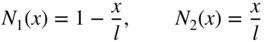
and u 1 and u 2 are the end displacements of the bar. The deflection of the bar at point Q can be found by minimizing the potential energy of the bar (f), which can be expressed as
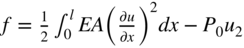
where E is Young's modulus and A is the cross‐sectional area of the bar. Formulate the optimization problem in terms of the variables u 1 and u 2 for the case P 0 l/EA = 1.
- 6.2 The natural frequencies of the tapered cantilever beam (ω) shown in Figure 6.18, based on the Rayleigh‐Ritz method, can be found by minimizing the function 34:

with respect to c 1 and c 2, where f = ω 2, E is Young's modulus, and ρ is the density. Plot the graph of 3fρl 3 /Eh 2 in (c 1, c 2) space and identify the values of ω 1 and ω 2.
- 6.3 The Rayleigh's quotient corresponding to the three‐degree‐of‐freedom spring–mass system shown in Figure 6.19 is given by 34

where

It is known that the fundamental natural frequency of vibration of the system can be found by minimizing R(X). Derive the expression of R(X) in terms of x 1, x 2, and x 3 and suggest a suitable method for minimizing the function R(X).
- 6.4 The steady‐state temperatures at points 1 and 2 of the one‐dimensional fin (x
1 and x
2) shown in Figure 6.20 correspond to the minimum of the function 1:

Plot the function f in the (x 1, x 2) space and identify the steady‐state temperatures of points 1 and 2 of the fin.
- 6.5 Figure 6.21 shows two bodies, A and B, connected by four linear springs. The springs are at their natural positions when there is no force applied to the bodies. The displacements x
1 and x
2 of the bodies under any applied force can be found by minimizing the potential energy of the system. Find the displacements of the bodies when forces of 1000 and 2000 lb are applied to bodies A and B, respectively, using Newton's method. Use the starting vector,
 .
.
Hint:

where the strain energy of a spring of stiffness k and end displacements x 1 and x 2 is given by
 k(x
2 − x
1)2 and the potential of the applied force, F
i
, is given by x
i
F
i
.
k(x
2 − x
1)2 and the potential of the applied force, F
i
, is given by x
i
F
i
. - 6.6 (a) (b) (c) (d) The potential energy of the two‐bar truss shown in Figure 6.22 under the applied load P is given by

where E is Young's modulus, A the cross‐sectional area of each member, l the span of the truss, s the length of each member, h the depth of the truss, θ the angle at which load is applied, x 1 the horizontal displacement of free node, and x 2 the vertical displacement of the free node.
- (a) Simplify the expression of f for the data E = 207 × 109 Pa, A = 10−5 m2, l = 1.5 m, h = 4 m, P = 10 000 N, and θ = 30°.
- (b)
Find the steepest descent direction, S
1, of f at the trial vector X
1 =
 .
. - (c) Derive the one‐dimensional minimization problem, f(λ), at X 1 along the direction S 1.
- (d) Find the optimal step length λ* using the calculus method and find the new design vector X 2.
- 6.7 Three carts, interconnected by springs, are subjected to the loads P
1
, P
2
, and P
3
as shown in Figure 6.23. The displacements of the carts can be found by minimizing the potential energy of the system (f):
where

Derive the function f(x 1, x 2, x 3) for the following data: k 1 = 5000 N/m, k 2 = 1500 N/m, k 3 = 2000 N/m, k 4 = 1000 N/m, k 5 = 2500 N/m, k 6 = 500 N/m, k 7 = 3000 N/m, k 8 = 3500 N/m, P 1 = 1000 N, P 2 = 2000 N, and P 3 = 3000 N. Complete one iteration of Newton's method and find the equilibrium configuration of the carts. Use X 1 = {0 0 0}T.
- 6.8
Plot the contours of the following function over the region (−5 ≤ x
1 ≤ 5, −3 ≤ x
2 ≤ 6) and identify the optimum point:

- 6.9
Plot the contours of the following function in the two dimensional (x
1, x
2) space over the region (−4 ≤ x
1 ≤ 4, −3 ≤ x
2 ≤ 6) and identify the optimum point:

- 6.10 Consider the problem

Plot the contours of f over the region (−4 ≤ x 1 ≤ 4, −3 ≤ x 2 ≤ 6) and identify the optimum point.
- 6.11 It is required to find the solution of a system of linear algebraic equations given by [A]X = b, where [A] is a known n × n symmetric positive‐definite matrix and b is an n‐component vector of known constants. Develop a scheme for solving the problem as an unconstrained minimization problem.
- 6.12
Solve the following equations using the steepest descent method (two iterations only) with the starting point, X
1 = {0 0 0}:

- 6.13
An electric power of 100 MW generated at a hydroelectric power plant is to be transmitted 400 km to a stepdown transformer for distribution at 11 kV. The power dissipated due to the resistance of conductors is i
2
c
−1, where i is the line current in amperes and c is the conductance in mhos. The resistance loss, based on the cost of power delivered, can be expressed as 0.15i
2
c
−1 dollars. The power transmitted (k) is related to the transmission line voltage at the power plant (e) by the relation
 , where e is in kilovolts. The cost of conductors is given by 2c millions of dollars, and the investment in equipment needed to accommodate the voltage e is given by 500e dollars. Find the values of e and c to minimize the total cost of transmission using Newton's method (one iteration only).
 - 6.14
Find a suitable transformation of variables to reduce the condition number of the Hessian matrix of the following function to one:

- 6.15
Find a suitable transformation or scaling of variables to reduce the condition number of the Hessian matrix of the following function to one:

- 6.16
Determine whether the following vectors serve as conjugate directions for minimizing the function
 .
.
-
- 6.17 Consider the problem:

Find the solution of this problem in the range −10 ≤ x i ≤ 10, i = 1, 2, using the random jumping method. Use a maximum of 10 000 function evaluations.
- 6.18 Consider the problem:

Find the minimum of this function in the range −5 ≤ x i ≤ 5, i = 1, 2, using the random walk method with direction exploitation.
- 6.19
Find the condition number of each matrix.
-
- 6.20 Perform two iterations of the Newton's method to minimize the function

from the starting point
 .
. - 6.21 Perform two iterations of univariate method to minimize the function given in Problem 20 from the stated starting vector.
- 6.22 Perform four iterations of Powell's method to minimize the function given in Problem 20 from the stated starting point.
- 6.23 Perform two iterations of the steepest descent method to minimize the function given in Problem 20 from the stated starting point.
- 6.24 Perform two iterations of the Fletcher–Reeves method to minimize the function given in Problem 20 from the stated starting point.
- 6.25 Perform two iterations of the DFP method to minimize the function given in Problem 20 from the stated starting vector.
- 6.26 Perform two iterations of the BFGS method to minimize the function given in Problem 20 from the indicated starting point.
- 6.27 Perform two iterations of the Marquardt's method to minimize the function given in Problem 20 from the stated starting point.
- 6.28
Prove that the search directions used in the Fletcher–Reeves method are [A]‐conjugate while minimizing the function

- 6.29 Generate a regular simplex of size 4 in a two‐dimensional space using each base point:
(a) 
(b) 
(c) 
- 6.30 Find the coordinates of the vertices of a simplex in a three‐dimensional space such that the distance between vertices is 0.3 and one vertex is given by (2, −1, −8).
- 6.31 Generate a regular simplex of size 3 in a three‐dimensional space using each base point.
(a) 
(b) 
(c) 
- 6.32 Find a vector S
2 that is conjugate to the vector
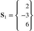
with respect to the matrix:
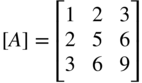
- 6.33 (a) (b) (c) (d) Compare the gradients of the function
 at
at  given by the following methods:
- (a) Analytical differentiation
- (b) Central difference method
- (c) Forward difference method
- (d) Backward difference method
Use a perturbation of 0.005 for x 1 and x 2 in the finite‐difference methods.
- 6.34 (a) (b) (c) It is required to evaluate the gradient of the function

at point
 using a finite‐difference scheme. Determine the step size Δx to be used to limit the error in any of the components, ∂f/∂x
i
, to 1% of the exact value, in the following methods:
using a finite‐difference scheme. Determine the step size Δx to be used to limit the error in any of the components, ∂f/∂x
i
, to 1% of the exact value, in the following methods:- (a) Central difference method
- (b) Forward difference method
- (c) Backward difference method
- 6.35 Consider the minimization of the function
Perform one iteration of Newton's method from the starting point
 using Eq. (6.86). How much improvement is achieved with X
2?
using Eq. (6.86). How much improvement is achieved with X
2? - 6.36 Consider the problem:

If a base simplex is defined by the vertices

find a sequence of four improved vectors using reflection, expansion, and/or contraction.
- 6.37 Consider the problem:

If a base simplex is defined by the vertices

find a sequence of four improved vectors using reflection, expansion, and/or contraction.
- 6.38 Consider the problem:

Find the solution of the problem using grid search with a step size Δx i = 0.1 in the range −3 ≤ x i ≤ 3, i = 1, 2.
- 6.39 Show that the property of quadratic convergence of conjugate directions is independent of the order in which the one‐dimensional minimizations are performed by considering the minimization of

using the conjugate directions
 and
and  and the starting point
  .
. - 6.40
Show that the optimal step length
 that minimizes f(X) along the search direction S
i
= −∇f
i
is given by Eq. (6.75).
that minimizes f(X) along the search direction S
i
= −∇f
i
is given by Eq. (6.75). - 6.41 Show that β 2 in Eq. (6.76) is given by Eq. (6.77).
- 6.42
Minimize f = 2
 +
+  from the starting point (1, 2) using the univariate method (two iterations only).
 - 6.43
Minimize
 by using the steepest descent method with the starting point (1, 2) (two iterations only).
 - 6.44
Minimize
 by the Newton's method using the starting point as (2, −1, 1).
 - 6.45
Minimize
 starting from point (0, 0) using Powell's method. Perform four iterations.
 - 6.46
Minimize
 by the simplex method. Perform two steps of reflection, expansion, and/or contraction.
 - 6.47
Solve the following system of equations using Newton's method of unconstrained minimization with the starting point
- 6.48 It is desired to solve the following set of equations using an unconstrained optimization method:

Formulate the corresponding problem and complete two iterations of optimization using the DFP method starting from
 .
. - 6.49 Solve Problem 48 using the BFGS method (two iterations only).
- 6.50 The following nonlinear equations are to be solved using an unconstrained optimization method:

Complete two one‐dimensional minimization steps using the univariate method starting from the origin.
- 6.51 Consider the two equations

Formulate the problem as an unconstrained optimization problem and complete two steps of the Fletcher–Reeves method starting from the origin.
- 6.52 Solve the equations 5x 1 + 3x 2 = 1 and 4x 1 − 7x 2 = 76 using the BFGS method with the starting point (0, 0).
- 6.53 (a) (b) (c) (d) (e) (f) (g) (h)
Indicate the number of one‐dimensional steps required for the minimization of the function
 according to each scheme:
- (a) Steepest descent method
- (b) Fletcher–Reeves method
- (c) DFP method
- (d) Newton's method
- (e) Powell's method
- (f) Random search method
- (g) BFGS method
- (h) Univariate method
- 6.54
Same as Problem 53 for the following function:

- 6.55
Verify whether the following search directions are [A]‐conjugate while minimizing the function

-
- 6.56 Solve the equations x 1 + 2x 2 + 3x 3 = 14, x 1 − x 2 + x 3 = 1, and 3x 1 − 2x 2 + x 3 = 2 using Marquardt's method of unconstrained minimization. Use the starting point X 1 = {0, 0, 0}T.
- 6.57 Apply the simplex method to minimize the function f given in Problem 20. Use the point (−1.2, 1.0) as the base point to generate an initial regular simplex of size 2 and go through three steps of reflection, expansion, and/or contraction.
- 6.58 Write a computer program to implement Powell's method using the golden section method of one‐dimensional search.
- 6.59 Write a computer program to implement the Davidon–Fletcher–Powell method using the cubic interpolation method of one‐dimensional search. Use a finite‐difference scheme to evaluate the gradient of the objective function.
- 6.60 Write a computer program to implement the BFGS method using the cubic interpolation method of one‐dimensional minimization. Use a finite‐difference scheme to evaluate the gradient of the objective function.
- 6.61 Write a computer program to implement the steepest descent method of unconstrained minimization with the direct root method of one‐dimensional search.
- 6.62 Write a computer program to implement the Marquardt method coupled with the direct root method of one‐dimensional search.
- 6.63 Find the minimum of the quadratic function given by Eq. (6.141) starting from the solution X 1 = {0, 0}T using MATLAB.
- 6.64 Find the minimum of the Powell's quartic function given by Eq. (6.142) starting from the solution X 1 = {3, −1, 0, 1}T using MATLAB.
- 6.65 Find the minimum of the Fletcher and Powell's helical valley function given by Eq. (6.143) starting from the solution X 1 = {−1, 0, 0}T using MATLAB.
- 6.66 Find the minimum of the nonlinear function given by Eq. (6.144) starting from the solution X 1 = {0, 1, 2}T using MATLAB.
- 6.67 Find the minimum of the Wood's function given by Eq. (6.149) starting from the solution X 1 = {−3, −1, −3, −1}T using MATLAB.