
The primary purpose of any network is data access. People need (or simply want) access to data that is important to them. In business settings, this may mean sales data, product data, or customer data. Whatever the case, the data must be stored somewhere. That is where database servers come in. A database server is a computer running software that allows for the storage and retrieval of data. In this chapter, we will discuss some general database basics, and then we will explore two specific database servers available for Linux.
Before we delve into the particulars of specific database implementations for Linux, it is a good idea to first explore some basics of database concepts and theory. Most readers probably have some knowledge of this area, but you may find that this section fills in a few gaps in your knowledge.
The story of databases is really the story of Structured Query Language, or SQL. SQL is the language that all relational databases use. Whether you are working with Oracle or Postgres, or even Microsoft SQL Server, that database uses SQL. The paper, “A Relational Model of Data for Large Shared Data Banks,” was published by Dr. E. F. Codd in the Association for Computing Machinery (ACM) journal, Communications of the ACM, in June 1970. While Dr. Codd wrote the paper that advanced the idea of relational databases, other researchers developed the actual SQL language.
Structured English Query Language (SEQUEL) was developed at IBM Corporation, Inc., by Donald D. Chamberlin and Raymond F. Boyce, and was specifically designed to use Codd’s model. Oracle Corp. (formally known as Relational Software) launched the first implementation of SQL for commercial distribution in 1979. Today, SEQUEL is known as SQL (pronounced “sequel”) and is accepted as the standard language for relational databases. The latest SQL standard known as SQL:99 was released in July 1999.
Data storage is not a new concept. In fact, since the earliest days of computers, how to store and retrieve data has been an issue. The method that has been dominant for many years is the relational database. This is how Microsoft SQL Server, Oracle, Postgres, and MySQL store data. Essentially, this method stores data and stores the relationships between data elements. Data is stored in units called relations. This begs the question of what, exactly, a relation is. A two-dimensional table containing data is a good example of a relation. The relation itself is the two-dimensional table, not the data contained therein. The relation includes attributes that make up that two-dimensional table; however, the actual data contained therein is particular to a given instance of the relation. There are two types of relation instances. The first type of relation instance is a table. Tables contain permanently stored data found in a relation. This is probably what most people think of when they think of storing data in a database. The second type of relation instance is the view. A view contains computed data values, rather than permanently stored data values. In other words, a view is a picture of data at a particular point. That picture could be derived from one or more tables, and it could include elements of several tables combined together.
A term that one sees often in database literature is tuple. In mathematics, a tuple is an ordered list of elements. In database terminology, a tuple is an individual record. If you are viewing a database via some graphical interface, then this will be an individual row. Another term you will see is schema. A schema is generally defined as the structure of a database—the tables, the columns for that table, etc., but not the actual data. In actuality, there are three different levels of database schema: conceptual schema, logical schema, and physical schema. The first of these, the conceptual level, emphasizes the general overview of database elements. This level defines the key features of the database, and, in some cases, will be used to establish constraints on relations. The logical level deals with the layout and relation of data elements. At this level, specific columns/attributes become important. The physical schema refers to the actual layout of the data on the storage medium. Normally, you won’t be concerned with the physical schema. Whatever database solution you are using (such as Postgres or MySQL) will handle that.
Beyond defining the relations and their attributes, a logical schema must also define the domain of those attributes. While many domains are possible, good database design requires that one utilize only those data types in standard SQL. It is a fact, however, that many database vendors add additional data types that are not SQL standard. If you utilize those data types in a database schema, then porting from one database vendor to another will be problematic. It is also important to conserve storage space. This is best accomplished by using the smallest data type that can effectively handle all possible values for a given attribute.
In order to work with SQL, you will need to know basic SQL commands. The good news is that they are relatively easy to learn. They are actually quite like English. The specific SQL commands SELECT, FROM, and WHERE are given in capital letters so they stand out. Now this book is about network administration, but if your duties include administering a database server, then you must have a basic understanding of SQL. In this section, we will cover the basics of SQL. The basic syntax of an SQL query looks like this:
SELECT column_name(s) FROM table_name
If, rather than selecting a specific column or columns, you want all columns, then you can use the asterisk (*) to denote that:
SELECT * FROM table_name
An example might look like this:
SELECT LastName,FirstName FROM Employees
However, these examples get you all the records from that table, or at least (as in the last example) certain columns from every record in the database. This is where the WHERE clause comes in. It essentially says to only get records if some criteria is met. It looks like this:
SELECT column_name(s) FROM table_name WHERE column_name operator value
Here is a specific example:
SELECT * FROM Employees WHERE City='Dallas'
While this is very simple, it is the essence of the SQL query: simply selecting records based on some criteria.
Now this example introduces you to the WHERE clause, but also to the = operator. That is only one operator you can use with the WHERE clause. There are others:
= Equal
! Not equal
> Greater than
< Less than
>= Greater than or equal
<= Less than or equal
BETWEENBetween an inclusive rangeLIKESearch for a pattern
The first few work much like the = sign. If you want to use !, >, <=, and so on, they work much like the = symbol. You might have an example like this:
SELECT * FROM Employees WHERE AGE > 21
But the LIKE qualifier is a bit different. The LIKE statement enables you to get back records that are similar to the criteria you put in. Here is an example:
SELECT * FROM Employees WHERE LastName LIKE 'B%'
The % symbol is a wild card. This statement is saying “get all the records in the employees table where the last name starts with a B.” That means Brown, Benson, Bartholomew, etc. The LIKE keyword is pretty useful.
There are also cases where you may have more than one criteria. In these cases, you will want to use a modifier with your SELECT statement.
The AND operator displays a record if both the first condition and the second condition are true.
The OR operator displays a record if either the first condition or the second condition is true.
SELECT * FROM Employees WHERE City='Chicago' AND LastName='Johnson'
SELECT * FROM Employees WHERE City='San Francisco' OR City='New York'
Although our examples only show one AND and one OR, you can chain together as many of these as needed to create the database logic your search requires.
Another important keyword is DISTINCT. This keyword is telling the database to ignore duplicate records. The basic syntax is like this:
SELECT DISTINCT column_name(s) FROM table_name
If, for example, you wanted a list of cities found in your Employees table, but wanted to omit duplicates, then this code would work like this:
SELECT DISTINCT City FROM Employees
The ORDER BY clause is used to sort the data retrieved. You simply select what column you want to use to sort the records. The general syntax is like this:
SELECT column_name(s) FROM table_name ORDER BY column_name(s) ASC|DESC
A specific example would be:
SELECT * FROM Employees ORDER BY LastName
The BETWEEN operator selects a range of data between two values. The general syntax is:
SELECT column_name(s) FROM table_name WHERE column_name BETWEEN value1 AND value2
A specific example would be:
SELECT * FROM Employees
WHERE LastName
BETWEEN 'Jones' AND 'McMurray'
These basic select options are enough to allow you to perform a wide range of queries on any given database. The SELECT statement and the various modifiers we have just explored are the most commonly used SQL statements.
In addition to these query options, SQL offers a number of mathematical functions you may find useful. Here are some of the most commonly used. You should notice that some of these (like AVG, SUM, etc.) require that the column being used contain a mathematical data type, such as an integer. Using a string as the argument to these functions will not work. However, others, like COUNT, can take any data type as an argument.
The AVG function returns the mathematical mean for a given column. Its general syntax is:
SELECT AVG(column_name) FROM table_name
A specific example would be:
SELECT AVG(Salary) FROM Employees
The COUNT function literally counts the number of entries and returns that value. The general syntax is:
SELECT COUNT(column_name) FROM table_name
A specific example would look like this:
SELECT COUNT(LastName) FROM Employees
The FIRST function returns the very first entry in the table for that column. The general syntax looks like this.
SELECT FIRST(column_name) FROM table_name
A specific example would look like this:
SELECT FIRST(LastName) FROM Employees
The LAST function does the exact opposite of the FIRST function and has the same syntax.
The MAX function returns the maximum value found in that particular column. The minimum does the exact opposite. The general syntax looks like this.
SELECT MAX(column_name) FROM table_name
Here is a specific example:
SELECT MAX(Salary) FROM Employees
The SUM function adds up all the values for a given column and returns the sum. Here is the basic syntax.
SELECT SUM(column_name) FROM table_name
A specific example might look like this:
SELECT SUM(Salary) FROM Employees
So far all the examples we have looked at retrieved data from just one table, but it is not at all uncommon to need records from more than one table. That brings us to the join commands. While there are several types of joins, the most basic is the inner join. Here is the basic syntax:
SELECT column_name(s) FROM table_name1 INNER JOIN table_name2 ON table_name1.column_name=
table_name2.column_name
Here is a more specific example:
SELECT Employees.LastName, Employees.FirstName, Orders.OrderNo FROM Employees INNER
JOIN Orders ON Employees.P_Id=Orders.P_Id ORDER BY Employees.LastName
What this statement is saying is to get certain columns from the Employees table and also to get certain records from the Orders table. It joins them where Employees.P_Id equals Orders.P_Id. This is the most basic type of join.
Now in this section, we have not covered all the various nuances of SQL; however, we have gone over the basics, and you should be able to write simple SQL queries effectively.
In this section, we will touch on a few more advanced SQL commands. Some of the SQL discussed here is more complex than the previous SQL commands. Other commands are not any more complex, just less commonly used. These commands should be more than enough SQL knowledge for you to accomplish your duties as a network administrator.
The LIMIT command enables you to retrieve rows within a specified range. The LIMIT count determines the number of rows returned; however, this command may return fewer rows than designated if the query itself yields fewer rows.
SELECT * FROM mytable LIMIT 5
This command basically states that you want all the columns in mytable, but only shows the first five records returned.
This command checks if a value is NULL and allows you to return a different value if it is. The format is as follows:
ISNULL(check-expression,replace-expression)
SELECT Description, ISNULL(Qty, 0.00) AS 'Max Quantity' FROM Sales;
You can create, change, or even delete entire tables with SQL commands. These commands may be more important to a network administrator than the queries we covered previously in this chapter. The reason is that it is much more likely that a network administrator will be creating databases or tables, rather than retrieving data from them.
First, creating an entire database is quite easy. Here is the basic syntax:
CREATE DATABASE database_name
Here is an example:
CREATE DATABASE my_db
Creating a table is just a little more complicated. You have to identify the column names and data types. Here is the basic syntax:
CREATE TABLE table_name ( column_name1 data_type, column_name2 data_type,
 column_ name3 data_type, .... )
Now let’s look at an actual example:
CREATE TABLE Employees
( P_Id int,
LastName varchar(255),
FirstName varchar(255),
Address varchar(255),
City varchar(255) )
The ALTER TABLE statement is used to add, drop, or modify columns in an existing table. The basic syntax looks like this:
ALTER TABLE table_name ADD column_name datatype
ALTER TABLE table_name DROP COLUMN column_name
ALTER TABLE table_name ALTER COLUMN column_name datatype
Here are some examples:
ALTER TABLE Employees ADD DateOfHire date
ALTER TABLE Employees DROP COLUMN DateOfHire
The SQL UNION operator combines the results of two or more SELECT statements. Here is the basic syntax:
SELECT column_name(s) FROM table_name1 UNION SELECT column_name(s) FROM table_name2
SELECT LastName FROM Employees
UNION
SELECT LastName FROM Customers
The SELECT INTO statement retrieves data from one table and inserts it into another table. Here is the basic syntax:
SELECT * INTO new_table_name [IN externaldatabase] FROM old_table_name
Here is an example:
SELECT * INTO Employees_Backup FROM Employees
Database administrators utilize triggers to establish relationships among different databases. For example, when new records are added to one table, new records are subsequently added to related tables. Triggers are essentially stored procedures that automatically execute in response to certain events. Associated with a specific table, a trigger is configured to execute when records are modified (inserted, updated, or deleted). We will see how to create triggers when we examine Postgres Admin.
The entire purpose of relational databases is to keep data in a format that relates various items to other items. For example, you have a table of employees and another table of job descriptions. By relating the two tables, you can easily retrieve the job description for any employee. One of the goals of relational databases is to reduce or eliminate duplication. The process of reducing duplication in the data is called database normalization. Or to put it more formally, database normalization is the process of removing, or at least reducing, anomalies in a database. Anomalies occur due to data redundancy existing in the database relations, due to poor design. The fundamental anomaly of data redundancy leads to two additional anomalies: update and deletion anomalies. Update anomalies occur when the data in one record is updated, but the related data existing in another record is not. Deletion anomalies occur when data in one record is deleted, but the related data in another record is not. In both cases, the anomalies are due to the initial data redundancy.
Therefore, normalization is, ultimately, the process of removing redundancies. There are multiple levels of normalization. E. F. Codd initially introduced what is now known as 1N normalization. In 1N normalization, there are no duplicate records, but there may be duplicated columns. Furthermore, each relation has a unique key. Later, Codd introduced 2N normalization. 2N normalization adds the requirement of functional dependencies based on keys. For example, a table that had a foreign key linking it to another table would satisfy this aspect of 2N normalization.
In 1971, 3N normalization was introduced by Codd. In 3N normalization, any column that is not dependent upon the primary key is removed from the relation. Obviously, this level of normalization can lead to more complex joins when querying the data. And frankly higher levels of normalization might not always be desirable. One must balance between the level of normalization desired and the speed and efficiency of queries. There are levels of normalization beyond 3N, but it is not common to take database normalization beyond 3N for most business needs.
By now, you should have a good understanding of how relational databases work, basic SQL, and even database normalization. It is time for us to explore specific database implementation. In the world of Linux, there are two database management engines that are dominant: MySQL and Postgres.
MySQL is an open source database. You can get it from www.MySQL.org. It has become very popular in the Linux community. In fact, you will frequently encounter the term LAMP development. This means Linux operating system, Apache Web server, MySQL database, and Perl/PHP/Python used for programming.
Using most Linux desktops, you can install MySQL from the desktop. For example, in Debian, it is as simple as checking the boxes next to the MySQL packages (see Figure 18.1).
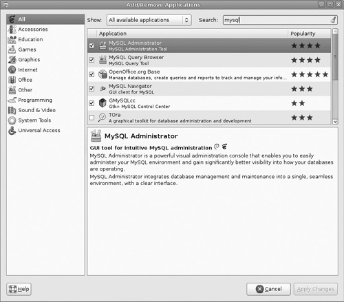
Note that the MySQL administrator is a graphical user interface tool you will definitely want to have. However, this only installs the MySQL add-on utilities. To install MySQL and to set the initial configuration, you are going to need some basic shell commands.
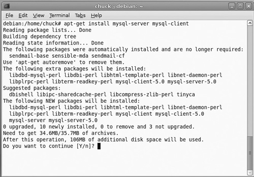
sudo apt-get install mysql-server mysql-client
Note that some Web resources have a similar shell command but include a specific version number. Don’t use those examples. The problem is that if the specific version number is no longer current, you will get an error. If you use the method I just showed you, it will install the latest version (see Figure 18.2).
The installation process will prompt you to set a password for administering this in MySQL server (see Figure 18.3).
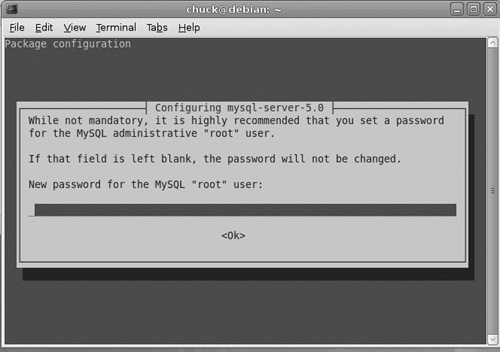
If you don’t set the password during installation, it is easily accomplished from the shell:
sudo mysqladmin -u root -h localhost password 'mypassword'
sudo mysqladmin -u root -h myhostname password 'mypassword'
You are now ready to use MySQL. You can access it from the shell with the following login:
mysql -u root -p <password>
Now you can certainly work with MySQL from the shell, but given the complexities involved, particularly with SQL statements, I strongly recommend that you do this from a GUI. In this case, there is an excellent one called MySQL Administrator.
In this section, we will provide you with a brief tutorial of the basic functions in MySQL Administrator, along with screenshots where appropriate. It should be noted that this is just a brief tutorial designed to assist the MySQL novice in getting started. If you intend to work with MySQL on a professional level, at a minimum, you should carefully study all documentation available at www.mysql.org. You may also consider reviewing the help file that comes with MySQL Administrator.
When you first launch the administrator, you will be prompted to log in (see Figure 18.4).
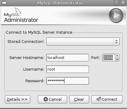
This will take you to the main screen (see Figure 18.5), which begins with a summary of the server status, including the version of MySQL currently running.
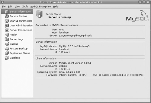
You also have a number of options on the left-hand side, which are used to manage this MySQL server. We will look briefly at each of these.
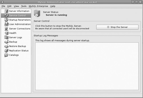
The first option, Service Control (see Figure 18.6), is the easiest. It simply allows you to stop or start the service, and it provides you with any log messages from the service startup.
The next option, Startup Parameters, is considerably more complex (see Figure 18.7), but don’t worry. You can leave all these settings with their default values. In fact, unless you have a compelling reason to do otherwise, you should leave them with default values.
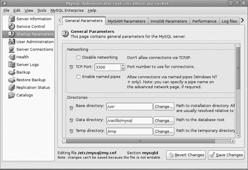
Frankly, the first tab should absolutely be left with default settings. Changing the port you use or the directories for critical files can render your database server unusable.
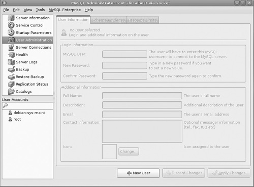
The User Administration screen comes next (see Figure 18.8). This will allow you to add or edit users. This screen is very easy to follow.
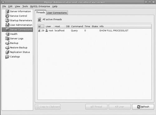
The next screen may be the simplest of all. It simply shows you current threads running and any current user connections (see Figure 18.9).
This brings us to the Server Health screen (see Figure 18.10).
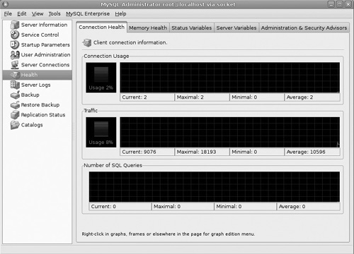
This may be one of the most critical screens. The first few tabs give you information on CPU and memory usage, as well as statistics such as uptime. The Server Variables tab allows you to view a host of server variables, including the default character set and the port. The final tab, Administration & Security Advisors, gives you tips on securing your MySQL installation.
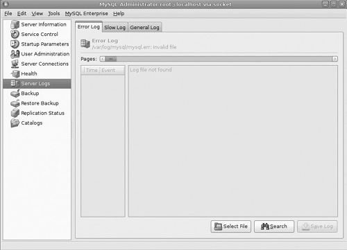
The Server Logs tab provides a very easy and convenient way for you to view the MySQL Server Logs (see Figure 18.11).
The Backup and Restore Backup options provide a very convenient and user-friendly way to create database backups and to restore them (see Figure 18.12).
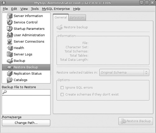
There are a number of backup options you can set; you can even schedule the backup to occur at specific times. It is critical that your database be backed up frequently. How frequently is dependent on your environment. For example, a high school might only need to back up once per day. But an ecommerce site might get backed up every hour.
The other two options on the left are not critical for you at this point. For example, Replication Status lets you know the status of replicating your server with another server. In situations where high availability is critical, it is common practice to replicate a server so there is a backup server running and ready to go if there is a problem. While this is an important issue, it is really beyond the scope of our basic introduction to MySQL.
Postgres is another option for databases in Linux. You can get Postgres, as well as view documentation, at www.postgresql.org/. Postgres began as a project at the Defense Advanced Research Project Agency (DARPA) and is now a widely used open source database solution.
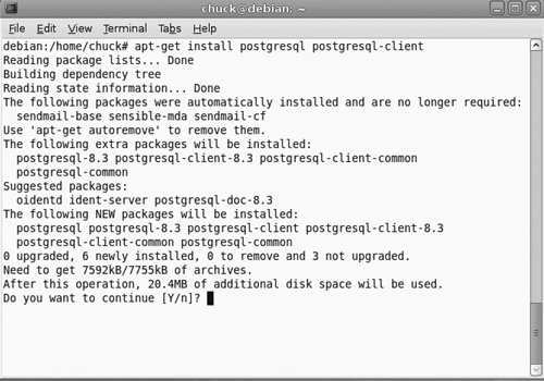
Installing Postgres is easy (see Figure 18.13). Just type in as root:
apt-get install postgresql postgresql-client
Now, just like MySQL, you can configure and work with Postgres from the command line, but I don’t recommend it.
For those who insist on working with Postgres via shell commands, let’s look at a few basic commands
To access a database, use:
psql mydatabasename
If you leave off the database name, then it will default to your user account name and your default database. When using psql, you will be greeted with the following message:
Welcome to psql 9.0.1 (or whatever your version number is)
Postgres expects you to use the SELECT command (just like with SQL), even to get information about Postgres, for example:
SELECT version();
SELECT current_date;
To exit psql, just type:
q
You can create a user with this command:
createuser chuck --pwprompt
To access a specific database as a specific user:
psql -U chuck -W mytestdb
Beyond these commands, you can execute SQL statements right at the shell. For more details, go to www.postgresql.org/docs/9.0/interactive/index.html.
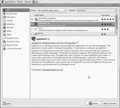
Fortunately, it also has a nice, easy-to-use GUI, called pgAdmin. You can install it by using the Add/Remove programs portion of your desktop (see Figure 18.14).
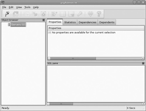
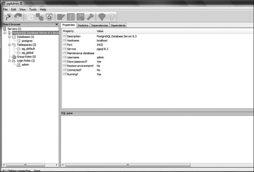
The pgAdmin screen is laid out a bit differently than MySQL Admin, but it has many similar functions (see Figure 18.15).
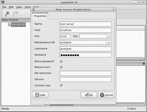
To create a new database, you first create a new server. You start by selecting File > Add Server (see Figure 18.16) and simply fill in the details.
Note that it is not uncommon for people to experience issues at this point. Those issues will be specific to your Linux distribution, so if you experience any you will need to refer to your distributions documentation. For example, Debian frequently has a permissions issue at this point.
After you have connected to a database (or created a new one), your pgAdmin screen will display elements of that database (see Figure 18.17).
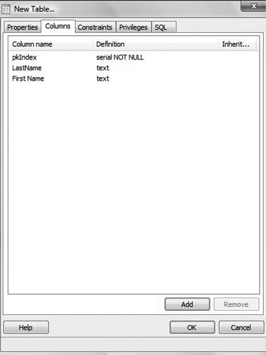
Creating a new table (or any other element of a database) is a very easy matter in pgAdmin. You simply choose a new table and fill in the data (see Figure 18.18).
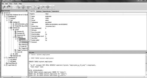
You can also expand any server to see its databases, and you can expand the database to see its tables, triggers, functions, and all its elements (see Figure 18.19).
pgAdmin makes administering your Postgres database remarkably easy. I recommend you spend a little time familiarizing yourself with this tool. As you have already seen, much of it is self-explanatory.
Note that Postgres does not support all the standard SQL commands. Whether you are using the shell commands or pgAdmin, there are several functions that Postgres does not support, which are listed here:
mid()len()round()format()first()top ()ifnull()
In this chapter, you have been given the essentials of database theory and design. We have also explored the basics of structure query language and showed you how to install, configure, and use MySQL and Postgres. You should be able to install and configure a database server for your network and to administer that server. Given the ubiquitous and critical nature of databases, I would highly recommend that you make certain you fully understand this chapter before proceeding. You may even need to read it more than once.