
In This Chapter
This chapter provides an overview of Excel’s formula-related features and describes some techniques that might be new to you.
An overview of Excel formulas
Differentiating between absolute and relative references in formulas
Understanding and using names
Introducing array formulas
Counting and summing cells
Working with dates and times
Creating megaformulas
Virtually every successful spreadsheet application uses formulas. In fact, constructing formulas can certainly be construed as a type of programming.
Note

For a much more comprehensive treatment of Excel formulas and functions, refer to my book, Excel 2007 Formulas (Wiley).
Formulas, of course, are what make a spreadsheet a spreadsheet. If it weren’t for formulas, your worksheet would just be a static document — something that could be produced by a word processor that has great support for tables.
Excel has a huge assortment of built-in functions, has excellent support for names, and even supports array formulas (a special type of formula that can perform otherwise impossible calculations).
A formula entered into a cell can consist of any of the following elements:
Operators such as + (for addition) and * (for multiplication)
Cell references (including named cells and ranges)
Numbers or text strings
Worksheet functions (such as SUM or AVERAGE)
A formula in Excel 2007 can consist of up to 8,000 characters. After you enter a formula into a cell, the cell displays the result of the formula. The formula itself appears in the formula bar when the cell is activated.
You’ve probably noticed that the formulas in your worksheet get calculated immediately. If you change a cell that a formula uses, the formula displays a new result with no effort on your part. This is what happens when the Excel Calculation mode is set to Automatic. In this mode (which is the default mode), Excel uses the following rules when calculating your worksheet:
When you make a change — enter or edit data or formulas, for example — Excel immediately calculates those formulas that depend on the new or edited data.
If it’s in the middle of a lengthy calculation, Excel temporarily suspends calculation when you need to perform other worksheet tasks; it resumes when you’re finished.
Formulas are evaluated in a natural sequence. In other words, if a formula in cell D12 depends on the result of a formula in cell D11, cell D11 is calculated before D12.
Sometimes, however, you might want to control when Excel calculates formulas. For example, if you create a worksheet with thousands of complex formulas, operations can slow to a snail’s pace while Excel does its thing. In such a case, you should set Excel’s calculation mode to Manual. Use the Calculation Options control in the Formulas ![]() Calculation group.
Calculation group.
When you’re working in Manual Calculation mode, Excel displays Calculate in the status bar when you have any uncalculated formulas. You can press the following shortcut keys to recalculate the formulas:
F9 calculates the formulas in all open workbooks.
Shift+F9 calculates the formulas in the active worksheet only. Other worksheets in the same workbook won’t be calculated.
Ctrl+Alt+F9 forces a recalculation of everything in all workbooks. Use it if Excel (for some reason) doesn’t seem to be calculating correctly, or if you want to force a recalculation of formulas that use custom functions created with Visual Basic for Applications (VBA).
Ctrl+Alt+Shift+F9 rechecks all dependent formulas, and calculates all cells in all workbooks (including cells not marked as needing to be calculated).
Most formulas reference one or more cells. This reference can be made by using the cell’s or range’s address or name (if it has one). Cell references come in four styles:
Relative: The reference is fully relative. When the formula is copied, the cell reference adjusts to its new location. Example: A1.
Absolute: The reference is fully absolute. When the formula is copied, the cell reference does not change. Example: $A$1.
Row Absolute: The reference is partially absolute. When the formula is copied, the column part adjusts, but the row part does not change. Example: A$1.
Column Absolute: The reference is partially absolute. When the formula is copied, the row part adjusts, but the column part does not change. Example: $A1.
By default, all cell and range references are relative. To change a reference, you must manually add the dollar signs. Or, when editing a cell in the formula bar, move the cursor to a cell address and press F4 repeatedly to cycle through all four types of cell referencing.
If you think about it, you’ll realize that the only reason why you would ever need to change a reference is if you plan to copy the formula. Figure 3-1 demonstrates why this is so. The formula in cell C3 is
=$B3*C$2
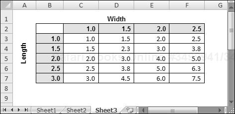
This formula calculates the area for various lengths (listed in column B) and widths (listed in row 3). After the formula is entered, it can then be copied down to C7 and across to F7. Because the formula uses absolute references to row 2 and column B and relative references for other rows and columns, each copied formula produces the correct result. If the formula used only relative references, copying the formula would cause all the references to adjust and thus produce incorrect results.
Normally, Excel uses what’s known as A1 notation: Each cell address consists of a column letter and a row number. However, Excel also supports R1C1 notation. In this system, cell A1 is referred to as cell R1C1, cell A2 as R2C1, and so on.
To change to R1C1 notation, access the Formulas tab of the Excel Options dialog box. Place a check mark next to R1C1 Reference Style. After you do so, you’ll notice that the column letters all change to numbers. All the cell and range references in your formulas are also adjusted.
Table 3-1 presents some examples of formulas that use standard notation and R1C1 notation. The formula is assumed to be in cell B1 (also known as R1C2).
If you find R1C1 notation confusing, you’re not alone. R1C1 notation isn’t too bad when you’re dealing with absolute references. But when relative references are involved, the brackets can be very confusing.
The numbers in brackets refer to the relative position of the references. For example, R[–5]C[–3] specifies the cell that’s five rows above and three columns to the left. On the other hand, R[5]C[3] references the cell that’s five rows below and three columns to the right. If the brackets are omitted, the notation specifies the same row or column. For example, R[5]C refers to the cell five rows below in the same column.
Although you probably won’t use R1C1 notation as your standard system, it does have at least one good use. Using R1C1 notation makes it very easy to spot an erroneous formula. When you copy a formula, every copied formula is exactly the same in R1C1 notation. This is true regardless of the types of cell references that you use (relative, absolute, or mixed). Therefore, you can switch to R1C1 notation and check your copied formulas. If one looks different from its surrounding formulas, there’s a good chance that it might be incorrect.
In addition, if you write VBA code to create worksheet formulas, you might find it easier to create the formulas by using R1C1 notation.
When a formula refers to other cells, the references need not be on the same sheet as the formula. To refer to a cell in a different worksheet, precede the cell reference with the sheet name followed by an exclamation point. Here’s an example of a formula that uses a cell reference in a different worksheet (Sheet2):
=Sheet2!A1+1
You can also create link formulas that refer to a cell in a different workbook. To do so, precede the cell reference with the workbook name (in square brackets), the worksheet name, and an exclamation point. Here’s an example:
=[Budget.xlsx]Sheet1!A1
If the workbook name in the reference includes one or more spaces, you must enclose it (and the sheet name) in single quotation marks. For example:
='[Budget For 2008.xlsx]Sheet1'!A1
Referencing Data in a Table
Excel 2007 supports a special type of range that has been designated as a table (using the Insert ![]() Tables
Tables ![]() Table command). Tables add a few new twists to formulas.
Table command). Tables add a few new twists to formulas.
When you enter a formula into a cell in a table, Excel automatically copies the formula to all of the other cells in the column — but only if the column was empty. This is known as a calculated column. If you add a new row to the table, the calculated column formula is entered automatically for the new row. Most of the time, this is exactly what you want. If you don’t like the idea of Excel entering formulas for you, use the SmartTag to turn this feature off. The SmartTag appears after Excel enters the calculated column formula.
Excel 2007 also supports “structured referencing” for referring to cells within a table. The table in the accompanying figure is named Table1.
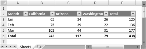
You can create formulas that refer to cells within the table by using the column headers. In some cases, this may make your formulas easier to understand. But the real advantage is that your formulas will continue to be valid if rows are added or removed from the table. For example, these are all valid formulas:
=SUM(Table1[Washington])
=Table1[[#Totals],[California]]
=Table1[[#Headers],[California]]
=SUM(Table1[[#This Row],[California]:[Washington]])
The last formula, which uses [#This Row], is valid only if it’s in a cell in one of the rows occupied by the table.
If the linked workbook is closed, you must add the complete path to the workbook reference. Here’s an example:
='C:BudgetingExcel Files[Budget For 2008.xlsx]Sheet1'!A1
Although you can enter link formulas directly, you can also create the reference by using normal pointing methods. To do so, the source file must be open. When you do so, Excel creates absolute cell references. If you plan to copy the formula to other cells, make the references relative.
Working with links can be tricky. For example, if you choose the Office ![]() Save As command to make a backup copy of the source workbook, you automatically change the link formulas to refer to the new file (not usually what you want to do). Another way to mess up your links is to rename the source workbook when the dependent workbook is not open.
Save As command to make a backup copy of the source workbook, you automatically change the link formulas to refer to the new file (not usually what you want to do). Another way to mess up your links is to rename the source workbook when the dependent workbook is not open.
One of the most useful features in Excel is its ability to provide meaningful names for various items. For example, you can name cells, ranges, rows, columns, charts, and other objects. You can even name values or formulas that don’t appear in cells in your worksheet (see the “Naming constants” section, later in this chapter).
Excel provides several ways to name a cell or range:
Choose Formulas
 Named Cells Name a Range to display the New Name dialog box.
Use the Name Manager dialog box (Formulas
Defined Names Name Manager or press Ctrl+F3). This is not the most efficient method because it requires clicking the New button in the Name Manger dialog box, which displays the New Name dialog box.Select the cell or range and then type a name in the Name box and press Enter. The Name box is the drop-down control displayed to the left of the formula bar.
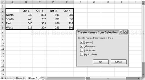
If your worksheet contains text that you would like to use for names of adjacent cells or ranges, select the text and the cells to be named and choose Formulas
Defined Names Create from Selection. In Figure 3-2, for example, B3:E3 is named North, B4:E4 is named South, and so on. Vertically, B3:B6 is named Qtr1, C3:C6 is named Qtr2, and so on.
Using names is especially important if you write VBA code that uses cell or range references. The reason? VBA does not automatically update its references if you move a cell or range that’s referred to in a VBA statement. For example, if your VBA code writes a value to Range(“C4”), the data will be written to the wrong cell if the user inserts a new row above or a new column to the left of cell C4. Using a reference to a named cell, such as Range(“InterestRate”), avoids these potential problems.
When you create a name for a cell or a range, Excel doesn’t automatically use the name in place of existing references in your formulas. For example, assume that you have the following formula in cell F10:
=A1-A2
If you define the names Income for A1 and Expenses for A2, Excel will not automatically change your formula to
=Income-Expenses
However, it’s fairly easy to replace cell or range references with their corresponding names. Start by selecting the range that contains the formulas that you want to modify. Then choose the Formulas ![]() Defined Names
Defined Names ![]() Name a Range
Name a Range ![]() Apply Names. In the Apply Names dialog box, select the names that you want to apply and then click OK. Excel replaces the range references with the names in the selected cells.
Apply Names. In the Apply Names dialog box, select the names that you want to apply and then click OK. Excel replaces the range references with the names in the selected cells.
Note
Unfortunately, there is no way to automatically unapply names. In other words, if a formula uses a name, you can’t convert the name to an actual cell or range reference. Even worse, if you delete a name that is used in a formula, the formula does not revert to the cell or range address — it simply returns a #NAME? error.
My Power Utility Pak add-in (available at a discount by using the coupon in the back of the book) includes a utility that scans all formulas in a selection and automatically replaces names with their cell addresses.
Excel has a special operator called the intersection operator that comes into play when you’re dealing with ranges. This operator is a space character. Using names with the intersection operator makes it very easy to create meaningful formulas. For this example, refer to Figure 3-2. If you enter the following formula into a cell
=Qtr_2 South
the result is 732 — the intersection of the Qtr2 range and the South range.
Excel lets you name complete rows and columns. In the preceding example, the name Qtr1 is assigned to the range B3:B6. Alternatively, Qtr1 could be assigned to all of column B, Qtr2 to column C, and so on. You also can do the same horizontally so that North refers to row 3, South to row 4, and so on.
The intersection operator works exactly as before, but now you can add more regions or quarters without having to change the existing names.
When naming columns and rows, make sure that you don’t store any extraneous information in named rows or columns. For example, remember that if you insert a value in cell C7, it is included in the Qtr1 range.
A named cell or range normally has a workbook-level scope. In other words, you can use the name in any worksheet in the workbook.
Another option is to create names that have a worksheet-level scope. To create a worksheet-level name, define the name by preceding it with the worksheet name followed by an exclamation point: for example, Sheet1!Sales. If the name is used on the sheet in which it is designed, you can omit the sheet qualifier when you reference the name. You can, however, reference a worksheet-level name on a different sheet if you precede the name with the sheet qualifier.
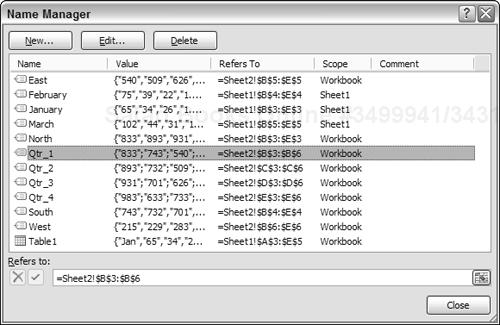
The Name Manager dialog box (Formulas ![]() Defined Names
Defined Names ![]() Name Manager) makes it easy to identify names by their scope (see Figure 3-3). Note that you can sort the names within this dialog box. For example, click the Scope column header, and the names are sorted by scope.
Name Manager) makes it easy to identify names by their scope (see Figure 3-3). Note that you can sort the names within this dialog box. For example, click the Scope column header, and the names are sorted by scope.
Virtually every experienced Excel user knows how to create cell and range names (although not all Excel users actually do so). But most Excel users do not know that you can use names to refer to values that don’t appear in your worksheet — that is, constants.
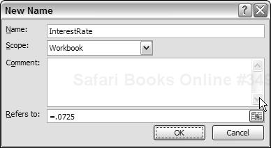
Suppose that many formulas in your worksheet need to use a particular interest rate value. One approach is to type the interest rate into a cell and give that cell a name, such as InterestRate. After doing so, you can use that name in your formulas, like this:
=InterestRate*A3
An alternative is to call up the New Name dialog box (Formulas ![]() Defined Names
Defined Names ![]() Define Name) and enter the interest rate directly into the Refers To box (see Figure 3-4). Then you can use the name in your formulas just as if the value were stored in a cell. If the interest rate changes, just change the definition for InterestRate, and Excel updates all the cells that contain this name.
Define Name) and enter the interest rate directly into the Refers To box (see Figure 3-4). Then you can use the name in your formulas just as if the value were stored in a cell. If the interest rate changes, just change the definition for InterestRate, and Excel updates all the cells that contain this name.
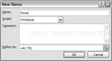
In addition to naming cells, ranges, and constants, you can also create named formulas. To do so, enter a formula directly into the Refers To field in the New Name dialog box.
This is a very important point: The formula that you enter uses cell references relative to the active cell at the time that you create the named formula.
Figure 3-5 shows a formula (=A1^B1) entered directly in the Refers To box in the New Name dialog box. In this case, the active cell is C1, so the formula refers to the two cells to its left. (Notice that the cell references are relative.) After this name is defined, entering =Power into a cell raises the value two cells to the left to the power represented by the cell directly to the left. For example, if B10 contains 3 and C10 contains 4, entering the following formula into cell D10 returns a value of 81 (3 to the 4th power):
=Power
When you display the New Name dialog box after creating the named formula, the Refers To box displays a formula that is relative to the current active cell. For example, if cell D32 is the active cell, the Refers To box displays
=Sheet1!B32^Sheet1!C32
Notice that Excel appends the worksheet name to the cell references used in your formula. This, of course, will cause the named formula to produce incorrect results if you use it on a worksheet other than the one in which it was defined. If you would like to use this named formula on a sheet other than Sheet1, you need to remove the sheet references from the formula (but keep the exclamation points). For example:
=!A1^!B1
After you understand the concept, you might discover some new uses for named formulas. One distinct advantage is apparent if you need to modify the formula. You can just change the formula one time rather than edit each occurrence of the formula.
In addition to providing names for cells and ranges, you can give more meaningful names to objects such as pivot tables and shapes. This can make it easier to refer to such objects, especially when you refer to them in your VBA code.
To change the name of a nonrange object, use the Name box, which is located to the left of the formula bar. Just select the object, type the new name in the Name box, and then press Enter.
Note
If you simply click elsewhere in your workbook after typing the name in the Name box, the name won’t stick. You must press Enter.
For some reason, Excel 2007 does not allow you to use the Name box to rename a chart. You must use Chart Tools ![]() Layout
Layout ![]() Properties
Properties ![]() Chart Name.
Chart Name.
It’s not uncommon to enter a formula and receive an error in return. One possibility is that the formula you entered is the cause of the error. Another possibility is that the formula refers to a cell that has an error value. The latter scenario is known as the ripple effect — a single error value can make its way to lots of other cells that contain formulas that depend on the cell. The tools in the Formulas ![]() Formula Auditing group can help you trace the source of formula errors.
Formula Auditing group can help you trace the source of formula errors.
Table 3-2 lists the types of error values that may appear in a cell that has a formula.
Table 3-2. Excel Error Values
Error Value | Explanation |
|---|---|
#DIV/0! | The formula is trying to divide by 0 (zero) (an operation that’s not allowed on this planet). This error also occurs when the formula attempts to divide by a cell that is empty. |
#N/A | The formula is referring (directly or indirectly) to a cell that uses the NA worksheet function to signal the fact that data is not available. A LOOKUP function that can’t locate a value also returns #N/A. |
#NAME? | The formula uses a name that Excel doesn’t recognize. This can happen if you delete a name that’s used in the formula or if you have unmatched quotes when using text. A formula will also display this error if it uses a function defined in an add-in and that add-in is not installed. |
#NULL! | The formula uses an intersection of two ranges that don’t intersect. (This concept is described earlier in the chapter.) |
#NUM! | There is a problem with a function argument; for example, the SQRT function is attempting to calculate the square root of a negative number. This error also appears if a calculated value is too large or small. Excel does not support non-zero values less than 1E–307 or greater than 1E+308 in absolute value. |
#REF! | The formula refers to a cell that isn’t valid. This can happen if that cell has been deleted from the worksheet. |
#VALUE! | The formula includes an argument or operand of the wrong type. An operand is a value or cell reference that a formula uses to calculate a result. This error also occurs if your formula uses a custom VBA worksheet function that contains an error. |
##### | A cell displays a series of hash marks under two conditions: the column is not wide enough to display the result, or the formula returns a negative date or time value. |
In Excel terminology, an array is a collection of cells or values that is operated on as a group. An array formula is a special type of formula that works with arrays. An array formula can produce a single result, or it can produce multiple results — with each result displayed in a separate cell.
For example, when you multiply a 1 x 5 array by another 1 x 5 array, the result is a third 1 x 5 array. In other words, the result of this kind of operation occupies five cells; each element in the first array is multiplied by each corresponding element in the second array to create five new values, each getting its own cell. The array formula that follows multiplies the values in A1:A5 by the corresponding values in B1:B5. This array formula is entered into five cells simultaneously:
{=A1:A5*B1:B5}Note
You enter an array formula by pressing Ctrl+Shift+Enter. To remind you that a formula is an array formula, Excel surrounds it with curly braces in the formula bar. When I present an array formula in this book, I enclose it in curly braces to distinguish it from a normal formula. Don’t enter the braces yourself.
Excel’s array formulas enable you to perform individual operations on each cell in a range in much the same way that a programming language’s looping feature enables you to work with elements of an array. If you’ve never used array formulas before, this section will get your feet wet with a hands-on example.
Figure 3-6 shows a worksheet with text in A1:A5. The goal of this exercise is to create a single formula that returns the sum of the total number of characters in the range. Without the single formula requirement, you would write a formula with the LEN function, copy it down the column, and then use the SUM function to add the results of the intermediate formulas.
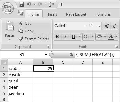
Figure 3-6. Cell B1 contains an array formula that returns the total number of characters contained in range A1:A5. Notice the brackets in the formula bar.
To demonstrate how an array formula can occupy more than one cell, create the worksheet shown in the figure and then try this:
Select the range B1:B5.
Type the following formula:
=LEN(A1:A5)
Press Ctrl+Shift+Enter.
The preceding steps enter a single array formula into five cells. Enter a SUM formula that adds the values in B1:B5, and you’ll see that the total number of characters in A1:A5 is 29.
Here’s the key point: It’s not necessary to actually display those five array elements. Rather, Excel can store the array in memory. Knowing this, you can type the following single array formula in any blank cell (Remember: Don’t type the curly brackets, and make sure that you enter it by pressing Ctrl+Shift+Enter):
{=SUM(LEN(A1:A5))}This formula essentially creates a five-element array (in memory) that consists of the length of each string in A1:A5. The SUM function uses this array as its argument, and the formula returns 29.
Figure 3-7 shows a worksheet set up to display a calendar for any month (change the month, and the calendar updates). Believe it or not, the calendar is created with a single array formula that occupies 42 cells.
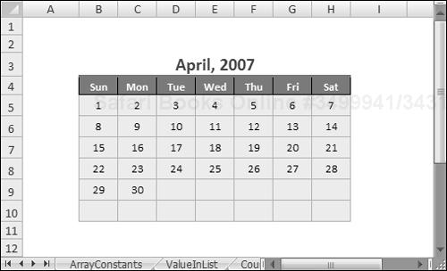
Figure 3-7. A single multicell array formula is all it takes to make a calendar for any month in any year.
The array formula, entered in the range B5:H10, is:
{=IF(MONTH(DATE(YEAR(B3),MONTH(B3),1))<>MONTH(DATE(YEAR(B3),
MONTH(B3),1)-(WEEKDAY(DATE(YEAR(B3),MONTH(B3),1))-1)
+{0;1;2;3;4;5}*7+{1,2,3,4,5,6,7}-1)," ",
DATE(YEAR(B3),MONTH(B3),1)-(WEEKDAY(DATE(YEAR(B3),
MONTH(B3),1))-1)+{0;1;2;3;4;5}*7+{1,2,3,4,5,6,7}-1)}The advantages of using array formulas rather than single-cell formulas include the following:
They can sometimes use less memory.
They can make your work much more efficient.
They can eliminate the need for intermediate formulas.
They can enable you to do things that would be difficult or impossible otherwise.
A few disadvantages of using array formulas are the following:
Using many complex array formulas can sometimes slow your spreadsheet recalculation time to a crawl.
They can make your worksheet more difficult for others to understand.
You must remember to enter an array formula with a special key sequence (by pressing Ctrl+Shift+Enter).
I spend quite a bit of time reading the Excel newsgroups on the Internet, and it seems that many of the questions deal with conditional counting or summing. In an attempt to answer most of these questions, I present a number of formula examples that deal with counting various things on a worksheet, based on single or multiple criteria. You can adapt these formulas to your own needs.
New
Excel 2007 includes two new counting and summing functions that aren’t available in previous versions (COUNTIFS and SUMIFS). Therefore, I present two versions of some formulas: an Excel 2007–only version and an array formula that works with all recent versions of Excel.
Figure 3-8 shows a simple worksheet to demonstrate the formulas that follow. The following range names are defined:
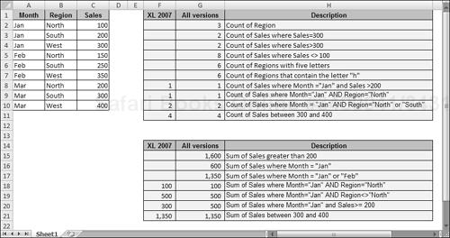
Month: A2:A10
Region: B2:B10
Sales: C2:C10
CD-ROM
This workbook (including the formula examples) is available on the companion CD-ROM. The file is named counting and summing examples.xlsx.
Table 3-3 contains formulas that demonstrate a variety of counting techniques.
Table 3-3. Counting Formula Examples
Formula | Description |
|---|---|
=COUNTIF(Region,”North”) | Counts the number of rows in which Region = “North” |
=COUNTIF(Sales,300) | Counts the number of rows in which Sales = 300 |
=COUNTIF(Sales,”>300”) | Counts the number of rows in which Sales > 300 |
=COUNTIF(Sales,”<>100”) | Counts the number of rows in which Sales <> 100 |
=COUNTIF(Region,”?????”) | Counts the number of rows in which Region contains five letters |
=COUNTIF(Region,”*h*”) | Counts the number of rows in which Region contains the letter H (not case-sensitive) |
=COUNTIFS(Month,”Jan”,Sales,”>200”) | Counts the number of rows in which Month = “Jan” and Sales > 200 (Excel 2007 only) |
{=SUM((Month=”Jan”)*(Sales>200))} | An array formula that counts the number of rows in which Month = “Jan” and Sales > 200 |
=COUNTIFS(Month,”Jan”,Region,”North”) | Counts the number of rows in which Month = “Jan” and Region = “North” (Excel 2007 only) |
{=SUM((Month=”Jan”)*(Region=”North”))} | An array formula that counts the number of rows in which Month = “Jan” and Region = “North” |
=COUNTIFS(Month,”Jan”,Region,”North”)+ COUNTIFS(Month,”Jan”,Region,”South”) | Counts the number of rows in which Month = “Jan” and Region = “North” or “South” (Excel 2007 only) |
{=SUM((Month=”Jan”)*((Region=”North”)+ (Region=”South”)))} | An array formula that counts the number of rows in which Month = “Jan” and Region = “North” or “South” |
=COUNTIFS(Sales,”>=300”,Sales,”<=400”) | Counts the number of rows in which Sales is between 300 and 400 (Excel 2007 only) |
{=SUM((Sales>=300)*(Sales<=400))} | An array formula that counts the number of rows in which Sales is between 300 and 400 |
Table 3-4 shows a number of formula examples that demonstrate a variety of summing techniques.
Table 3-4. Summing Formula Examples
Formula | Description |
|---|---|
=SUMIF(Sales,”>200”) | Sum of all Sales over 200 |
=SUMIF(Month,”Jan”,Sales) | Sum of Sales in which Month = “Jan” |
=SUMIF(Month,”Jan”,Sales)+ SUMIF(Month,”Feb”,Sales) | Sum of Sales in which Month =”Jan” or “Feb” |
=SUMIFS(Sales,Month,”Jan”,Region,”North”) | Sum of Sales in which Month=”Jan” and Region=”North” |
=SUMIFS(Sales,Month,”Jan”,Region,”North”) | Sum of Sales in which Month=”Jan” and Region=”North” (Excel 2007 only) |
{=SUM((Month=”Jan”)*(Region=”North”)*Sales)} | An array formula that returns the sum of Sales in which Month=”Jan” and Region=”North” |
=SUMIFS(Sales,Month,”Jan”,Region,”<>North”) | Sum of Sales in which Month=”Jan” and Region <> “North” (Excel 2007 only) |
{=SUM((Month=”Jan”)*(Region<>”North”)*Sales)} | An array formula that returns the sum of Sales in which Month=”Jan” and Region <> “North” |
=SUMIFS(Sales,Month,”Jan”,Sales,”>=200”) | Sum of Sales in which Month=”Jan” and Sales>=200 (Excel 2007 only) |
{=SUM((Month=”Jan”)*(Sales>=200)*(Sales))} | An array formula that returns the sum of Sales in which Month=”Jan” and Sales>=200 |
=SUMIFS(Sales,Sales,”>=300”,Sales,”<=400”) | Sum of Sales between 300 and 400 (Excel 2007 only) |
{=SUM((Sales>=300)*(Sales<=400)*(Sales))} | An array formula that returns the sum of Sales between 300 and 400 |
Excel uses a serial number system to store dates. The earliest date that Excel can understand is January 1, 1900. This date has a serial number of 1. January 2, 1900, has a serial number of 2, and so on.
Most of the time, you don’t have to be concerned with Excel’s serial number date system. You simply enter a date in a familiar date format, and Excel takes care of the details behind the scenes. For example, if you need to enter August 15, 2007, you can simply enter the date by typing August 15, 2007 (or use any of a number of different date formats). Excel interprets your entry and stores the value 39309, which is the serial number for that date.
Note
In this chapter, I assume the U.S. date system. If your computer uses a different date system, you’ll need to adjust accordingly. For example, you might need to enter 15 August 2007.
When working with times, you simply enter the time into a cell in a recognized format. Excel’s system for representing dates as individual values is extended to include decimals that represent portions or fractions of days. In other words, Excel perceives all time with the same system whether that time is a particular day, a certain hour, or a specific second. For example, the date serial number for August 15, 2007, is 39309. Noon (halfway through the day) is represented internally as 39309.5. Again, you normally don’t have to be concerned with these fractional serial numbers.
Because dates and times are stored as serial numbers, it stands to reason that you can add and subtract dates and times. For example, you can enter a formula to calculate the number of days between two dates. If cells A1 and A2 both contain dates, the following formula returns the number of intervening days:
=A2-A1
Tip
When performing calculations with time, things get a bit trickier. When you enter a time without an associated date, the date is assumed to be January 0, 1900 (date serial number 0). This is not a problem — unless your calculation produces a negative time value. When this happens, Excel displays an error (displayed as #########). The solution? Switch to the 1904 date system. Display the Excel Options dialog box, click the Advanced tab, and then enable the Use 1904 Date System check box. Be aware that switching to the 1904 date system can cause problems with dates already entered in your file or dates in workbooks that are linked to your file.
Tip
In some cases, you may need to use time values to represent duration, rather than a point in time. For example, you may need to sum the number of hours worked in a week. When you add time values, you can’t display more than 24 hours. For each 24-hour period, Excel simply adds another day to the total. The solution is to change the number formatting to use square brackets around the hour part of the format. The following number format, for example, displays more than 24 hours:
[hh]:mm
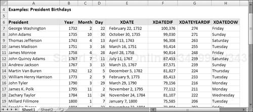
The world, of course, didn’t begin on January 1, 1900. People who work with historical information when using Excel often need to work with dates before January 1, 1900. Unfortunately, the only way to work with pre-1900 dates is to enter the date into a cell as text. For example, you can enter the following into a cell, and Excel won’t complain:
July 4, 1776
You can’t, however, perform any manipulation on dates that are actually text. For example, you can’t change its formatting, you can’t determine which day of the week this date occurred on, and you can’t calculate the date that occurs seven days later. (See Figure 3-9.)
Often, spreadsheets require intermediate formulas to produce a desired result. In other words, a formula may depend on other formulas, which in turn depend on other formulas. After you get all these formulas working correctly, it’s often possible to eliminate the intermediate formulas and use what I refer to as a single megaformula instead. The advantages? You use fewer cells (less clutter), the file size is smaller, and recalculation may even be a bit faster. The main disadvantage is that the formula may be impossible to decipher or modify.
Here’s an example: Imagine a worksheet that has a column with thousands of people’s names. And suppose that you’ve been asked to remove all the middle names and middle initials from the names — but not all the names have a middle name or initial. Editing the cells manually would take hours, and even Excel’s Data ![]() Data Tools
Data Tools ![]() Convert Text to Table command isn’t much help. So you opt for a formula-based solution. Although this is not a difficult task, it normally involves several intermediate formulas.
Convert Text to Table command isn’t much help. So you opt for a formula-based solution. Although this is not a difficult task, it normally involves several intermediate formulas.
Figure 3-10 shows the results of the more conventional solution, which requires six intermediate formulas shown in Table 3-5. The names are in column A; the end result goes in column H. Columns B through G hold the intermediate formulas.
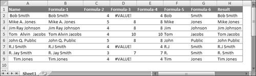
Table 3-5. Intermediate Formulas Written in Row 2 in Figure 3-9
Column | Intermediate Formula | What It Does |
|---|---|---|
B | =TRIM(A2) | Removes excess spaces. |
C | =FIND(“ “,B2,1) | Locates the first space. |
D | =FIND(“ “,B2,C2+1) | Locates the second space. Returns #VALUE! if there is no second space. |
E | =IF(ISERROR(D2),C2,D2) | Uses the first space if no second space exists. |
F | =LEFT(B2,C2) | Extracts the first name. |
G | =RIGHT(B2,LEN(B2)-E2) | Extracts the last name. |
H | =F2&G2 | Concatenates the two names. |
You can eliminate the six intermediate formulas by creating a megaformula. You do so by creating all the intermediate formulas and then going back into the final result formula and replacing each cell reference with a copy of the formula in the cell referred to (without the equal sign). Fortunately, you can use the Clipboard to copy and paste. Keep repeating this process until cell H2 contains nothing but references to cell A2. You end up with the following megaformula in one cell:
=LEFT(TRIM(A2),FIND
(" ",TRIM(A2),1))&RIGHT(TRIM(A2),LEN(TRIM(A2))-
IF(ISERROR(FIND(" ",TRIM(A2),FIND(" ",TRIM(A2),1)+1)),
FIND(" ",TRIM(A2),1),FIND(" ",TRIM(A2),FIND
(" ",TRIM(A2),1)+1)))
When you’re satisfied that the megaformula is working, you can delete the columns that hold the intermediate formulas because they are no longer used.
The megaformula performs exactly the same tasks as all the intermediate formulas — although it’s virtually impossible for anyone to figure out, even the author. If you decide to use megaformulas, make sure that the intermediate formulas are performing correctly before you start building a megaformula. Even better, keep a single copy of the intermediate formulas somewhere in case you discover an error or need to make a change.
Another way to approach this problem is to create a custom worksheet function in VBA. Then you could replace the megaformula with a simple formula, such as
=NOMIDDLE(A1)
In fact, I wrote such a function to compare it with intermediate formulas and megaformulas. The listing follows.
Function NOMIDDLE(n) As String
    Dim FirstName As String, LastName As String
    n = Application.WorksheetFunction.Trim(n)
    FirstName = Left(n, InStr(1, n, " "))
    LastName = Right(n, Len(n) - InStrRev(n, " "))
    NOMIDDLE = FirstName & LastName
End Function
CD-ROM
A workbook that contains the intermediate formulas, the megaformula, and the NOMIDDLE VBA function is available on the companion CD-ROM. The workbook is named megaformula.xlsm.
Because a megaformula is so complex, you may think that using one would slow down recalculation. Actually, that’s not the case. As a test, I created a worksheet that used a megaformula to process 150,000 names. Then I created another worksheet that used six intermediate formulas. The megaformula version calculated a bit faster, and produced a much smaller file.
The actual results will vary significantly, depending on system speed, amount of memory installed, and the actual formula.
The VBA function was much slower — I abandoned the timed test after 10 minutes. This is fairly typical of VBA functions; they are always slower than built-in Excel functions.