PivotTable field names come from the column headings used in the original source data. However, if you are using an external data source, the field names come from the names used in the data source's fields. If you do not like some or all of the field names in your PivotTable, you can rename them. Excel will remember the new names you specify and even preserve them when you refresh or rebuild the PivotTable. Note, however, that Excel does not change the corresponding headings in the source data.

Why rename a field? Usually because the original name is not suitable in some way. For example, many field names consist of multiple words that have been joined to avoid spaces, so you might have field names such as CustomerName and OrderDate. Renaming these fields to Customer Name and Order Date makes them easier to read. Similarly, you might have field names that are all uppercase letters and you might prefer to use title case, instead. Many PivotTable users prefer to change the name of the data field. Excel's default is "Sum of FieldName," where FieldName is the name of the field used in the summary calculation. A better name might use the form "FieldName Total" or something similar.

Rename a PivotTable Field

Note

This chapter uses the PivotTables.xls spreadsheet, available at www.wiley.com/go/pivottablesvb, or you can create your own sample database.

You can also double-click the field button or click the Field Settings button (

The PivotTable Field dialog box appears.

Note

Make sure that the new name you use does not conflict with an existing field name.

Extra

The field buttons you see in a PivotTable are not true command buttons, such as, for example, the OK and Cancel buttons in a dialog box. Instead, a PivotTable field button is really just a worksheet cell that has had special formatting applied. This means that when you click a field button, the button text appears inside Excel's formula bar. So an easier way to rename a PivotTable field is to click its button and then edit the button text that appears in the formula bar. You can also press F2 and edit the text directly in the cell. Note that when you use this method, Excel automatically updates the field name in the PivotTable Field List.

If you use this method to rename the page field, note that you will lose any text formatting that you have applied to the button text; see the task "Format a PivotTable Cell," later in this chapter. This appears to be a bug in Excel. To avoid this problem, use the PivotTable Field dialog box to rename the page field. Also, Excel does not update the PivotTable Field List when you rename a page field using the direct method. You need to click the Refresh Data button (

The names of the items that appear in the PivotTable's row or column area are the unique values that Excel has extracted from the source data fields you have added to each area. Therefore, because the items come from the data itself, you might think that their names would be unchangeable. That is not true, however. You can rename any field item and Excel will "remember" that the new name corresponds with the original item. Excel preserves your new names even after you refresh or rebuild the PivotTable.

As with field names, you will usually want to rename an item when its existing name is unsuitable. For example, the original name might not be very descriptive, it might be obscure, or it may come from a data source that uses all-uppercase or (more rarely) all-lowercase letters.

You should exercise a bit of caution when renaming items, however. If the people reading your report are familiar with the underlying data, they could become confused if you use names that differ significantly from the originals.

Remember, too, that renaming one or more items might cause the field to lose its current sort order. After you have finished renaming items in the field, you might need to resort the field, as described in the Chapter 4 task "Sort PivotTable Data with AutoSort."

Rename a PivotTable Item

Note

Make sure that the new name you use does not conflict with an existing item name in the same field. If you enter an existing name, Excel switches the position of the two items. In Chapter 4, see the task "Move Row and Column Items."

Apply It

The technique you learned in this task applies to items in the row and column areas. For obvious reasons, Excel does not allow you to edit any of the cells in the data area because they are all calculated values. That leaves only the page area. So how can you rename page field items if they do not reside in worksheet cells?

The solution is to pivot the page field you want to work with over to either the row or column area. Excel displays the field's items in cells, so you can then edit the items or items you want to rename. After you have finished renaming the items, pivot the field back to the page area. Excel preserves your new names in the page field drop-down list. Moreover, Excel sets up a correspondence between your new name and the item's original name in the source data. Therefore, when you select the renamed item in the page drop-down list, Excel filters the PivotTable results appropriately.

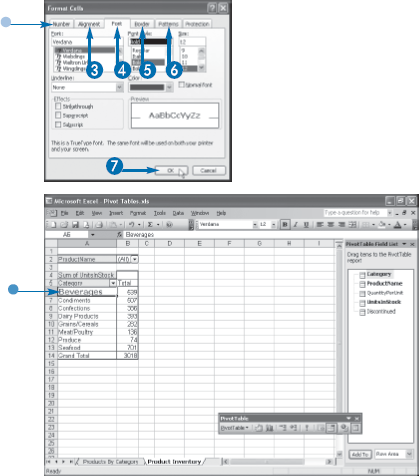
If you will be sharing your PivotTables with other people, via a network, e-mail, the Web, or a presentation, your report will have much more impact if it is nicely formatted and presented in a readable, eye-catching layout. You can use Excel's cell-formatting tools to apply a wide variety of formats to your PivotTable cells.

By default, Excel applies almost no formatting to PivotTable labels or data. The only exceptions are the borders that separate the PivotTable areas and the Grand Totals, and the special formatting that makes the field headings look like command buttons. However, you are free to modify the formatting for any cell in the PivotTable. For example, you can apply a numeric or date format, or create a custom format, as discussed in detail in the next three tasks of this chapter. You can also change the cell alignment to the left, center, or right, or you can wrap text within the cell. For the cell font, you can change the typeface, style, size, color, and more. You can also change the cell borders and apply background shading, either as a solid color or with a fill pattern.

By the way, the default format that the PivotTable Wizard applies to a new PivotTable is an AutoFormat called PivotTable Classic. Excel offers nearly two dozen PivotTable AutoFormats that enable you to apply a uniform format to an entire PivotTable. For the details, see the Chapter 6 task "Apply an AutoFormat." Excel also has a feature that preserves your formatting when you refresh your PivotTable; see the task "Preserve PivotTable Formatting," also in Chapter 6.

Format a PivotTable Cell

You can also select a range or a PivotTable area.

Note

To learn how to select PivotTable areas, see the Chapter 3 task "Select PivotTable Items."

You can also press Ctrl+1.

Excel displays the Format Cells dialog box.

Excel applies the formatting to the cell.

Extra

You can also format the selected cell or range using the following buttons on the Formatting toolbar:

Button	Description
	Applies a typeface.
	Sets the font size.
	Formats text as bold.
	Formats text as italics.
	Formats text as underlined.
	Left-aligns text.
	Centers text.
	Right-aligns text.
	Applies a border.
	Applies a background color.
	Applies a text color.

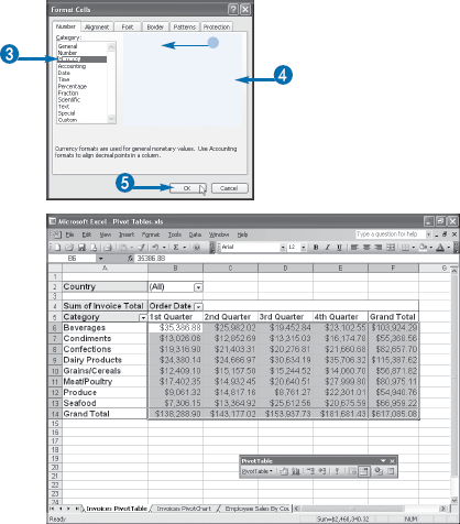
You can improve the readability of your PivotTable by applying the appropriate numeric formatting, such as displaying currency amounts with leading dollar signs and displaying large numbers with commas.

Excel offers six categories of numeric formats:

You can also create custom numeric formats. In Appendix A, see the section "Work with Custom Numeric and Date Formats."

Apply a Numeric Format to PivotTable Data

You can also press Ctrl+1.

To apply a numeric format to an entire field, double-click the field button and then click Number.

Excel displays the Format Cells dialog box.

Excel applies the numeric formatting to the cell or range.

Extra

You can also set the numeric format of the selected cell or range by applying a style. Click Format→Style and then click the numeric style you want: Comma, Currency, or Percent. You can also set the numeric format using the following buttons on the Formatting toolbar:

Button	Description
	Applies the Currency style.
	Applies the Percent style.
	Applies the Comma style.
	Increases the number of decimal places.
	Decreases the number of decimal places.

There are also a few shortcut keys you can use to set the numeric format:

Press	To Apply the Format
Ctrl+~	General
Ctrl+!	Number (2 decimal places; using the thousands separator)
Ctrl+$	Currency (2 decimal places; using the dollar sign; negative numbers surrounded by parentheses)
Ctrl+%	Percentage (0 decimal places)
Ctrl+^	Scientific (2 decimal places)

If you include dates or times in your PivotTables, you need to make sure that they are presented in a readable, unambiguous format. For example, most people would interpret the date 8/5/06 as August 5, 2006. However, in some countries this date would mean May 8, 2006. Similarly, if you use the time 2:45, do you mean AM or PM? To avoid these kinds of problems, you can apply Excel's built-in date and time formats to a PivotTable cell or range.

The Date format specifies how Excel displays the date components — the day, month, and year — as well as which symbol to use to separate the components. For the month component of the date, Excel can display any of the following: the number (where January is 1, February is 2, and so on) with or without a leading 0; the first letter of the month name (for example, M for March); the abbreviated month name (for example, Mar for March); or the full month name. For the year component, Excel can display either the final two digits (for example, 06 for 2006) or all four digits. You can also choose either a slash (/) or a hyphen (-) to separate the date components. Depending on the location you choose, such as the United States or Canada, you may also be able to include the day of the week or use a period (.) as the date separator.

The Time format specifies which time components — hours, minutes, and seconds — Excel displays. You can also choose whether Excel uses regular time (for example, 1:30:55 PM) or military time (for example, 13:30:55). When you select a regular time format, Excel always includes either AM or PM; when you choose a military time format, Excel does not include AM or PM.

You can also create custom date formats. In Appendix A, see the section "Work with Custom Numeric and Date Formats."

Apply a Date Format to PivotTable Data

You can also press Ctrl+1.

To apply a date or time format to an entire field, double-click the field button and then click Number.

Excel displays the Format Cells dialog box.

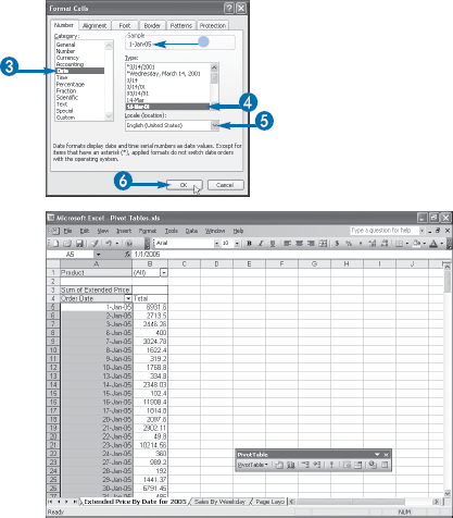
If you are formatting times, click Time, instead.

Excel applies the date or time formatting to the cell or range.

Extra

There are a few shortcut keys you can use to set the date or time format as well as to add the current date or time:

Press	To
Ctrl-#	Apply the date format 14-Mar-01
Ctrl-@	Apply the time format 1:30 PM
Ctrl-;	Enter the current date using the format 3/14/2001
Ctrl-:	Enter the current time using the format 1:30 PM

In the Number tab of the Format Cells dialog box, if you click the Date format and choose English (United States) in the Locale list, Excel shows two date formats at the top of the Type list:

*3/14/2001
*Wednesday, March 14, 2001

The asterisks tell you that the order of the date components may change if someone opening the worksheet is using a different locale. For example, if you select the *3/14/2001 format, a user in the United Kingdom will likely see the date as 14/3/2001. If you want to make sure that other users always see the dates as you format them, choose a format that does not have a leading asterisk.

Formatting numbers with thousands separators, decimals, or currency symbols is useful because a PivotTable is, in the end, a report, and reports should always look their best. However, the main purpose of a PivotTable is to perform data analysis, and regular numeric formatting achieves that goal only insofar as it helps you and others read and understand the report. However, if you want to extend the analytic capabilities of your PivotTables, you need to turn to a more advanced technique called conditional formatting.

The idea behind conditional formatting is that you want particular values in your PivotTable results to stand out from the others. For example, if your PivotTable tracks product inventory, you might want to be alerted when the inventory of any item falls below some critical value. Similarly, you might want to track the total amount sold by your salespeople and be alerted when an employee's results exceed some value so that, say, a bonus can be awarded.

Conditional formatting enables you to achieve these and similar results. With a conditional format applied to some or all of the PivotTable's data area, Excel examines the numbers and then applies formatting — a font, border, and pattern that you specify — to any cells that match your criteria. By applying, say, a bold font, thick cell border, and a background color to results that satisfy your criteria, you can find those important results with a quick glance at your PivotTable.

Note, however, that conditional formatting only works with PivotTables that have a static layout. The conditional formatting is a property of the cells to which you apply it, not of the PivotTable. So, for example, if you pivot the column field into the row area, your conditional formatting does not travel with the field.

Apply a Conditional Format to PivotTable Data

The Conditional Formatting dialog box appears.

Excel displays the Format Cells dialog box.

Excel returns you to the Conditional Formatting dialog box.

Excel applies the conditional formatting to the range.

Apply It

There may be times when you want to apply multiple conditional formats to your PivotTable results. For example, in an inventory report, you might want to apply one format when a product's inventory level falls below some threshold, and a second format when the inventory is zero. Similarly, for employee sales, you can establish multiple sales thresholds and assign a conditional format for each one. For these and similar situations, Excel enables you to define up to three different conditional formats — named Condition 1, Condition 2, and Condition 3.

Follow Steps 1 and 2 to display the Conditional Formatting dialog box. Enter your criteria and format options for Condition 1, and then click Add. Excel expands the dialog box to show the controls for Condition 2. You specify the criteria and formatting for Condition 2 in the same way as you did for Condition 1. If you need a third condition, click Add again to expand the dialog box to show the Condition 3 controls.

If you decide later that you no longer require one or more of these conditions, display the Conditional Formatting dialog box, click Delete, select each condition you want to remove (

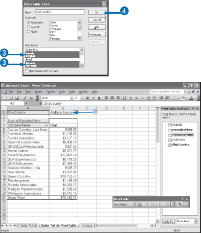
A PivotTable report is meant to be a succinct summary of a large quantity of data. One way that Excel increases the succinctness of a PivotTable is to exclude from the report any items that have no data. This is usually the behavior that you want, but it can cause some problems with certain kinds of reports.

One of the problems that comes up when some items have no data concerns filtering the report using a page field. For example, suppose there are two items in the page field, and that a particular row item has data for the first page field item, but it has no data for the second page field item. When you switch pages, your PivotTable layout will change because Excel removes the row field item from the report when you filter on the second page field.

Another problem occurs when you group the PivotTable results. If no results fall within a particular grouping, Excel does not display the grouping.

In both cases, the exclusion of a field item or grouping can be confusing and, in any case, you may be interested in seeing items or groupings that have no data.

You can work around these problems by forcing Excel to always show field items that have no data, as described in this task.

Show Items with No Data

You can also double-click the field button or click the Field Settings button (

The PivotTable Field dialog box appears.

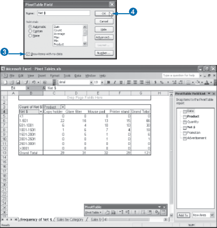
Excel displays the PivotTable report with items that have no data.

Apply It

One PivotTable problem that comes up more often than you might think is when you end up with "phantom" field items, or items that no longer exist in the source data. This occurs when an item appears originally in the source data, shows up in a PivotTable report, and is then subsequently renamed in or deleted from the source data. When you refresh the PivotTable, the item disappears. However, if you activate "Show items with no data" (

The only way to solve this problem is to use VBA to delete the PivotTable item. Here is a VBA macro that deletes the PivotTable item in the active worksheet cell:

Example:

Sub DeletePivotTableItem()
    Dim nResult As Integer
    '
    ' Work with the PivotItem object in the active cell
    With ActiveCell.PivotItem
        '
        ' Confirm the deletion
        nResult = MsgBox("Are you sure you want " & _
                  "to delete the """ & _
                  .Value & """ item?", vbYesNo)
        '
        ' If Yes, delete the PivotItem object
        If nResult = vbYes Then .Delete
    End With
End Sub

You can configure your PivotTable to hide multiple page field items and thus display a subset of the pages in your PivotTable results.

In a default PivotTable that includes a page field, Excel displays the results for all items in the page field. In Chapter 4, you learned how to display the results for a single page; see the task "Display a Different Page." However, there may be times when you need to display the results for more than one page, although not all the pages. For example, you may know that the results from one or more pages are incomplete or inaccurate, and so should not be included in the report. Alternatively, your data analysis may require that you view the PivotTable results for only a subset of pages.

For these and similar situations, Excel enables you to customize the page field to exclude one or more items. Excel then redisplays the PivotTable without showing those items or including their results in the PivotTable totals. However, it is possible to include the results of hidden page fields in your PivotTable totals. In Chapter 7, see the task "Include Hidden Pages in PivotTable Results."

Exclude Items from a Page Field

You can also double-click the field button or click the Field Settings button (

The PivotTable Field dialog box appears.

Excel redisplays the PivotTable without the page field items you selected.

Apply It

Excel does not offer an easy way to add hidden page items back into the page field list. You need to open the PivotTable Field dialog box again and click each item that you hid earlier. To make this chore easier, you can include all page field items via VBA by setting the Visible property of each page field PivotItem object to True, as shown in the following macro:

Example:

Sub ShowAllPageFieldItems()
    Dim objPT As PivotTable
    Dim objPageField As PivotField
    Dim objPageItem As PivotItem
    '
    ' Work with the first PivotTable on the active worksheet
    Set objPT = ActiveSheet.PivotTables(1)
    '
    ' Work with the first page field
    Set objPageField = objPT.PageFields(1)
    '
    ' Run through all the page field items
    For Each objPageItem In objPageField.PivotItems
        '
        ' Display the item
        objPageItem.Visible = True
    Next 'objPageItem
End Sub