In the Chapter 5 task "Format a PivotTable Cell," you learned how to apply formatting options such as alignments and fonts to portions of a PivotTable. This works well, particularly if you have custom formatting needs. For example, you may have in-house style guidelines that you need to follow. Unfortunately, applying formatting can be time-consuming, particularly if you are applying a number of different formatting options. And the total formatting time can become onerous if you need to apply different formatting options to different parts of the PivotTable. You can greatly reduce the time you spend formatting your PivotTables if you instead apply an AutoFormat.

An AutoFormat is a collection of formatting options — alignments, fonts, borders, and patterns — that Excel defines for different areas of a PivotTable. For example, an AutoFormat might use bold, black text on a yellow background for items, italics for grand totals and subtotals, and alternating white and gray backgrounds for columns. Defining all these formats by hand might take a half an hour to an hour. But with the AutoFormat feature, you choose the one you want to use for the PivotTable as a whole, and Excel applies the individual formatting options automatically.

Excel defines 22 AutoFormats, including PivotTable Classic, the default formatting applied to reports you create using the PivotTable Wizard, and None, which removes all formatting from the PivotTable. The other AutoFormats are named Report 1 through Report 10 and Table 1 through Table 8. Bear in mind that some AutoFormats change the layout of the PivotTable. For example, any of the "Report" AutoFormats will move the column field to the row area as the outer field. Similarly, any of the "Table" AutoFormats will move the row area's outer field to the column area.

Apply an AutoFormat

Note

This chapter uses the PivotTables.xls spreadsheet, available at www.wiley.com/go/pivottablesvb, or you can create your own sample database.

The AutoFormat dialog box appears.

Excel applies the AutoFormat.

Apply It

You can use VBA to set your favorite AutoFormat. Each PivotTable object has a Format property that you can set to a constant value that corresponds to the AutoFormat you want to apply. The constants are xlReport1 through xlReport10, xlTable1 through xlTable8, xlPTClassic, and xlPTNone. Here is a macro that applies the Report 1 AutoFormat:

Example:

Sub ApplyAutoFormat()
    '
    ' Apply Report 1 AutoFormat to first PivotTable on active worksheet
    ActiveSheet.PivotTables(1).Format xlReport1
End Sub

Here is another macro that applies the PivotTable Classic AutoFormat:

Example:

Sub ApplyClassicAutoFormat()
    '
    ' Apply Classic AutoFormat to first PivotTable on active worksheet
    ActiveSheet.PivotTables(1).Format xlPTClassic
End Sub

You may find that Excel does not preserve your custom formatting when you refresh or rebuild the PivotTable. For example, if you applied a bold font to some labels, that text may revert to regular text after a refresh. Excel has a feature called Preserve Formatting that enables you to preserve such formatting during a refresh, so you can retain your custom formatting by activating this feature.

The Preserve Formatting feature is always activated in default PivotTables. However, it is possible that another user can deactivate this feature. For example, you may be working with a PivotTable created by another person and he or she deactivated the Preserve Formatting feature.

Note, however, that when you refresh or rebuild a PivotTable, Excel reapplies the report's current AutoFormat. If you have not specified an AutoFormat, Excel reapplies the default PivotTable Classic AutoFormat; if you have specified an AutoFormat — as described in the previous task, "Apply an AutoFormat" — Excel reapplies that AutoFormat.

Also, Excel always preserves your numeric formats and date formats. In Chapter 5, see the tasks "Apply a Numeric Format to PivotTable Data" and "Apply a Date Format to PivotTable Data."

Preserve PivotTable Formatting

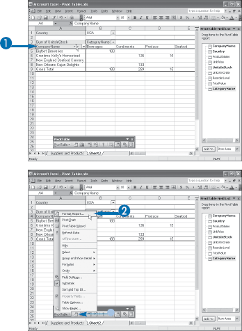
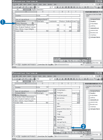
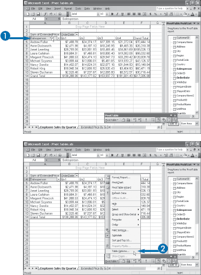
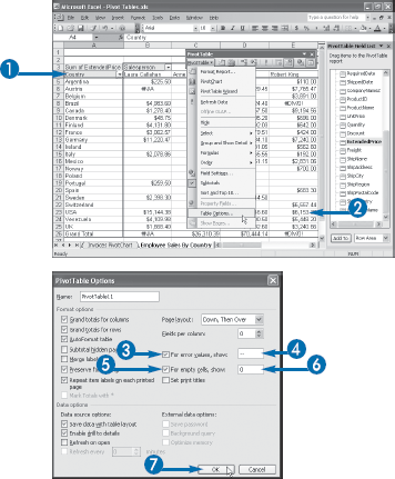
You can also right-click any PivotTable cell and then click Table Options.

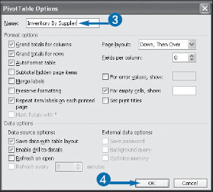
The PivotTable Options dialog box appears.

Note

Deselecting this check box prevents Excel from automatically formatting things such as column widths when you pivot fields.

Excel preserves your custom formatting each time you refresh the PivotTable.

Apply It

In VBA, you use the PivotTable object's PreserveFormatting property to turn the Preserve Formatting feature on (True) or off (False). Here is a VBA procedure that toggles the value of this property between True and False:

Example:

Sub TogglePreserveFormatting()
    Dim objPT As PivotTable
    '
    ' Work with the first PivotTable on the active worksheet
    Set objPT = ActiveSheet.PivotTables(1)
    With objPT
        '
        ' Toggle the PreserveFormatting property
        .PreserveFormatting = Not .PreserveFormatting
        '
        ' Display the new setting
        MsgBox "The Preserve Formatting feature is now " & _
            IIf(.PreserveFormatting, "activated.", "deactivated.")
    End With
End Sub

When you create the first PivotTable in a workbook, Excel gives it the default name PivotTable1. Subsequent PivotTables are named sequentially: PivotTable2, PivotTable3, and so on. If your workbook contains a number of PivotTables, you can make them easier to distinguish by giving each one a unique and descriptive name.

Why do you need to provide your PivotTables with descriptive names? The main benefit occurs after you have built a PivotTable based on a particular data source. If you then attempt to build a second PivotTable based on the same data source, Excel displays a dialog box that tells you the new report will use less memory if you base it on the first PivotTable instead of the data source itself. Recall that each PivotTable maintains a pivot cache, which is a snapshot of the data source, so your new PivotTable can share this pivot cache and your workbook will be much smaller.

However, if you elect to base your new PivotTable on an existing report, Excel asks you which report you want to use and it displays a list of the PivotTable names in the open workbooks. Excel always selects the report that it thinks you should use, but it is difficult to tell if that is the correct one if all the PivotTables use generic names such as PivotTable1 and PivotTable2. If, instead, you provide your PivotTables with descriptive names, you can easily tell them apart and select the correct report upon which to base your new PivotTable.

Rename the PivotTable

You can also right-click any PivotTable cell and then click Table Options.

The PivotTable Options dialog box appears.

Note

The maximum length for a PivotTable name is 255 characters.

Excel renames the PivotTable.

Apply It

If you use VBA to manipulate PivotTables, using unique names to reference PivotTable objects can make your code easier to read. For example, to reference a PivotTable named "Budget Summary" that exists in a worksheet named "Sheet1," you use the following statement:

Worksheets("Sheet1).PivotTables("Budget Summary")

What happens, however, if your workbook contains a large number of PivotTables? Rather than renaming each one by hand, you could use the following macro to rename each one automatically using the worksheet name:

Sub RenameAllPivotTables()
    Dim objWS As Worksheet
    Dim objPT As PivotTable
    Dim i As Integer
    '
    ' Run through all the worksheets
    For Each objWS In ThisWorkbook.Worksheets
        i = 1
        '
        ' Run through all the PivotTables
        For Each objPT In objWS.PivotTables
            '
            ' Rename it to the sheet name plus the value of i
            objPT.Name = objWS.Name & " " & i
            i = i + 1
        Next 'objPT
    Next 'objWS
End Sub

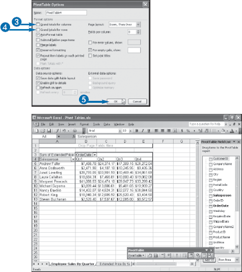
You can configure your PivotTable to not display the Grand Total row or the Grand Total column (or both). This is useful if you want to save space in the PivotTable or if the grand totals are not relevant in your data analysis.

A default PivotTable that has at least one row field contains an extra row at the bottom of the table. This row is labeled Grand Total and it includes the total of the values associated with the row field items. However, the value in the Grand Total row may not actually be a sum. For example, if the summary calculation is Average, then the Grand Total row includes the average of the values associated with the row field items. To learn how to use a different summary calculation, see the Chapter 7 task "Change the PivotTable Summary Calculation."

Similarly, a PivotTable that has at least one column field contains an extra column at the far right of the table. This column is also labeled "Grand Total" and it includes the total of the values associated with the column field items. If the PivotTable contains both a row and a column field, the Grand Total row also has the sums for each column item, and the Grand Total column also has the sums for each row item.

Besides taking up space in the PivotTable, these grand totals are often not necessary for data analysis. For example, suppose you want to examine quarterly sales for your salespeople to see which amounts were over a certain value for bonus purposes. Because your only concern is the individual summary values for each employee, the grand totals are useless. In such a case, you can tell Excel not to display the grand totals.

Turn Off Grand Totals

You can also right-click any PivotTable cell and then click Table Options.

The PivotTable Options dialog box appears.

Excel displays the PivotTable without the grand totals.

Apply It

You can work with grand totals via VBA using the PivotTable object's ColumnGrand and RowGrand properties, which are Boolean values that hide (False) and display (True) the grand totals. The following macro toggles these properties on and off:

Example:

Sub ToggleGrandTotals()
    Dim objPT As PivotTable
    '
    ' Work with the first PivotTable on the active worksheet
    Set objPT = ActiveSheet.PivotTables(1)
    With objPT
        '
        ' Toggle the ColumnGrand and RowGrand properties
        .ColumnGrand = Not .ColumnGrand
        .RowGrand = Not .RowGrand
        '
        ' Display the new setting
        MsgBox "The grand totals are now " & _
            IIf(.ColumnGrand, "displayed.", "hidden.")
    End With
End Sub

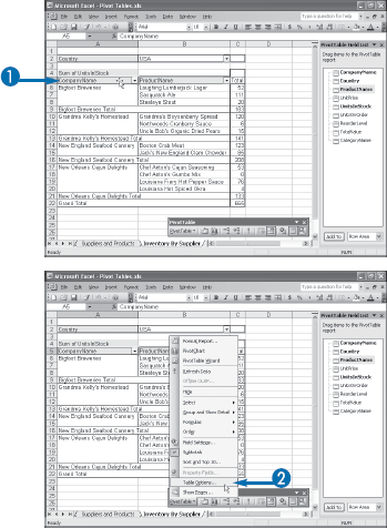
If you have a PivotTable with multiple fields either in the row area or the column area, you can make the outer field easier to read by merging the cells associated with each of the field's item labels.

When you configure a PivotTable with two fields in the row area, Excel displays the outer field on the left and the inner field on the right. For each item in the outer field, Excel displays the item label in the left column, and then the associated inner field items in the right column. If the inner field has two or more associated items, then there will be one or more blank cells below the outer field item. This makes the PivotTable report less attractive and harder to read because the outer field items appear just below the subtotals.

A similar problem occurs when you have multiple fields in the column area. In this case, you can end up with one or more blank cells to the right of each outer field item.

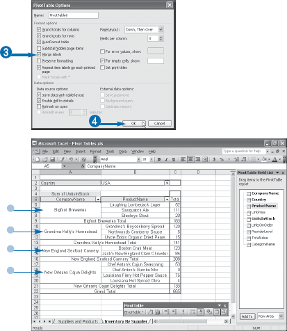
To fix these problems, you can activate a PivotTable option that tells Excel to merge the cells associated with each outer field item. Excel then displays the item label in the middle of these merged cells, which makes the PivotTable report more attractive and easier to read.

Merge Item Labels

You can also right-click any PivotTable cell and then click Table Options.

The PivotTable Options dialog box appears.

Excel merges the cells associated with each item in the outer row and outer column fields.

Apply It

In VBA you use the PivotTable object's MergeLabels property to turn the Merge Labels feature on (True) or off (False). Here is a VBA procedure that toggles the value of this property between True and False:

Example:

Sub ToggleMergeLabels()
    Dim objPT As PivotTable
    '
    ' Work with the first PivotTable on the active worksheet
    Set objPT = ActiveSheet.PivotTables(1)
    With objPT
        '
        ' Toggle the MergeLabels property
        .MergeLabels = Not .MergeLabels
        '
        ' Display the new setting
        MsgBox "The Merge Labels feature is now " & _
            IIf(.MergeLabels, "activated.", "deactivated.")
    End With
End Sub

You can improve the look of a PivotTable report by specifying alternative text to appear in place of error values and blank cells.

Excel has seven different error values: #DIV/0!, #N/A, #NAME?, #NULL!, #NUM!, #REF!, and #VALUE!. These errors are almost always the result of improperly constructed formulas, and because a basic PivotTable has no formulas, you rarely see error values in PivotTable results. There are two exceptions, however. First, if the source data field you are using for the PivotTable summary calculation contains an error value, then Excel reproduces that error value within the PivotTable results. Second, you can add a custom calculated field to the PivotTable, and that field's values will be based on a formula. For the details about calculated fields, see Chapter 8. If that formula generates an error, Excel displays the corresponding error value in the PivotTable results. For example, if your formula divides by 0, the #DIV/0! error appears. Seeing these errors is usually a good thing because it alerts you to problems in the data or the report. However, if the error is caused by something temporary, then you may prefer to hide any errors by displaying a blank or some other text, instead.

A related PivotTable concern is what to do with data area cells where the calculation results in a 0 value. By default, Excel displays nothing in the cell. This can make the report slightly easier to read, but it may also cause confusion for readers of the report. In an inventory PivotTable, for example, does an empty cell mean that the product has no stock or that it was not counted? To avoid this problem, you can specify that Excel display the number 0 or some other text instead of an empty cell.

Specify Characters for Errors and Empty Cells

You can also right-click any PivotTable cell and then click Table Options.

The PivotTable Options dialog box appears.

Apply It

In VBA you use the PivotTable object's ErrorString property to set the text to replace error values, and you use the DisplayErrorString property to turn this feature on and off. Also, you use the PivotTable object's NullString property to set the text to use in empty cells, and you use the DisplayNullString property to turn this feature on and off. Here is an example macro that uses these properties:

Sub SetTextForErrorsAndEmptyCells()
    Dim objPT As PivotTable
    '
    ' Work with the first PivotTable
    Set objPT = ActiveSheet.PivotTables(1)
    With objPT
        '
        ' Set ErrorString and activate it
        .ErrorString = "@@hy@@hy"
        .DisplayErrorString = True
        '
        ' Set NullString and activate it
        .NullString = "0"
        .DisplayNullString = True
        '
        ' Display the new settings
        MsgBox "The ErrorString text is" & _
         "now """ & .ErrorString & """" & _
         vbCrLf & _
         "The NullString text is " & _
         "now """ & .NullString & """"
    End With
End Sub

If you have a PivotTable that you will share with other people, but you do not want those people to make any changes to the report, you can activate protection for the worksheet that contains the PivotTable. This prevents unauthorized users from changing the PivotTable results.

If you have put a lot of work into the layout and formatting of a PivotTable, you most likely want to avoid having any of your work undone if you allow other people to open the PivotTable workbook. The easiest way to do this is to enable Excel's worksheet protection feature. When this feature is activated for a worksheet that contains a PivotTable, no user can modify any cells in the PivotTable. If needed, you can also apply a password to the protection, so that only authorized users can make changes to the worksheet.

Excel's default protection options affect PivotTables in two ways:

Protect a PivotTable

The Protect Sheet dialog box appears.

Note

Protecting the worksheet with a password is optional. However, without a password, it is very easy for a user to unprotect the worksheet.

If you specified a password in Step 4, Excel asks you to confirm the password.

Excel protects the worksheet.

Extra

When you protect a worksheet, you may be willing to let users modify certain cells on the worksheet. In a PivotTable, for example, you may want to allow users to rename the PivotTable fields or items. You can set this up by unlocking those cells before you activate worksheet protection. Begin by selecting the cells that you will allow users to edit. Then click Format→Cells to display the Format Cells dialog box. Click the Protection tab, deselect Locked (

When you want to make changes to a PivotTable on a protected worksheet, you must first unprotect the worksheet. Display the protected worksheet and then click Tools→Protection→Unprotect Sheet. If you protected the worksheet with a password, Excel displays a dialog box that asks you for the password. Type the password and then click OK. Excel unprotects the worksheet.