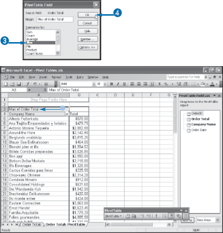
If you add a numeric field to the data area, Excel uses Sum as the default summary calculation. If, instead, you use a text field in the data area, Excel uses Count as the default summary calculation. If your data analysis requires a different calculation, you can configure the data field to use any one of Excel's 11 built-in summary calculations:
Sum — Adds the values in a numeric field.
Count — Displays the total number of cells in the source field.
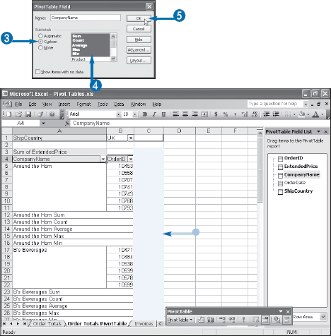
Average — Calculates the mean value in a numeric field.
Max — Displays the largest value in a numeric field.
Min — Displays the smallest value in a numeric field.
Product — Multiplies the values in a numeric field.
Count Nums — Displays the total number of numeric values in the source field.
StdDev — Calculates the standard deviation of a population sample, which tells you how much the values in the source field vary with respect to the average.
StdDevp — Calculates the standard deviation when the values in the data field represent the entire population.
Var — Calculates the variance of a population sample; the variance is the square of the standard deviation.
Varp — Calculates the variance when the values in the data field represent the entire population.
Note
This chapter uses the PivotTables.xls spreadsheet, available at www.wiley.com/go/pivottablesvb, or you can create your own sample database.
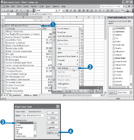
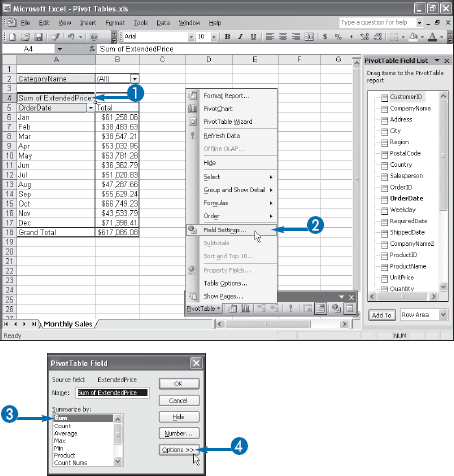
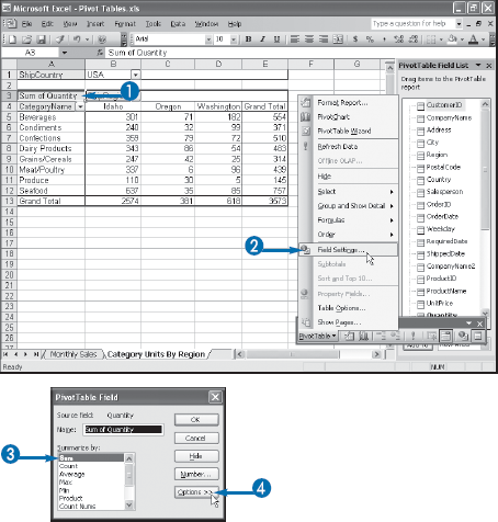
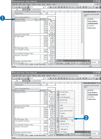
You can also double-click the data field button or click the Field Settings button (
The PivotTable Field dialog box appears.
Excel recalculates the PivotTable results.
Extra
When you build your PivotTable, you may find that the results do not look correct. For example, the number may appear to be far too small. In that case, check the summary calculation that Excel has applied to the field to see if it is using Count instead of Sum. If the data field includes one or more text cells or one or more blank cells, Excel defaults to the Count summary function instead of Sum. If your field is supposed to be numeric, check the data to see if there are any text values or blank cells.
When you add a second field to the row or column area — see the Chapter 3 task "Add Multiple Fields to the Row or Column Area" — Excel displays a subtotal for each item in the outer field. By default, that subtotal shows the sum of the data results for each outer field item. However, the same 11 summary calculations — from Sum to Varp — are also available for subtotals.
To change the subtotal summary calculation for a row or column field, click the outer field button and then click PivotTable→Field Settings to display the PivotTable Field dialog box. Select Custom (
You can use Excel's difference calculations to compare the items in a numeric field and return the difference between them.
The built-in summary calculations — Sum, Count, Average, and so on — apply over an entire field. However, a major part of data analysis involves comparing one item with another. If you are analyzing sales to customers, for example, it is useful to know how much you sold this year, but it is even more useful to compare this year's sales with last year's. Are the sales up or down? By how much? Are the sales up or down with all customers or only some? These are fundamental questions that help managers run departments, divisions, and companies.
Excel offers two difference calculations that can help you perform this kind of analysis:
Before you set up a difference calculation, you need to decide which field in your PivotTable you will use as the comparison field — the base field — and which item within that field you will use as the basis for all the comparisons — the base item. For example, if you are comparing the sales in 2005 to the sales in 2004, the date field is the base field and 2004 is the base item.
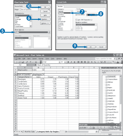
You can also double-click the data field button or click the Field Settings button (
The PivotTable Field dialog box appears.
Excel expands the dialog box.
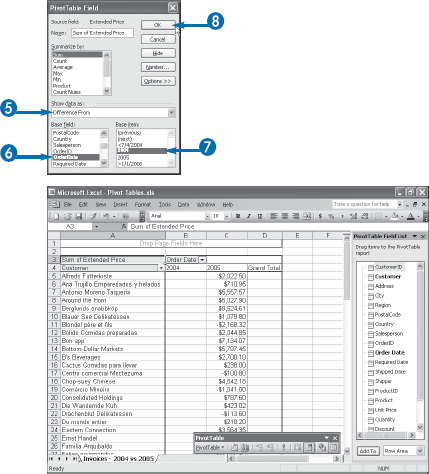
If you want to see the difference in percentage terms, click % Difference From, instead.
Excel recalculates the PivotTable results.
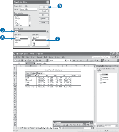
You can use Excel's percentage calculations to view data items as a percentage of some other item or as a percentage of the total in the current row, column, or PivotTable.
Percentage calculations are useful data analysis tools because they enable you to make apples-to-apples comparisons between values. For example, suppose your PivotTable shows that sales to a particular customer increased by $25,000 this year. Is that good or bad? The answers depend on the total sales. If the sales last year were $25,000, then the increase is good; if the previous year's sales were $250,000, then the increase is not so good. To make this clear, you need to find out the percentage increase: a $25,000 increase on $25,000 sales is a rise of 100%, while the same increase on sales of $250,000 is only 10%.
Excel offers four percentage calculations that can help you perform this kind of analysis:
% Of — Returns the percentage of each value with respect to a selected base item.
% of Row — Returns the percentage that each value in a row represents of the total value of the row.
% of Column — Returns the percentage that each value in a column represents of the total value of the column.
% of Total — Returns the percentage that each value represents of the PivotTable grand total.
As with the difference calculations you learned about in the previous task, "Create a Difference Summary Calculation," if you use the % Of calculation, you must also choose a base field and a base item upon which Excel will calculate the percentages.

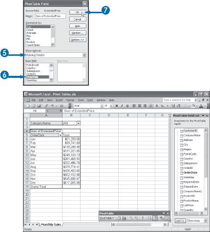
You can use Excel's Running Total calculation to view the PivotTable results as values that accumulate as they run through the items in a row or column field.
A running total is the cumulative sum of the values that appear in a given set of data. Most running totals accumulate over a period of time. For example, suppose you have 12 months of sales figures. In a running total calculation, the first value is the first month of sales, the second value is the sum of the first and second months, the third value is the sum of the first three months, and so on.
You use a running total in data analysis when you need to see a snapshot of the overall data at various points. For example, suppose you have a sales budget for each month. As the fiscal year progresses, comparing the running total of the budget figures with the running total of the actual sales tells you how your department or company is doing with respect to the budget. If sales are consistently below budget, you might consider lowering prices, offering customers extra discounts, or increasing your product advertising.
Excel offers a Running Total summary calculation that you can apply to your PivotTable results. Note, too, that the Running Total applies not just to the Sum calculation, but also to related calculations such as Count and Average. Before you configure your PivotTable to use a Running Total summary calculation, you must decide the field on which to base the accumulation, or the base field. This will most often be a date field, but you can also create running totals based on other fields, such as customer, division, product, and so on.
You can use Excel's Index calculation to determine the relative importance of the results in your PivotTable.
One of the most crucial aspects of data analysis is determining the relative importance of the results of your calculations. This is particularly true in a PivotTable, where the results summarize a large amount of data, but on the surface, provide no clue as to the relative importance of the various data area values.
For example, suppose your PivotTable shows the units sold for various product categories, broken down by state. Suppose further that in Oregon you sold 30 units of Produce and 35 units of Seafood. Does this mean that Seafood sales are relatively more important in the Oregon market than Produce sales? Not necessarily. To determine relative importance, you must take the larger picture into account. For example, you must look at the total units sold of both Produce and Seafood across all states. Suppose the Produce total is 145 units and the Seafood total is 757 units. You can see that the 30 units of Produce sold in Oregon represents a much higher portion of total Produce sales than does Oregon's 35 units of Seafood. A proper analysis would also take into account the total units sold in Oregon and the total units sold overall (the Grand Total).
This sounds complex, but Excel's Index calculation handles everything easily. The Index calculation determines the weighted average of each cell in the PivotTable results. Here is the formula Excel uses:
(Cell Value) * (Grand Total) / (Row Total) * (Column Total)
In the resulting numbers, the higher the value, the more important the cell is in the overall results.
You can also double-click the data field button or click the Field Settings button (
The PivotTable Field dialog box appears.
Excel expands the dialog box.
The Format Cells dialog box appears.
You are returned to the PivotTable Field dialog box.
Excel recalculates the PivotTable results.
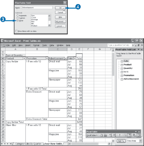
You can make a multiple-field row or column area easier to read by turning off the display of subtotals.
When you add a second field to the row or column area, as described in the Chapter 3 task "Add Multiple Fields to the Row or Column Area," Excel automatically displays subtotals for the items in the outer field. This is a useful component of data analysis because it shows you not only how the data breaks down according to the items in the second (inner) field, but also the total of those items for each item in the first (outer) field.
If you add a third field to the row or column area, Excel displays two sets of subtotals: one for the second (middle) field and one for the first (outer) field. And for every extra field you add to the row or column area, Excel adds another set of subtotals.
A PivotTable displaying two or more sets of subtotals in one area can be quite confusing to read. You can reduce the complexity of the PivotTable layout by turning off the subtotals for one or more of the fields.
You can extend your data analysis by reconfiguring your PivotTable results to show more than one type of subtotal for a given field.
When you add a second field to the row or column area, as described in the Chapter 3 task "Add Multiple Fields to the Row or Column Area," Excel displays a subtotal for each item in the outer field, and that subtotal uses the Sum calculation. If you prefer to see the Average for each item or the Count, you can change the field's summary calculation; see the task "Change the PivotTable Summary Calculation," earlier in this chapter.
However, it is a common data analysis task to view items from several different points of view. That is, you may want to study the results by seeing not just a single summary calculation, but several: Sum, Average, Count, Max, Min, and so on. Unfortunately, it is not convenient to switch from one summary calculation to another. To avoid this problem, Excel enables you to view multiple subtotals for each field, where each subtotal uses a different summary calculation. You can use as many of Excel's 11 built-in summary calculations as you need. Note, however, that it does not make sense to use StdDev and StDevp at the same time, because the former is for sample data and the later is for population data. The same is true for the Var and Varp calculations.
Include Hidden Pages in PivotTable Results
If you have configured your PivotTable to hide one or more pages, you can set a PivotTable option to include the results from those hidden pages in your report totals.
When working with a page field, you can hide one or more of the pages; for the details, see the Chapter 5 task "Exclude Items from a Page Field." When you do this, Excel normally reconfigures the PivotTable report in two ways. First, it removes the hidden pages from the page field drop-down list. Second, it does not include the hidden pages in the PivotTable results. This is reasonable because in most cases you probably want those page field items completely hidden from the reader.
However, what if you only want to prevent the reader from filtering the PivotTable based on one or more page field items, while still including the data from all the pages in the PivotTable results? You can set this up in two steps. First, exclude from the page field those items you do not want the reader to use as a filter — again, see the Chapter 5 task "Exclude Items from a Page Field." Second, activate a PivotTable option that forces Excel to include all the page field items in the PivotTable results. This task shows you how to perform this second step.
Include Hidden Pages in PivotTable Results
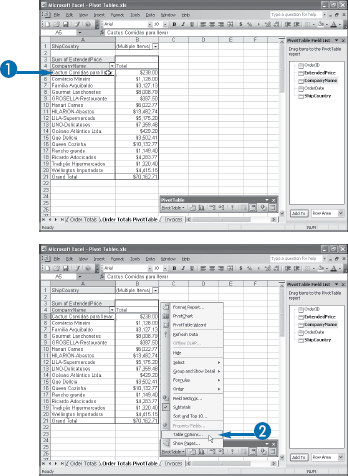
You can also right-click any PivotTable cell and then click Table Options.
The PivotTable Options dialog box appears.

Excel recalculates the PivotTable to include the hidden page items.