A PivotTable is a powerful data analysis tool because it can take hundreds or even thousands of records and summarize them into a compact, comprehensible report. However, unlike most of Excel's other data analysis features, a PivotTable is not a static collection of worksheet cells. Instead, you can move a PivotTable's fields from one area of the PivotTable to another. This enables you to view your data from different perspectives, which can greatly enhance the analysis of the data. Moving a field within a PivotTable is called pivoting the data.

The most common way to pivot the data is to move fields between the row and column areas. If your PivotTable contains just a single non-data field, moving the field between the row and column areas changes the orientation of the PivotTable between horizontal (column area) and vertical (row area). If your PivotTable contains fields in both the row and column areas, pivoting one of those fields to the other area creates multiple fields in that area. For example, pivoting a field from the column area to the row area creates two fields in the row area. This changes how the data breaks down, as described in Chapter 3; see the task "Add Multiple Fields to the Row or Column Area."

You can also pivot data by moving a row or column field to the page area, and a page field to the row or column area. This is a useful technique when you want to turn one of your existing row or column fields into a filter; see the next task, "Display a Different Page."

Move a Field to a Different Area

MOVE A FIELD BETWEEN THE ROW AND COLUMN AREAS

Note

This chapter uses the PivotTables.xls spreadsheet, available at www.wiley.com/go/pivottablesvb, or you can create your own sample database.

You can also drag a field button from the row area and drop it within the column area.

MOVE A ROW OR COLUMN FIELD TO THE PAGE AREA

Note

You must display the PivotTable Field List to move a field into the page area. When the PivotTable Field List is hidden, Excel does not show the page area if it is empty.

You can also drag a field button from the column area and drop it within the page area.

Apply It

You can also move any row, column, or page area field to the PivotTable's data area. This may seem strange because row, column, and page fields are almost always text values, and the default data area calculation is Sum. How can you sum text values? You cannot, of course. Instead, Excel's default PivotTable summary calculation for text values is Count. So, for example, if you drag the Category field and drop it inside the data area, Excel creates a second data field named Count of Category. To learn more about working with multiple data area fields, see the Chapter 3 task, "Add Multiple Fields to the Data Area."

As you move fields within the PivotTable, Excel changes the mouse pointer depending on the PivotTable area over which the pointer is hovering:

Button	Description
	Mouse pointer for the row area.
	Mouse pointer for the column area.
	Mouse pointer for the data area.
	Mouse pointer for the page area.

By default, each PivotTable report displays a summary for all the records in your source data. This is usually what you will want to see. However, there may be situations in which you need to focus more closely on some aspect of the data. You can focus in on a specific item from one of the source data fields by taking advantage of the PivotTable's page field.

For example, suppose you are dealing with a PivotTable that summarizes data from thousands of customer invoices over some period of time. A basic PivotTable might tell you the total amount sold for each product that you carry. That is interesting, but what about if you want to see the total amount sold for each product in a specific country. If the Product field is in the PivotTable's row area, then you could add the Country field to the column area. However, there may be dozens of countries, so that is not an efficient solution. Instead, you could add the Country field to the page area. You can then tell Excel to display the total sold for each product for the specific country in which you are interested.

As another example, suppose you ran a marketing campaign in the previous quarter and you set up an incentive plan for your salespeople whereby they could earn bonuses for selling at least a specified number of units. Suppose, as well, that you have a PivotTable showing the sum of the units sold for each product. To see the numbers for a particular employee, you could add the Salesperson field to the page area, and then select the employee you want to work with.

Display a Different Page

Excel displays a list of the page field values.

Excel filters the PivotTable to show only the data for the page you selected.

DISPLAY ALL PAGES

Excel displays a list of the page field values.

Excel adjusts the PivotTable to show the data for all the pages.

Apply It

You can add multiple fields to the page area, as described in the Chapter 3 task "Add Multiple Fields to the Page Area." This enables you to apply multiple filters to the data. For example, suppose you have a PivotTable that summarizes invoice data by showing the total amount sold for each product that you carry, and that you have a page field with Country data that enables you to isolate the sales by product for a specific country. You might then want to extend your analysis to look at the country-specific sales by product for individual salespersons.

To do this, you would add the Salesperson field as a second field in the page area. You could then use the steps shown in this task to choose a specific country and a specific salesperson. Remember that it does not matter which order the fields appear in the page area, because the filtering comes out the same in the end.

When you filter your PivotTables using multiple page fields, be aware that not all combinations of items from the fields will produce PivotTable results. For example, a particular salesperson may not have sold any products to customers in a specific country, so combining those filters produces a PivotTable without any data.

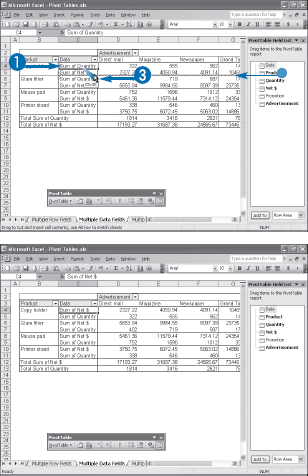
You learned in the Chapter 3 task "Add Multiple Fields to the Row or Column Area," that you can add two or more fields to any area in the PivotTable. This enables you to break down the data in different ways (multiple row or column area fields), apply extra filters (multiple page area fields), or display extra summaries (multiple data area fields). After you have multiple fields in an area, Excel allows you to change the order of those fields to reconfigure your data the way you prefer. This is another example of pivoting the data.

How you pivot within a field depends on the field. For row, column, and page fields, you pivot by dragging and dropping field buttons within the same area. For example, if the row area of the PivotTable has the Product field on the outside (left) and the Promotion field on the inside (right), the PivotTable shows the sales of each product broken down by the promotion. If, instead, you prefer to see the sales of each promotion broken down by product, then you need to switch the order of the Product and Promotion fields.

If you have multiple data fields, on the other hand, Excel does not display a button for each field. In this case, you change the order of the data area fields by dragging and dropping any data field label. Note, however, that this does not change the data summaries themselves, just the order in which they appear in the PivotTable.

Change the Order of Fields Within an Area

CHANGE THE FIELD ORDER IN THE ROW, COLUMN, OR PAGE AREA

Excel reconfigures the PivotTable.

CHANGE THE FIELD ORDER IN THE DATA AREA

Excel reconfigures the PivotTable.

Apply It

The most common situation for changing field order is to move a row field to the outer position. Here is a VBA macro that automates this process:

Sub SwitchRowFields()
    Dim objPT As PivotTable
    Dim objPTField As PivotField
    ' Work with the first PivotTable on the active worksheet
    Set objPT = ActiveSheet.PivotTables(1)
    With objPT
        ' If there is just one row field, exit
        If .RowFields.Count = 1 Then Exit Sub
        ' Run through all the row fields
        For Each objPTField In .RowFields
            ' Is the current field the innermost field?
            If objPTField.Position = .RowFields.Count Then
                ' If so, make it the outer field
                objPTField.Position = 1
                ' We are done, so exit
                Exit Sub
            End If
        Next 'objPTField
    End With
End Sub

When you create a PivotTable, Excel sorts the data in ascending order based on the items in the row and column fields. For example, if the row area contains the Product field, the vertical sort order of the PivotTable is ascending according to the items in the Product field. You can change this default sort order to one that suits your needs. Excel gives you two choices: you can switch between ascending and descending, or you can sort based on a data field instead of a row or column field.

Changing the sort order often comes in handy when you are working with dates or times. The default ascending sort shows the oldest items at the top of the field; if, instead, you are more interested in the most recent items, switch to a descending sort to show those items at the top of the field.

Sorting the PivotTable based on the values in a data field is useful when you want to rank the results. For example, if your PivotTable shows the sum of sales for each product, an ascending or descending sort of the product name enables you to easily find a particular product. However, if you are more interested in finding which products sold the most (or the least), then you need to sort the PivotTable on the data field.

Excel gives you two methods for sorting PivotTable items: you can have Excel sort the items automatically using the AutoSort feature, as you learn in this task; alternatively, you can create a custom sort order by manually adjusting the items; see the next task, "Move Row and Column Items."

Sort PivotTable Data with AutoSort

Excel displays the PivotTable Sort and Top 10 dialog box.

Excel sorts the PivotTable.

Extra

In Excel, an ascending sort means that items are arranged in the following order: numbers, text, logical values, error values (such as #REF! and #N/A), and blank cells. A descending sort reverses this order, except for blank cells: error values (such as #REF! and #N/A), logical values, text, numbers, and blank cells.

You can also sort a PivotTable using Excel's Sort feature. Click any cell in the field that you want to use for sorting: for a row or column field, click either the field button or any item within the field; for the data field, click the label or any data value within the field. Click Data→Sort to display the Sort dialog box. Select Ascending or Descending (

To return the PivotTable to the default sort order, follow Steps 1 and 2 to display the PivotTable Sort and Top 10 dialog box. Select Manual (

As you saw in the previous task, Excel's AutoSort feature enables you to apply an ascending or descending sort on a row or column field, or on a data item. However, there may be situations where these basic sort options do not fit your requirements. In these cases, you can solve the problem by coming up with a custom sort order, and Excel offers a couple of methods for doing just that.

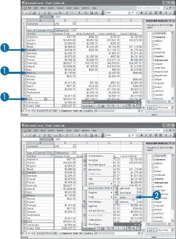
For example, suppose you have a PivotTable that shows the sales generated by each employee, broken down by country. Showing the Country field items alphabetically makes sense in most situations, but suppose you are preparing the report for managers who oversee the sales on each continent (North America, South America, Europe, and so on). In this case, it would be more convenient for those managers if you organized the PivotTable countries by continent. However, because there is no "continent" field to sort on, you need to sort the countries by hand.

To sort a PivotTable by hand, you need to move the row or column items individually. As you learn in this task, you can move individual row or column items either by using commands on the PivotTable toolbar, or by using your mouse to click and drag the items.

Move Row and Column Items

USE COMMANDS TO MOVE ROW AND COLUMN ITEMS

Excel displays a submenu of commands for moving the item.

Excel moves the item.

Click and Drag to Move Row and Column Items

Apply It

Excel offers a third method for moving row and column items to apply a custom sort order, and this method uses a rather surprising trick. To move a particular row or column item, first click the row or column item that is currently in the position where you want the moved item to end up. For example, if you want to move the item to the top of the items in the row area, click the first item in the row area. Now type the text of the item you want Excel to move. For example, if the item you want to move is "Brazil," type Brazil. When you press Enter to confirm the typing, Excel switches the two items. That is, Excel moves the item you typed to the current cell, and Excel moves the item that was previously in the cell to the cell where the moved item used to appear.

What makes this technique even more convenient is that Excel monitors your typing and its AutoComplete feature should fill in the text of the item you want to move after just a few keystrokes. For example, after you type Br, Excel should fill in Brazil automatically.

By default, your PivotTable shows all the items in whatever row and column fields you added to the report layout. This is usually what you want because the point of a PivotTable is to summarize all the data in the original source. However, you may not always want to see every item. In particular, you may only be interested in the top 10 items. You can generate such a report by using Excel's Top 10 AutoShow feature, which shows just the top 10 items, based on the values in the data field.

For example, suppose you have a PivotTable report based on a database of invoices that shows the total sales for each product. The basic report shows all the products, but if you are only interested in the top performers for the year, you can activate the Top 10 AutoShow feature to see the 10 products that sold the most.

Despite its name, the Top 10 AutoShow feature can display more than just the top 10 data values. You can specify any number between 1 and 255, and you can also ask Excel to show the bottommost values.

Show Only the Top 10 Items

Excel displays the PivotTable Sort and Top 10 dialog box.

Excel displays the top 10 values for the field.

Note

To display all the items again, follow Steps 1 and 2, select Off, and then click OK.

Apply It

Here is a VBA script that activates the Top 10 AutoShow feature. If you want to create a script that deactivates this features, copy the script — making sure to change the procedure name, too — and in the AutoShow statement, replace xlAutomatic with xlManual.

Example:

Sub ActivateTop10AutoShow()
    Dim objPT As PivotTable
    Dim objPTRowField As PivotField
    Dim strDataFieldName As String
    '
    ' Work with the first PivotTable on the active worksheet
    Set objPT = ActiveSheet.PivotTables(1)
    '
    ' Work with the first row field
    Set objPTRowField = objPT.RowFields(1)
    '
    ' Get the data field name
    strDataFieldName = objPT.DataFields(1).Name
    '
    ' Set the Top 10 AutoShow
    objPTRowField.AutoShow xlAutomatic, xlTop, 10, strDataFieldName
End Sub

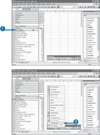
When you view a PivotTable report, it may contain items in a row or column field that you do not need to see. For example, in a report showing employee sales or other data, you may prefer to see only those employees that work for or with you. Similarly, if you are a product manager, you might want to customize the report to show only those items in the Product field that you are responsible for.

If you have a PivotTable that contains row or column items you do not need or want to see, you can remove those items from the report. Excel enables you to change the PivotTable view to exclude one or more items in any row or column field. After you have hidden the items, Excel reconfigures the report to display without them, and also updates the totals to reflect the excluded items. Note, too, that the items remain hidden even if you update the PivotTable, move the field to a different area, and even if you delete the field and add it back into the PivotTable.

After you have hidden one or more items, you should also know how to show them again. See the next task, "Show Hidden Items in a Row or Column Field."

Hide Items in a Row or Column Field

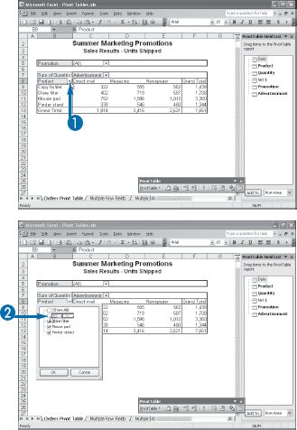
Excel displays a list of the items in the field.

Excel hides the items and reconfigures the PivotTable.

Extra

If you only want to hide a single item in a row or column field, Excel offers a more direct method: right-click the item and then click Hide. Note, however, that there is no similarly straightforward method for showing the item again. You must use the technique outlined in the next task, "Show Hidden Items in a Row or Column Field."

On the other hand, if your field has a large number of items, you may only want to show one or two of those items. Fortunately, there is a way to avoid deactivating all those check boxes. Deselect Show All (

In the previous task, you learned how to adjust the PivotTable view by hiding one or more items in any row or column field. The opposite case is when you have one or more hidden items and you wish to show some or all of them again. For example, if you have hidden product items that are outside your division, you might want to show products from other divisions that are comparable to one or more of yours. This enables you to use the PivotTable report to compare product results between divisions.

As you see in this task, the procedure for showing hidden items is the opposite of the procedure you used to hide them in the first place.

Show Hidden Items in a Row or Column Field

Excel displays a list of the items in the field.

Excel shows the items and reconfigures the PivotTable.

Apply It

Here is a VBA macro that shows all the hidden items in a PivotTable row and column areas:

Example:

Sub ShowAllItems()
    Dim objPT As PivotTable, objPTField As PivotField
    Dim objPTItem As PivotItem
    Set objPT = ActiveSheet.PivotTables(1)
        ' Run through all the row fields
        For Each objPTField In objPT.RowFields
            ' Get the hidden items and make them visible
            For Each objPTItem In objPTField.HiddenItems
                objPTItem.Visible = True
            Next 'objPTItem
        Next 'objPTField
        ' Run through all the column fields
        For Each objPTField In objPT.ColumnFields
            ' Get the hidden items and make them visible
            For Each objPTItem In objPTField.HiddenItems
                objPTItem.Visible = True
            Next 'objPTItem
        Next 'objPTField
End Sub

You use a page area field to act as a filter for your PivotTable data. When you select a page field item, Excel filters the PivotTable to show just the results for records that include the page item. See the task "Display a Different Page," earlier in this chapter, for details on changing PivotTable pages. This is most often useful when you want to see just a subset of data, but it can also come in handy when you want to compare the PivotTable results for two or more subsets. You configure the PivotTable for one page field item, view the results, and then repeat with a different page field item. This method works, but it is usually more efficient to compare two different PivotTables rather than switching the page items back and forth.

You can solve this problem by creating another PivotTable, but creating a replica of your PivotTable might be quite a bit of work, particularly if you are working with several pages — each of which would require its own PivotTable. Instead, Excel offers a Show Pages feature that, with just a few mouse clicks, enables you to create separate PivotTables that show the results for each item in a page field. Excel creates copies of your PivotTable in separate worksheets, one for each item in the page field. This enables you to compare the results by switching from one worksheet to another.

Show Pages as Worksheets

You can also click the Show Pages button (

Excel displays the Show Pages dialog box.

Apply It

If you find yourself using the Show Pages feature frequently, you may also find that you often have to delete the resulting worksheets. To help you automate this chore, here is a VBA macro that deletes the worksheets created by Show Pages:

Example:

Sub DeletePages()
    Dim objPT As PivotTable
    Dim objPageField As PivotField
    Dim objItem As PivotItem
    Dim strPageName As String
    ' Work with the first PivotTable on the active worksheet
    Set objPT = ActiveSheet.PivotTables(1)
    ' Work with the first page field
    Set objPageField = objPT.PageFields(1)
    ' Run through the page field items
    For Each objItem In objPageField.PivotItems
        ' Get the item value
        strPageName = objItem.Value
        ' Delete the corresponding worksheet
        ActiveWorkbook.Worksheets(strPageName).Delete
    Next 'objItem
End Sub

Most PivotTable reports have just a few items in the row and column fields, which makes the report easy to read and analyze. However, it is not unusual to have row or column fields that consist of dozens of items, which makes the report much harder to work with. One solution is to cut the report down to size by hiding items; see the task "Hide Items in a Row or Column Field," earlier in this chapter. Unfortunately, this solution is not appropriate if you need to work with all the PivotTable data.

To make a report with a large number of row or column items easier to work with, you can group the items together. For example, you could group months into quarters, thus reducing the number of items from 12 to 4. Similarly, a report that lists dozens of countries could group those countries by continent, thus reducing the number of items to 4 or 5, depending on where the countries are located. Finally, if you use a numeric field in the row or column area, you may have hundreds of items, one for each numeric value. You can improve the report by creating just a few numeric ranges.

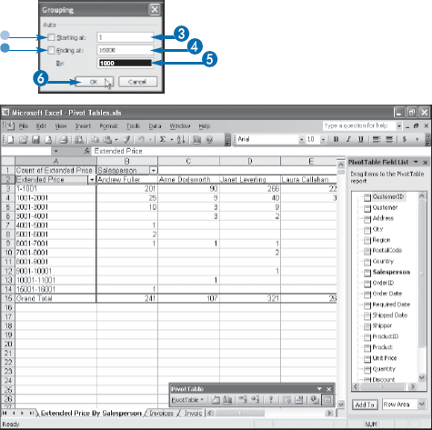
Excel enables you to group three types of data: numeric (discussed in this section), date and time (see "Group Date and Time Values"), and text (see "Group Text Values"). Grouping numeric values is useful when you use a numeric field in a row or column field. Excel enables you to specify numeric ranges into which the field items are grouped. For example, suppose you have a PivotTable of invoice data that shows the extended price (the row field) and the salesperson (the column field). It would be useful to group the extended prices into ranges and then count the number of invoices each salesperson processed in each range.

Group Numeric Values

You can also click the Group button (

The Grouping dialog box appears.

Excel groups the numeric values.

Extra

The ranges that Excel creates after you apply the grouping to a numeric field are not themselves numeric values; they are, instead, text values. Unfortunately, this means it is not possible to use Excel's AutoSort feature to switch the ranges from ascending order to descending order; see the task "Sort PivotTable Data with AutoSort," earlier in this chapter. If you try, Excel sorts the ranges as text, which usually results in improper sort orders. For example, in a descending sort, the range 2001–3001 would come before the range 10001–11001 because 2 (the first character of the text "2001–3001") has a higher value than 1 (the first character of the text "10001–11001"). To sort the ranges, you must move the items by hand. See the task "Move Row and Column Items," earlier in this chapter.

Similarly, the text nature of the range items means that you also cannot use Excel's Top 10 AutoShow feature, which only works properly with numeric values. See the task "Show Only the Top 10 Items," earlier in this chapter. The only way to simulate this feature would be to hide those ranges you do not want to view in your report; see the task "Hide Items in a Row or Column Field," earlier in this chapter.

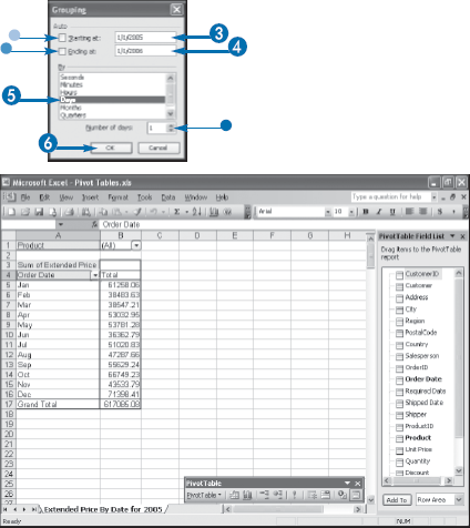
If your PivotTable includes a field with date or time data, you can use Excel's grouping feature to consolidate that data into more manageable or useful groups.

For example, a PivotTable based on a list of invoice data might show the total dollar amount, which is the Sum of Extended Price in the date area, of the orders placed on each day, which is the Date field in the row area. Tracking daily sales is useful, but a manager might need a report that shows the bigger picture. In that case, you can use the Grouping feature to consolidate the dates into weeks, months, or even quarters. Excel even allows you to choose multiple date groupings. For example, if you have several years' worth of invoice data, you could group the data into years, the years into quarters, and the quarters into months.

Excel also enables you to group time data. For example, suppose you have data that shows the time of day that an assembly line completes each operation. If you want to analyze how the time of day affects productivity, you could set up a PivotTable that groups the data into minutes — for example, 30-minute intervals — or hours.

Group Date and Time Values

You can also click the Group button (

The Grouping dialog box appears.

To use multiple groupings, click each type of grouping you want to use.

Excel groups the date or time values.

Apply It

In a factory or other manufacturing facility, it is often useful to analyze how productivity varies according to the day of the week. For example, which day of the week is the most productive? Which day is the least productive? Unfortunately, Excel does not have a "weekday" grouping type. To work around this limitation, create a new field in your source data and give it the heading Weekday. To derive the weekday for a given day, start with Excel's WEEKDAY() function, which returns a number from 1 to 7, where 1 corresponds to Sunday and 7 corresponds to Saturday. To convert the WEEKDAY() result into the day of the week, use the CHOOSE() function. If the cell with the date value is A1, use the following formula to derive the corresponding day of the week:

Example:

=CHOOSE(WEEKDAY(A1),"Sunday","Monday","Tuesday","Wednesday","Thursday","Friday", "Saturday")

When you have filled this formula for all the dates in your source data, build a new PivotTable and use the Weekday field in the row or column area. Excel will automatically consolidate the Weekday items into the days of the week.

You can use Excel's PivotTable Grouping feature to create custom groups from the text items in a row or column field.

One common problem that arises when you work with PivotTables is that you often need to consolidate items, but you have no corresponding field in the data. For example, the data may have a Country field, but what if you need to consolidate the PivotTable results by continent? It is unlikely that your source data includes a "Continent" field. Similarly, your source data may include employee names, but you may need to consolidate the employees according to the people they report to. What do you do if your source data does not include a "Supervisor" field?

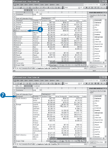
The solution in both cases is to use the Grouping feature to create custom groups. For the country data, you could create custom groups named "North America," "South America," "Europe," and so on. For the employees, you could create a custom group for each supervisor. You select the items that you want to include in a particular group, create the custom group, and then change the new group name to reflect its content. This task shows you the steps to follow to create such a custom grouping for text values.

Group Text Values

To select multiple cells in Excel, click the first cell, hold down Ctrl, and then click each of the other cells.

You can also click the Group button (

Excel creates a new group named Groupn (where n means this is the nth group you have created) and restructures the PivotTable.

Excel renames the group.

Extra

By default, Excel does not add subtotals to the bottom of each custom group. To add the subtotals, click any cell within the custom group, and then click PivotTable→Field Settings or click

Note, as well, that the values in the custom grouping — the group names — act as regular PivotTable text items. This means you can sort the groups either by applying an AutoSort or by moving the items by hand; see the tasks "Sort PivotTable Data with AutoSort" and "Move Row and Column Items," earlier in this chapter. You can also filter the items to hide or show only specific groups, as seen in the task "Hide Items in a Row or Column Field," earlier in this chapter.

When you consolidate a row or column field into groups, Excel reconfigures the PivotTable. For example, when you group a row field, Excel reconfigures the PivotTable to show two row fields: the groups appear in the outer row field and the items that comprise each group appear in the inner row field. The latter are called the group details. To make your report easier to read or manage, you can hide the details for a specific group. In this case, Excel collapses the group to a single line and displays just the group name and, in the data area, the group's subtotals. You can quickly toggle between hiding a group's details and showing them. For the latter, see the next task, "Show Group Details."

The following VBA macro hides the details for all the groups in a PivotTable's row area:

Example:

Sub HideAllGroupDetails()
    Dim objPT As PivotTable
    Dim objRowField As PivotField
    Dim objItem As PivotItem
    '
    ' Work with the first PivotTable on the active worksheet
    Set objPT = ActiveSheet.PivotTables(1)
    '
    ' Work with the outermost row field
    Set objRowField = objPT.RowFields(objPT.RowFields.Count)
    '
    ' Hide the details for each item
    For Each objItem In objRowField.PivotItems
        objItem.ShowDetail = False
    Next 'objItem
End Sub

Hide Group Details

You can also click the Hide Detail button (

Excel hides the group's details.

If you have hidden the details for a group using the Hide Detail command — see the previous task, "Hide Group Details" — you can use the Show Detail command to redisplay the group's details. This enables you to quickly and easily display whatever level of detail you prefer in a PivotTable report.

The following VBA macro shows the details for all the groups in a PivotTable's row area:

Example:

Sub ShowAllGroupDetails()
    Dim objPT As PivotTable
    Dim objRowField As PivotField
    Dim objItem As PivotItem
    '
    ' Work with the first PivotTable on the active worksheet
    Set objPT = ActiveSheet.PivotTables(1)
    '
    ' Work with the outermost row field
    Set objRowField = objPT.RowFields(objPT.RowFields.Count)
    '
    ' Hide the details for each item
    For Each objItem In objRowField.PivotItems
        objItem.ShowDetail = True
    Next 'objItem
End Sub

Show Group Details

You can also click the Show Detail button (

Excel shows the group's details.

Grouping is a very useful PivotTable feature and you will likely find that you make groups a permanent part of many of your PivotTables. On the other hand, you can also use grouping as a temporary data analysis tool. That is, you build your PivotTable, organize a field into groups, and then analyze the results. At this point, if you no longer need the groupings, then you need to reverse the process. With Excel's Ungroup command, you can remove the groupings from your PivotTable.

Excel gives you two ways to use the Ungroup command. The most common method is to use the command to ungroup all the values in the row or column area, thus returning the PivotTable to its normal layout. However, if you are working with text groupings, as seen in "Group Text Values," Excel also enables you to ungroup a single grouping of values, while leaving the other text groupings intact. In this case, Excel displays the group values in both the outer and the inner fields. This can be a bit confusing, so you should only use this technique on occasion.

Ungroup Values

UNGROUP ALL VALUES

You can also click the Ungroup button (

Excel ungroups all the values.

UNGROUP A TEXT GROUPING

You can also click the Ungroup button (

Excel ungroups all the values in the text grouping.

Apply It

Here is a VBA macro that ungroups the row values in a PivotTable:

Example:

Sub UngroupAll()
    Dim objPT As PivotTable
    Dim objRowField As PivotField
    Dim objItem As PivotItem
    '
    ' Work with the first PivotTable on the active worksheet
    Set objPT = ActiveSheet.PivotTables(1)
    '
    ' Work with the outermost row field
    Set objRowField = objPT.RowFields(objPT.RowFields.Count)
    '
    ' Select the row
    objPT.PivotSelect objRowField.Name & "[All]"
    '
    ' Ungroup it
    Selection.Ungroup
End Sub

In Chapter 3, you learned how to add multiple fields to the PivotTable's page area; see the task "Add Multiple Fields to the Page Area." When you add a second field to the page area, Excel displays one field below the other, which is the basic page area layout. However, many PivotTable applications require a large number of page area fields, sometimes half a dozen or more. By default, Excel displays these fields vertically, one on top of another. You can alter this default configuration by changing the page area layout to one that suits the layout of the rest of the PivotTable.

Excel gives you two ways to change the page area layout. The most basic change is to reconfigure how the page area fields appear on the worksheet. The default is vertically (one on top of another), but you can also change the fields to appear horizontally (one beside another).

After you have selected the basic orientation, you can then change whether Excel displays the fields in multiple columns or rows. For example, if you choose the vertical orientation (Excel calls it Down, Then Over), you can also specify the number of fields that appear in each column. If you have, say, six page fields and you specify two columns, Excel displays the first three fields in one column and the other three fields in the next column. Similarly, if you choose the horizontal orientation (called Over, Then Down), you can also specify the number of fields that appear in each row.

Change the Page Area Layout

The PivotTable Options dialog box appears.

Click

If you select the Down, Then Over page layout in Step 3, specify the maximum number of fields that you want Excel to display in each column.

Note

If you enter 0 in the Fields per row (or Fields per column) box, Excel displays the page fields in a single row (or column).

Excel reconfigures the layout of the page area.

Apply It

If you want to use VBA to control the page area layout, the PivotTable object has two properties you can work with: PageFieldOrder and PageFieldWrapCount. Use the PageFieldOrder property to set the page area orientation (to either xlDownThenOver or xlOverThenDown); and use the PageFieldWrapCount property to set the number of rows or columns you want in the page area layout. The following code sets these properties for a PivotTable object:

Example:

Set objPT = ActiveSheet.PivotTables(1)
With objPT
    .PageFieldOrder = xlOverThenDown
    .PageFieldWrapCount = 2
End With