2
DSP Basics
2.1 Introduction
In the early days of electronics, signals were processed and transmitted in their natural form, typically an analogue signal created from a source signal such as speech, then converted to electrical signals before being transmitted across a suitable transmission medium such as a broadband connection. The appeal of processing signals digitally was recognized quite some time ago for a number of reasons. Digital hardware is generally superior and more reliable than its analogue counterpart, which can be prone to aging and can give uncertain performance in production.
DSP, on the other hand, gives a guaranteed accuracy and essentially perfect reproducibility (Rabiner and Gold 1975). In addition, there is considerable interest in merging the multiple networks that transmit these signals, such as the telephone transmission networks, terrestrial TV networks and computer networks, into a single or multiple digital transmission media. This provides a strong motivation to convert a wide range of information formats into their digital formats.
Microprocessors, DSP microprocessors and FPGAs are a suitable platform for processing such digital signals, but it is vital to understand a number of basic issues with implementing DSP algorithms on, in this case, FPGA platforms. These issues range from understanding both the sampling rates and computation rates of different applications with the aim of understanding how these requirements affect the final FPGA implementation, right through to the number representation chosen for the specific FPGA platform and how these decisions impact the performance. The choice of algorithm and arithmetic requirements can have severe implications for the quality of the final implementation.
As the main concern of this book is the implementation of such systems in FPGA hardware, this chapter aims to give the reader an introduction to DSP algorithms to such a level as to provide grounding for many of the examples that are described later. A number of more extensive introductory texts that explain the background of DSP systems can be found in the literature, ranging from the basic principles (Lynn and Fuerst 1994; Williams 1986) to more comprehensive texts (Rabiner and Gold 1975).
Section 2.2 gives an introduction to basic DSP concepts that affect hardware implementation. A brief description of common DSP algorithms is then given, starting with a review of transforms, including the FFT, discrete cosine transform (DCT) and the discrete wavelet transform (DWT) in Section 2.3. The chapter then moves on to review filtering in Section 2.4, giving a brief description of finite impulse response (FIR) filters, infinite impulse response (IIR) filters and wave digital filters (WDFs). Section 2.5 is dedicated to adaptive filters and covers both the least mean squares (LMS) and recursive least squares (RLS) algorithms. Concluding comments are given in Section 2.6.
2.2 Definition of DSP Systems
DSP algorithms accept inputs from real-world digitized signals such as voice, audio, video and sensor data (temperature, humidity), and mathematically process them according to the required algorithm’s processing needs. A simple diagram of this process is given in Figure 2.1. Given that we are living in a digital age, there is a constantly increasing need to process more data in the fastest way possible.
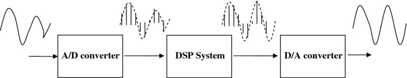
Figure 2.1 Basic DSP system
The digitized signal is obtained as shown in Figure 2.2 where an analogue signal is converted into a pulse of signals and then quantized to a range of values. The input is typically ![]() , which is a stream of numbers in digital format, and the output is given as
, which is a stream of numbers in digital format, and the output is given as ![]() .
.
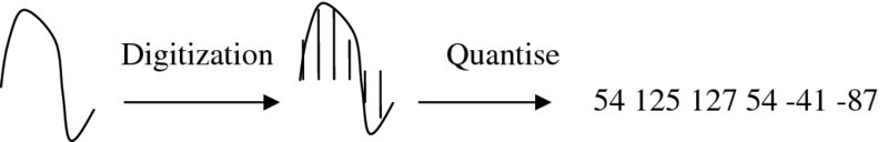
Figure 2.2 Digitization of analogue signals
Modern DSP applications mainly involve speech, audio, image, video and communications systems, as well as error detection and correction and encryption algorithms. This involves real-time processing of a considerable amount of different types of content at a series of sampling rates ranging from 1 Hz in biomedical applications, right up to tens of megahertz in image processing applications. In a lot of cases, the aim is to process the data to enhance part of the signal (e.g. edge detection in image processing), eliminate interference (e.g. jamming signals in radar applications), or remove erroneous input (e.g. echo or noise cancelation in telephony); other DSP algorithms are essential in capturing, storing and transmitting data, audio, images, and video compression techniques have been used successfully in digital broadcasting and telecommunications.
Over the years, much of the need for such processing has been standardized; Figure 2.3 shows some of the algorithms required in a range of applications. In communications, the need to provide efficient transmission using orthogonal frequency division multiplexing (OFDM) has emphasized the need for circuits for performing FFTs. In image compression, the evolution initially of the Joint Photographic Experts Group (JPEG) and then the Motion Picture Experts Group (MPEG) led to the development of the JPEG and MPEG standards respectively involving a number of core DSP algorithms, specifically DCT and motion estimation and compensation.
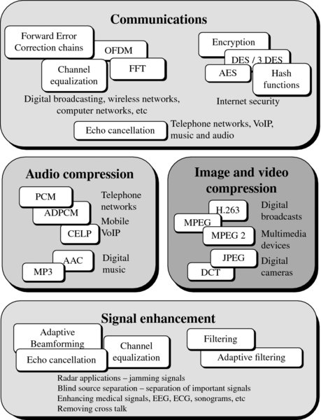
Figure 2.3 Example applications for DSP
The appeal of processing signals digitally was recognized quite some time ago as digital hardware is generally superior to and more reliable than its analogue counterpart; analogue hardware can be prone to aging and can give uncertain performance in production. DSP, on the other hand, gives a guaranteed accuracy and essentially perfect reproducibility (Rabiner and Gold 1975).
The proliferation of DSP technology has mainly been driven by the availability of increasingly cheap hardware, allowing the system to be easily interfaced to computer technology, and in many cases, to be implemented on the same computers. The need for many of the applications mentioned in Figure 2.3 has driven the need for increasingly complex DSP systems, which in turn has seen the growth of research into developing efficient implementation of some DSP algorithms. This has also driven the need for DSP microprocessors covered in Chapter 4.
A number of different DSP functions can be carried out either in the time domain, such as filtering, or in the frequency domain by performing an FFT (Rabiner and Gold 1975). The DCT forms the central mechanism for JPEG image compression which is also the foundation for the MPEG standards. This DCT algorithm enables the components within the image that are invisible to the naked eye to be identified by converting the spatial image into the frequency domain. They can then be removed using quantization in the MPEG standard without discernible degradation in the overall image quality. By increasing the amount of data removed, greater reduction in file size can be achieved. Wavelet transforms offer both time domain and frequency domain information and have roles not only in applications for image compression, but also in extraction of key information from signals and for noise cancelation. One such example is in extracting key features from medical signals such as the electroencephalogram (EEG).
2.2.1 Sampling
Sampling is an essential process in DSP that allows real-life continuous-time domain signals, in other words analogue signals, to be represented in the digital domain. The process of representation of analogue signals process begins with sampling and is followed by the quantization within the analogue-to-digital converters (ADCs). Therefore, the two most important components in the sampling process are the selection of the samples in time domain and subsequent quantization of the samples within the ADC, which results in quantization noise being added to the digitized analogue signal. The choice of sampling frequency directly affects the size of data processed by the DSP system.
A continuous-time (analogue) signal can be converted into a discrete-time signal by sampling the continuous-time signal at uniformly distributed discrete-time instants. Sampling an analogue signal can be represented by the relation
where xa(nT) represents the uniformly sampled discrete-time signal. The data stream, x(n), is obtained by sampling the continuous-time signal at the required time interval, given as the sampling instance, T; this is called the sampling period or interval, and its reciprocal is called the sampling rate, Fs.
The question arises as to how precise the digital data need to be to have a meaningful representation of the analogue word. This definition is explained by the Nyquist–Shannon sampling theorem which states that exact reconstruction of a continuous-time baseband signal from its samples is possible if the signal is bandlimited and the sampling frequency is greater than twice the signal bandwidth. The sampling theory was introduced into communication theory by Nyquist (1928) and then into information theory by Shannon (1949).
2.2.2 Sampling Rate
Many computing vendors quote clock rates, whereas the rate of computation in DSP systems is given as the sampling rate. It is also important to delineate the throughput rate. The sampling rate for many typical DSP systems is given in Figure 2.4 and indicates the rate at which data are fed into and/or from the system. It should not be used to dictate technology choice as, for example, we could have a 128-tap FIR filter requirement for an audio application where the sampling rate may be 44.2 kHz but the throughput rate will be 11.2 megasamples per second (MSPS), as during each sample we need to compute 128 multiplications and 127 additions (255 operations) at the sampling rate.
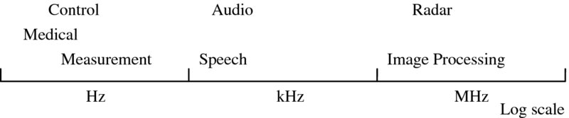
Figure 2.4 Sampling rates for many DSP systems
In simple terms when digitizing an analogue signal, the rate of sampling must be at least twice the maximum frequency fm (within the signal being digitized) so as to maintain the information and prevent aliasing (Shannon 1949). In other words, the signal needs to be bandlimited, meaning that there is no spectral energy above the maximum frequency fm. The Nyquist sampling rate fs is then determined as 2fm, usually by human factors (e.g. perception).
A simple example is the sampling of speech, which is standardized at 8 kHz. This sampling rate is sufficient to provide an accurate representation of the spectral components of speech signals, as the spectral energy above 4 kHz, and probably 3 kHz, does not contribute greatly to signal quality. In contrast, digitizing music typically requires a sample rate of 44.2 kHz to cover the spectral range of 22.1 kHz as it is acknowledged that this is more than sufficient to cope with the hearing range of the human ear which typically cannot detect signals above 18 kHz. Moreover, this increase is natural due to the more complex spectral composition of music when compared with speech.
In other applications, the determination of the sampling rate does not just come down to human perception, but involves other aspects. Take, for example, the digitizing of medical signals such as EEGs which are the result of electrical activity within the brain picked up from electrodes in contact with the surface of the skin. In capturing the information, the underlying waveforms can be heavily contaminated by noise. One particular application is a hearing test whereby a stimulus is applied to the subject’s ear and the resulting EEG signal is observed at a certain location on the scalp. This test is referred to as the auditory brainstem response (ABR) as it looks for an evoked response from the EEG in the brainstem region of the brain, within 10 ms of the stimulus onset.
The ABR waveform of interest has a frequency range of 100–3000 Hz, therefore bandpass filtering of the EEG signal to this region is performed during the recording process prior to digitization. However, there is a slow response roll-off at the boundaries and unwanted frequencies may still be present. Once digitized the EEG signal may be filtered again, possibly using wavelet denoising to remove the upper and lower contaminating frequencies. The duration of the ABR waveform of interest is 20 ms, 10 ms prior to stimulus and 10 ms afterward. The EEG is sampled at 20 kHz, therefore with a Nyquist frequency of 10 kHz, which exceeds twice the highest frequency component (3 kHz) present in the signal. This equates to 200 samples, before and after the stimulus.
2.3 DSP Transformations
This section gives a brief overview of some of the key DSP transforms mentioned in Chapter 13, including a brief description of applications and their use.
2.3.1 Discrete Fourier Transform
The Fourier transform is the transform of a signal from the time domain representation to the frequency domain representation. In basic terms it breaks a signal up into its constituent frequency components, representing a signal as the sum of a series of sines and cosines.
The Fourier series expansion of a periodic function, f(t), is given by
where, for any non-negative integer n, ωn is the nth harmonic in radians of f(t) given by
the an are the even Fourier coefficients of f(t), given by
and the bn are the odd Fourier coefficients, given by
The discrete Fourier transform (DFT), as the name suggests, is the discrete version of the continuous Fourier transform, applied to sampled signals. The input sequence is finite in duration and hence the DFT only evaluates the frequency components present in this portion of the signal. The inverse DFT will therefore only reconstruct using these frequencies and may not provide a complete reconstruction of the original signal (unless this signal is periodic).
The DFT converts a finite number of equally spaced samples of a function, to a finite list of complex sinusoids, where the transformation is ordered by frequency. This transformation is commonly described as transferring a sampled function from time domain to frequency domain. Given the N-point of equally spaced sampled function x(n) as an input, the N-point DFT is defined by
where n is the time index and k is the frequency index.
The compact version of the DFT can be written using the twiddle factor notation:
Using the twiddle factor notation, equation (2.7) can be written as follows:
The input sequence x(n) can be calculated from X(k) using the inverse discrete Fourier transform (IDFT) given by
The number of operations performed for one output can be easily calculated as N complex multiplications and N − 1 complex additions from equations (2.8) and (2.9). Therefore, the overall conversion process requires N2 complex multiplications and N2 − N complex additions. The amount of calculation required for an N-point DFT equation is approximately 2N2.
2.3.2 Fast Fourier Transform
In order to reduce the amount of mathematical operations, a family of efficient calculation algorithms called fast Fourier transforms was introduced by Cooley and Tukey (1965). The basic methodology behind the FFT is the computation of large DFTs in small pieces, and their combination with the help of reordering and transposition algorithms. At the end, the combined result gives the same values as with the large sized DFT, but the order of complexity of the main system reduces from N2 to the order of Nlog (N).
The transformed samples are separated by the angle θ and are periodic and mirrored to the left and right of the imaginary and above and below the real axis. This symmetry and periodicity in the coefficients of the transform kernel (WN) gives rise to a family of FFT algorithms which involves recursively decomposing the algorithm until only two-point DFTs are required. It is computed using the butterfly unit and perfect shuffle network as shown in Figure 2.5:
Figure 2.5 Eight-point radix-2 FFT structure
The FFT has immense impact in a range of applications. One particular use is in the central computation within OFDM. This spread spectrum digital modulation scheme is used in communication, particularly within wireless technology, and has resulted in vastly improved data rates within the 802.11 standards, to name just one example. The algorithm relies on the orthogonal nature of the frequency components extracted through the FFT, allowing each of these components to act as a sub-carrier. Note that the receiver uses the inverse fast Fourier transform (IFFT) to detect the sub-carriers and reconstruct the transmission. The individual sub-carriers are modulated using a typical low symbol rate modulation scheme such as phase-shift or quadrature amplitude modulation (QAM), depending on the application.
For the Institute of Electrical and Electronic Engineers (IEEE) 802.11 standard, the data rate ranges up to 54 Mbps depending on the environmental conditions and noise, i.e. phase shift modulation is used for the lower data rates when greater noise is present, and QAM is used in less noisy environments reaching up to 54 Mbps. Figure 2.6 gives an example of the main components within a typical communications chain.
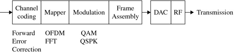
Figure 2.6 Wireless communications transmitter
The IEEE 802.11a wireless LAN standard using OFDM is employed in the 5 GHz region of the US ISM band over a channel bandwidth of 125 MHz. From this bandwidth 52 frequencies are used, 48 for data and four for synchronization. The latter point is very important, as the basis on which OFDM works (i.e. orthogonality) relies on the receiver and transmitter being perfectly synchronized.
2.3.3 Discrete Cosine Transform
The DCT is based on the DFT, but uses only real numbers, i.e. the cosine part of the transform, as defined in the equation
This two-dimensional (2D) form of the DCT is a vital computational component in the JPEG image compression and also features in MPEG standards:
where u is the horizontal spatial frequency for 0 ⩽ u < 8, v is the vertical spatial frequency for 0 ⩽ v < 8, α(u) and α(v) are constants, fx, y is the value of the (x, y) pixel and Fu, v is the value of the (u, v) DCT coefficient.
In JPEG image compression, the DCT is performed on the rows and the columns of the image block of 8 × 8 pixels. The resulting frequency decomposition places the more important lower-frequency components at the top left-hand corner of the matrix, and the frequency of the components increases when moving toward the bottom right-hand part of the matrix.
Once the image has been transformed into numerical values representing the frequency components, the higher frequency components may be removed through the process of quantization as they will have less importance in image quality. Naturally, the greater the amount to be removed the higher the compression ratio; at a certain point, the image quality will begin to deteriorate. This is referred to as lossy compression. The numerical values for the image are read in a zigzag fashion.
2.3.4 Wavelet Transform
A wavelet is a fast-decaying waveform containing oscillations. Wavelet decomposition is a powerful tool for multi-resolution filtering and analysis and is performed by correlating scaled versions of this original wavelet function (i.e. the mother wavelet) against the input signal. This decomposes the signal into frequency bands that maintain a level of temporal information (Mallat 1989). This is particularly useful for frequency analysis of waveforms that are pseudo-stationary where the time-invariant FFT may not provide the complete information.
There are many families of wavelet equations such as the Daubechies, Coiflet and Symmlet (Daubechies 1992). Wavelet decomposition may be performed in a number of ways, namely the continuous wavelet transform (CWT) or DWT which is described in the next section.
Discrete Wavelet Transform
The DWT is performed using a series of filters. At each stage of the DWT, the input signal is passed though a high-pass and a low-pass filter, resulting in the detail and approximation coefficients.
The equation for the low-pass filter is
where g denotes high-pass. By removing half the frequencies at each stage, the signal information can be represented using half the number of coefficients, hence the equations for the low and high filters become
and
respectively, where h denotes low-pass, and where n has become 2n, representing the down-sampling process.
Wavelet decomposition is a form of subband filtering and has many uses. By breaking the signal down into the frequency bands, denoising can be performed by eliminating the coefficients representing the highest frequency components and then reconstructing the signal using the remaining coefficients. Naturally, this could also be used for data compression in a similar way to the DCT and has been applied to image compression. Wavelet decomposition is also a powerful transform to use in analysis of medical signals.
2.4 Filters
Digital filtering is achieved by performing mathematical operations on the digitized data; in the analogue domain, filtering is performed with the help of electronic circuits that are formed from various electronic components. In most cases, a digital filter performs operations on the sampled signals with the use stored filter coefficients. With the use of additional components and increased complexity, digital filters could be more expensive than the equivalent analogue filters.
2.4.1 Finite Impulse Response Filter
A simple FIR filter is given by
where the ai are the coefficients needed to generate the necessary filtering response such as low-pass or high-pass and N is the number of filter taps contained in the function. The function can be represented using the classical signal flow graph (SFG) representation of Figure 2.7 for N = 3 given by
Figure 2.7 Original FIR filter SFG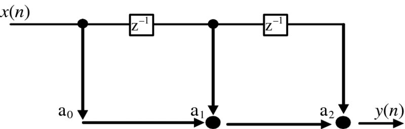
In the classic form, the delay boxes of z− 1 indicate a digital delay, the branches send the data to several output paths, labeled branches represent a multiplication by the variable shown and the black dots indicate summation functions. However, we find the form given in Figure 2.8 to be easier to understand and use this format throughput the book, as the functionality is more obvious than that given in Figure 2.7.

Figure 2.8 FIR filter SFG
An FIR filter exhibits some important properties including the following.
- Superposition. Superposition holds if a filter produces an output y(n) + v(n) from an input x(n) + u(n), where y(n) is the output produced from input x(n) and v(n) is the output produced from input u(n).
- Homogeneity. If a filter produces an output ay(n) from input ax(n) then the filter is said to be homogeneous if the filter produces an output ay(n) from input ax(n).
- Shift invariance. A filter is shift invariant if and only if the input of x(n + k) generates an output y(n + k), where y(n) is the output produced by x(n).
If a filter is said to exhibit all these properties then it is said to be a linear time-invariant (LTI) filter. This property allows these filters to be cascaded as shown in Figure 2.9(a) or in a parallel configuration as shown in Figure 2.9(b).
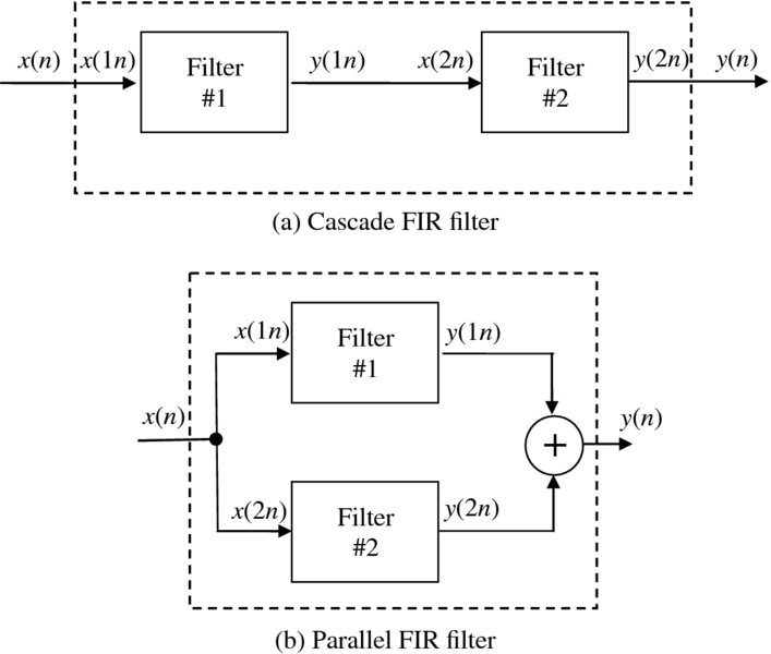
Figure 2.9 FIR filter configurations
FIR filters have a number of additional advantages, including linear phase, meaning that they delay the input signal but do not distort its phase; they are inherently stable; they are implementable using finite arithmetic; and they have low sensitivity to quantization errors.
Low-Pass FIR Filter
FIR filter implementations are relatively simple to understand as there is a straightforward relationship between the time and frequency domain. A brief summary is now given of digital filter design, but the reader is also referred to some good basic texts (Bourke 1999; Lynn and Fuerst 1994; Williams 1986) which give a much more comprehensive description of filter design. One basic way of developing a digital filter is to start with the desired frequency response, use an inverse filter to get the impulse response, truncate the impulse response and then window the function to remove artifacts (Bourke 1999; Williams 1986). The desired response is shown in Figure 2.10, including the key features that the designer wants to minimize.
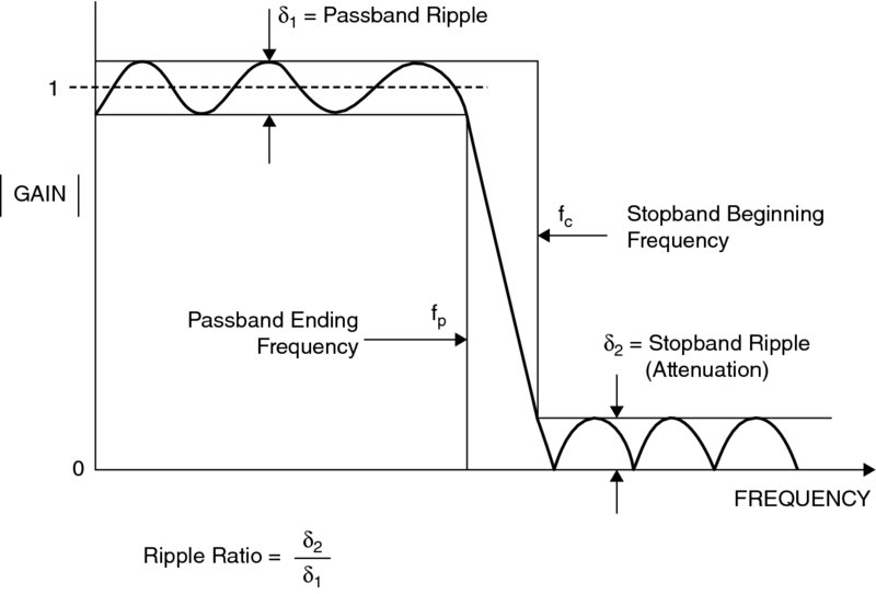
Figure 2.10 Filter specification features
Realistically we have to approximate this infinitely long filter with a finite number of coefficients and, given that it needs data from the future, time-shift it so that it does not have negative values. If we can then successfully design the filter and transform it back to the frequency domain we get a ringing in the passband/stopband frequency ranges known as rippling, a gradual transition between passband and stopband regions, termed the transition region. The ripple is often called the Gibbs phenomenon after Willard Gibbs who identified this effect in 1899, and it is outlined in the FIR filter response in Figure 2.10.
It could be viewed that this is the equivalent of windowing the original frequency plot with a rectangular window; there are other window types, most notably von Hann, Hamming and Kaiser windows (Lynn and Fuerst 1994; Williams 1986) that can be used to minimize these issues in different ways and to different levels. The result of the design process is the determination of the filter length and coefficient values which best meet the requirements of the filter response.
The number of coefficients has an impact on both the ripple and transition region and is shown for a low-pass filter design, created using the Hamming and Dolph–Chebyshev schemes in MATLAB®. The resulting frequency responses are shown in Figures 2.11 and 2.12 for 100 and 400, taps respectively. The impact of increasing the number of taps in the roll-off between the two bands and the reduction in ripple is clear.
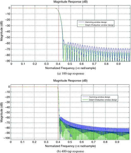
Figure 2.11 Low-pass filter response
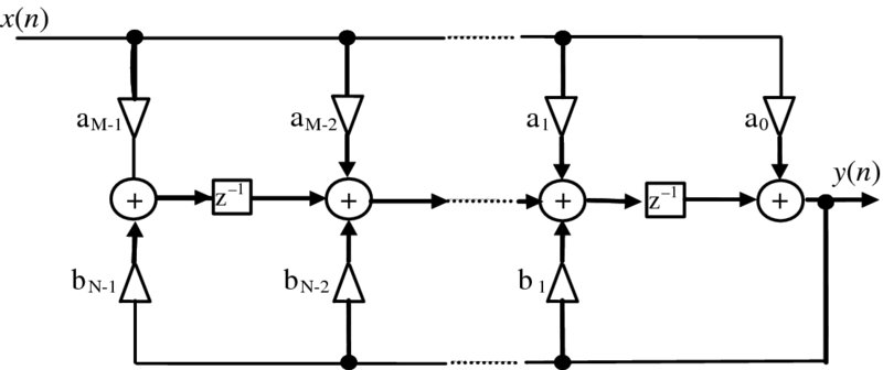
Figure 2.12 Direct form IIR filter
Increasing the number of coefficients clearly allows a better approximation of the filter but at the cost of the increased computation needed to compute the additional taps, and impacts the choice of windowing function.
2.4.2 Infinite Impulse Response filter
The main disadvantage of FIR filters is the large number of taps needed to realize some aspects of the frequency response, namely sharp cut-off resulting in a high computation cost to achieve this performance. This can be overcome by using IIR filters which use previous values of the output as indicated in the equation
This is best expressed in the transfer function expression
and is shown in Figure 2.12.
The design process is different from FIR filters and is usually achieved by exploiting the huge body of analogue filter designs by transforming the s-plane representation of the analogue filter into the z domain. A number of design techniques can be used such as the impulse invariant method, the match z-transform and the bilinear transform. Given an analogue filter with a transfer function, HA(s), a discrete realization, HD(z), can be readily deduced by applying a bilinear transform given by
This gives a stable digital filter. However, in higher frequencies, distortion or warping is introduced as shown in Figure 2.13. This warping changes the band edges of the digital filter as illustrated in Figure 2.14 and gives a transfer function expression comprising poles and zeros:
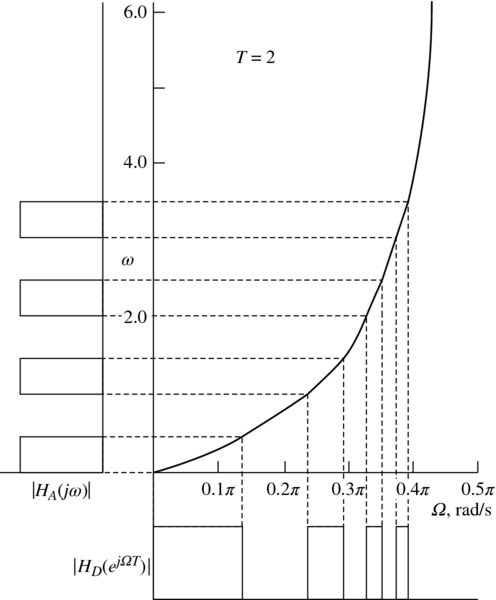
Figure 2.13 IIR filter distortion
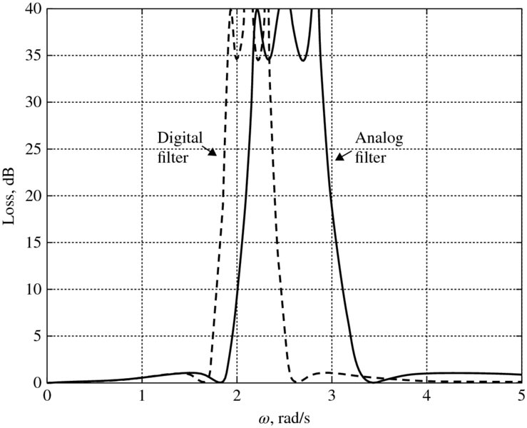
Figure 2.14 Frequency impact of warping
The main concern is to maintain stability by ensuring that the poles are located within the unit circle. There is a direct relationship between the location of these zeros and poles and the filter properties. For example, a pole on the unit circle with no zero to annihilate it will produce an infinite gain at a certain frequency (Meyer-Baese 2001).
Due to the feedback loops as shown in Figure 2.12, the structures are very sensitive to quantization errors, a feature which increases as the filter order grows. For this reason, filters are built from second-order IIR filters defined by
leading to the structure of Figure 2.15.
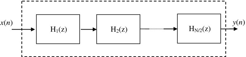
Figure 2.15 Cascade of second-order IIR filter blocks
2.4.3 Wave Digital Filters
In addition to non-recursive (FIR) and recursive (IIR) filters, a class of filter structures called WDFs is also of considerable interest as they possess a low sensitivity to coefficient variations. This is important in IIR filters as it determines the level of accuracy to which the filter coefficients have to be realized and has a direct correspondence to the dynamic range needed in the filter structure; this affects the internal wordlength sizes and filter performance which will invariably affect throughput rate.
WDFs possess a low sensitivity to attenuation due to their inherent structure, thereby reducing the loss response due to changes in coefficient representation. This is important for many DSP applications for a number of reasons: it allows short coefficient representations to be used which meet the filter specification and which involve only a small hardware cost; structures with low coefficient sensitivities also generate small round-off errors, i.e. errors that result as an effect of limited arithmetic precision within the structure. (Truncation and wordlength errors are discussed in Chapter 3.) As with IIR filters, the starting principle is to generate low-sensitivity digital filters by capturing the low-sensitivity properties of the analogue filter structures.
WDFs represent a class of filters that are modeled on classical analogue filter networks (Fettweis et al. 1986; Fettweis and Nossek 1982; Wanhammar 1999) which are typically networks configured in the lattice or ladder structure. For circuits that operate on low frequencies where the circuit dimensions are small relative to the wavelength, the designer can treat the circuit as an interconnection of lumped passive or active components with unique voltages and currents defined at any point in the circuit, on the basis that the phase change between aspects of the circuit will be negligible.
This allows a number of circuit-level design optimization techniques such as Kirchhoff’s law to be applied. However, for higher-frequency circuits, these assumptions no longer apply and the user is faced with solving Maxwell’s equations. To avoid this, the designer can exploit the fact that she is solving the problems only in certain places such as the voltage and current levels at the terminals (Pozar 2005). By exploiting specific types of circuits such as transmission lines which have common electrical propagation times, circuits can then be treated as transmission lines and modeled as distributed components characterized by their length, propagation constant and characteristic impedance.
The process of producing a WDF has been covered by Fettweis et al. (1986). The main design technique is to generate filters using transmission line filters and relate these to classical filter structures with lumped circuit elements; this allows the designer to exploit the well-known properties of these structures, termed a reference filter. The correspondence between the WDF and its reference filter is achieved by mapping the reference structure using a complex frequency variable, ψ, termed Richard’s variable, allowing the reference structure to be mapped effectively into the ψ domain.
The use of reference structures allows all the inherent passivity and lossless features to be transferred into the digital domain, achieving good filter performance and reducing the coefficient sensitivity, thereby allowing lower wordlengths to be achieved. Fettweis et al. (1986) give the simplest and most appropriate choice of ψ as the bilinear transform of the z-variable, given by
where ρ is the actual complex frequency. This variable has the property that the real frequencies ω correspond to real frequencies ϕ,
implying that the real frequencies in the reference domain correspond to real frequencies in the digital domain. Other properties described in Fettweis et al. (1986) ensure that the filter is causal. The basic principle used for WDF filter design is illustrated in Figure 2.16, taken from Wanhammar (1999). The lumped element filter is shown in Figure 2.16(a) where the various passive components, L2s, ![]() and L4s, map to R2ψ,
and L4s, map to R2ψ, ![]() and R4ψ respectively in the analogous filter given in Figure 2.16(b). Equation (2.23) is then used to map the equivalent transmission line circuit to give the ϕ domain filter in Figure 2.16(c).
and R4ψ respectively in the analogous filter given in Figure 2.16(b). Equation (2.23) is then used to map the equivalent transmission line circuit to give the ϕ domain filter in Figure 2.16(c).
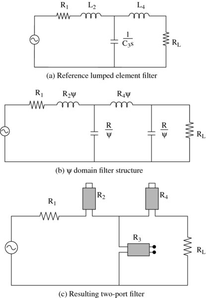
Figure 2.16 WDF configuration
WDF Building Blocks
As indicated in Figure 2.16(c), the basic WDF configuration is based upon the various one-, two- and multi-port elements. Figure 2.17 gives a basic description of the two-port element. The network can be described by incident, A, and reflected, B, waves which are related to the port currents, I1 and I2, port voltages, V1 and V2, and port resistances, R1 and R2, by (Fettweis et al. 1986)
The transfer function, S21, is given by
where
Figure 2.17 WDF building blocks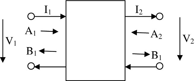
In a seminal paper, Fettweis et al. (1986) show that the loss, α, can be related to the circuit parameters, namely the inductance or capacitance and frequency, ω, such that the loss is ω = ω0, indicating that for a well-designed filter, the sensitivity of the attenuation is small through its passband, thus giving the earlier stated advantages of lower coefficient wordlengths.
As indicated in Figure 2.17, the basic building blocks for the reference filters are a number of these common two-port and three-port elements or adapters. Some of these are given in Figure 2.18, showing how they are created using multipliers and adders.
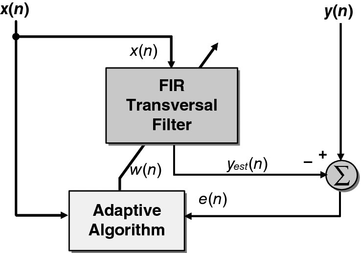
Figure 2.18 Adaptive filter system
2.5 Adaptive Filtering
The basic function of a filter is to remove unwanted signals from those of interest. Obtaining the best design usually requires a priori knowledge of certain statistical parameters (such as the mean and correlation functions) within the useful signal. With this information, an optimal filter can be designed which minimizes the unwanted signals according to some statistical criterion.
One popular measure involves the minimization of the mean square of the error signal, where the error is the difference between the desired response and the actual response of the filter. This minimization leads to a cost function with a uniquely defined optimum design for stationary inputs known as a Wiener filter (Widrow and Hoff 1960). However, it is only optimum when the statistical characteristics of the input data match the a priori information from which the filter is designed, and is therefore inadequate when the statistics of the incoming signals are unknown or changing (i.e. in a non-stationary environment).
For this situation, a time-varying filter is needed which will allow for these changes. An appropriate solution is an adaptive filter, which is inherently self-designing through the use of a recursive algorithm to calculate updates for the filter parameters. These then form the taps of the new filter, the output of which is used with new input data to form the updates for the next set of parameters. When the input signals are stationary (Haykin 2002), the algorithm will converge to the optimum solution after a number of iterations, according to the set criterion. If the signals are non-stationary then the algorithm will attempt to track the statistical changes in the input signals, the success of which depends on its inherent convergence rate versus the speed at which statistics of the input signals are changing.
In adaptive filtering, two conflicting algorithms dominate the area, the RLS and the LMS algorithm. The RLS algorithm is a powerful technique derived from the method of least squares (LS). It offers greater convergence rates than its rival LMS algorithm, but this gain is at the cost of increased computational complexity, a factor that has hindered its use in real-time applications.
A considerable body of work has been devoted to algorithms and VLSI architectures for RLS filtering with the aim of reducing this computational complexity (Cioffi 1990; Cioffi and Kailath 1984; Döhler 1991; Frantzeskakis and Liu 1994; Gentleman 1973; Gentleman and Kung 1982; Givens 1958; Götze and Schwiegelshohn 1991; Hsieh et al. 1993; McWhirter 1983; McWhirter et al. 1995; Walke 1997). Much of this work has concentrated on calculating the inverse of the correlation matrix, required to solve for the weights, in a more stable and less computationally intensive manner than straightforward matrix inversion.
The standard RLS algorithm achieves this by recursively calculating updates for the weights using the matrix inversion lemma (Haykin 2002). An alternative and very popular solution performs a set of orthogonal rotations, (e.g. Givens rotations (Givens 1958)) on the incoming data matrix, transforming it into an equivalent upper triangular matrix. The filter parameters can then be calculated by back substitution. This method, known as QR decomposition, is an extension of QR factorization that enables the matrix to be re-triangularized, when new inputs are present, without the need to perform the triangularization from scratch. From this beginning, a family of numerically stable and robust RLS algorithms has evolved from a range of QR decomposition methods such as Givens rotations (Givens 1958) and Householder transformations (Cioffi 1990).
2.5.1 Applications of Adaptive Filters
Because of their ability to operate satisfactorily in non-stationary environments, adaptive filters have become an important part of DSP in applications where the statistics of the incoming signals are unknown or changing. One such application is channel equalization (Drewes et al. 1998) where the intersymbol interference and noise within a transmission channel are removed by modeling the inverse characteristics of the contamination within the channel. Another is adaptive noise cancelation where background noise is eliminated from speech using spatial filtering. In echo cancelation, echoes caused by impedance mismatch are removed from a telephone cable by synthesizing the resounding signal and then subtracting it from the original received signal.
The key application for this research is adaptive beamforming (Litva and Lo 1996; Moonen and Proudler 1998; Ward et al. 1986). The function of a typical adaptive beamformer is to suppress signals from every direction other than the desired “look direction” by introducing deep nulls in the beam pattern in the direction of the interference. The beamformer output is a weighted combination of signals received by a set of spatially separated antennae, one primary antenna and a number of auxiliary antennae. The primary signal constitutes the input from the main antenna, which has high directivity. The auxiliary signals contain samples of interference threatening to swamp the desired signal. The filter eliminates this interference by removing any signals in common with the primary input signal.
2.5.2 Adaptive Algorithms
There is no distinct technique for determining the optimum adaptive algorithm for a specific application. The choice comes down to a balance between the range of characteristics defining the algorithms, such as rate of convergence (i.e. the rate at which the adaptive algorithm reaches within a tolerance of optimum solution); steady-state error (i.e. the proximity to an optimum solution); ability to track statistical variations in the input data; computational complexity; ability to operate with ill-conditioned input data; and sensitivity to variations in the wordlengths used in the implementation.
Two methods for deriving recursive algorithms for adaptive filters use Wiener filter theory and the LS method, resulting in the LMS and RLS algorithms, respectively. The LMS algorithm offers a very simple yet powerful approach, giving good performance under the right conditions (Haykin 2002). However, its limitations lie with its sensitivity to the condition number of the input data matrix as well as slow convergence rates. In contrast, the RLS algorithm is more elaborate, offering superior convergence rates and reduced sensitivity to ill-conditioned data. On the negative side, the RLS algorithm is substantially more computationally intensive than the LMS equivalent.
Filter coefficients may be in the form of tap weights, reflection coefficients or rotation parameters depending on the filter structure, i.e. transversal, lattice or systolic array, respectively (Haykin 2002). However, in this research both the LMS and RLS algorithms are applied to the basic structure of a transversal filter (Figure 2.18), consisting of a linear combiner which forms a weighted sum of the system inputs, x(n), and then subtracts them from the desired signal, y(n), to produce an error signal, e(n):
In Figure 2.18, w(n) and w(n + 1) are the adaptive and updated adaptive weight vectors respectively, and yest(n) is the estimation of the desired response.
2.5.3 LMS Algorithm
The LMS algorithm is a stochastic gradient algorithm, which uses a fixed step-size parameter to control the updates to the tap weights of a transversal filter as in Figure 2.18 (Widrow and Hoff 1960). The algorithm aims to minimize the mean square error, the error being the difference between y(n) and yest(n). The dependence of the mean square error on the unknown tap weights may be viewed as a multidimensional paraboloid referred to as the error surface, as depicted in Figure 2.19 for a two-tap example (Haykin 2002).
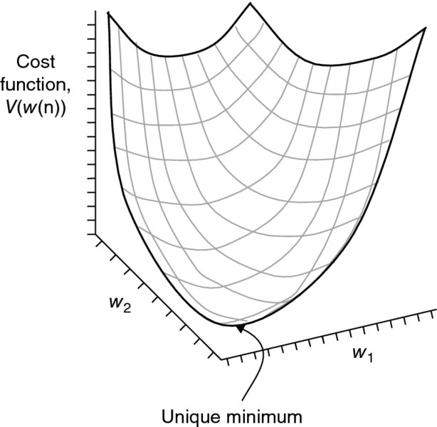
Figure 2.19 Error surface of a two-tap transversal filter
The surface has a uniquely defined minimum point defining the tap weights for the optimum Wiener solution (defined by the Wiener–Hopf equations detailed in the next subsection). However, in the non-stationary environment, this error surface is continuously changing, thus the LMS algorithm needs to be able to track the bottom of the surface.
The LMS algorithm aims to minimize a cost function, V(w(n)), at each time step n, by a suitable choice of the weight vector w(n). The strategy is to update the parameter estimate proportional to the instantaneous gradient value, ![]() , so that
, so that
where μ is a small positive step size and the minus sign ensures that the parameter estimates descend the error surface. V(w(n)) minimizes the mean square error, resulting in the following recursive parameter update equation:
The recursive relation for updating the tap weight vector (i.e. equation (2.30)) may be rewritten as
and represented as filter output
estimation error
and tap weight adaptation
The LMS algorithm requires only 2N + 1 multiplications and 2N additions per iteration for an N-tap weight vector. Therefore it has a relatively simple structure and the hardware is directly proportional to the number of weights.
2.5.4 RLS Algorithm
In contrast, RLS is a computationally complex algorithm derived from the method of least squares in which the cost function, J(n), aims to minimize the sum of squared errors, as shown in equation (2.29):
Substituting equation (2.29) into equation (2.36) gives
Converting from the discrete time domain to a matrix–vector form simplifies the representation of the equations. This is achieved by considering the data values from N samples, so that equation (2.29) becomes
which may be expressed as:
The cost function J(n) may then be represented in matrix form as
This is then multiplied out and simplified to give
where XT(n) is the transpose of X(n). To find the optimal weight vector, this expression is differentiated with respect to w(n) and solved to find the weight vector that will drive the derivative to zero. This results in a LS weight vector estimation, wLS, which is derived from the above expression and can be expressed in matrix form as
These are referred to as the Wiener–Hopf normal equations
where, ϕ(n) is the correlation matrix of the input data, X(n), and θ(n) is the cross-correlation vector of the input data, X(n), with the desired signal vector, y(n). By assuming that the number of observations is larger that the number of weights, a solution can be found since there are more equations than unknowns.
The LS solution given so far is performed on blocks of sampled data inputs. This solution can be implemented recursively, using the RLS algorithm, where the LS weights are updated with each new set of sample inputs. Continuing this adaptation through time would effectively perform the LS algorithm on an infinitely large window of data and would therefore only be suitable for a stationary system. A weighting factor may be included in the LS solution for application in non-stationary environments. This factor assigns greater importance to the more recent input data, effectively creating a moving window of data on which the LS solution is calculated. The forgetting factor, β, is included in the LS cost function (from equation (2.39)) as
where β(n − i) has the property 0 < β(n − i) ⩽ 1, i = 1, 2, …, N. One form of the forgetting factor is the exponential forgetting factor:
where λ is a positive constant with a value close to but less than one. Its value is of particular importance as it determines the length of the data window that is used and will affect the performance of the adaptive filter. The inverse of 1 − λ gives a measure of the “memory” of the algorithm. The general rule is that the longer the memory of the system, the faster the convergence and the smaller the steady-state error. However, the window length is limited by the rate of change in the statistics of the system. Applying the forgetting factor to the Wiener–Hopf normal equations (2.43)–(2.45), the correlation matrix and the cross-correlation matrix become
The recursive representations are then expressed as
or more concisely as
Likewise, θ(n) can be expressed as
Solving the Wiener–Hopf normal equations to find the LS weight vector requires the evaluation of the inverse of the correlation matrix, as highlighted by the following example matrix–vector expression below:
The presence of this matrix inversion creates an implementation hindrance in terms of both numerical stability and computational complexity. Firstly, the algorithm would be subject to numerical problems if the correlation matrix became singular. Also, calculating the inverse for each iteration involves an order of complexity N3, compared with a complexity of order N for the LMS algorithm, where N is the number of filter taps.
There are two particular methods to solve the LS solution recursively without the direct matrix inversion which reduce this complexity to order N2. The first technique, referred to as the standard RLS algorithm, recursively updates the weights using the matrix inversion lemma. The alternative and very popular solution performs a set of orthogonal rotations, e.g. Givens rotations (Givens 1958), on the incoming data transforming the square data matrix into an equivalent upper triangular matrix (Gentleman and Kung 1982). The weights can then be calculated by back substitution.
This method, known as QR decomposition (performed using one of a range of orthogonal rotation methods such as Householder transformations or Givens rotations), has been the basis for a family of numerically stable and robust RLS algorithms (Cioffi 1990; Cioffi and Kailath 1984; Döhler 1991; Hsieh et al. 1993; Liu et al. 1990, 1992; McWhirter 1983; McWhirter et al. 1995; Rader et al. 1986; Walke 1997). There are versions known as fast RLS algorithms, which manipulate the redundancy within the system to reduce the complexity to the order of N, as mentioned in Section 2.5.5.
Systolic Givens Rotations
The conventional Givens rotation QR algorithm can be mapped onto a highly parallel triangular array (referred to as the QR array (Gentleman and Kung 1982; McWhirter 1983)) built up from two types of cells, a boundary cell (BC) and an internal cell (IC). The systolic array for the conventional Givens RLS algorithm is shown in Figure 2.20. Note that the original version (Gentleman and Kung 1982) did not include the product of cosines formed down the diagonal line of BCs. This modification (McWhirter 1983) is significant as it allows the QR array to both perform the functions for calculating the weights and operate as the filter itself. That is, the error residual (a posteriori error) may be found without the need for weight vector extraction. This offers an attractive solution in applications, such as adaptive beamforming, where the output of interest is the error residual.
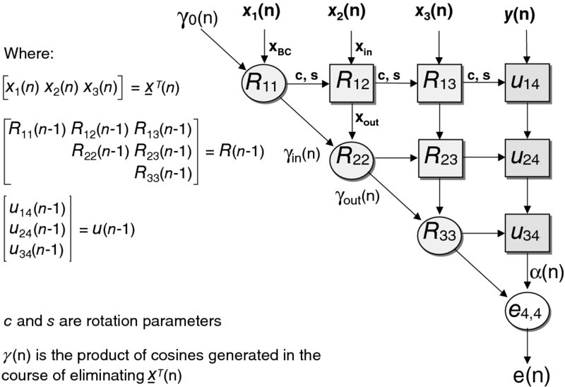
Figure 2.20 Systolic QR array for the RLS algorithm
All the cells are locally interconnected, which is beneficial, as it is interconnection lengths that have the most influence over the critical paths and power consumption of a circuit. This highly regular structure is referred to as a systolic array. Its processing power comes from the concurrent use of many simple cells rather than the sequential use of a few very powerful cells and is described in detail in the next chapter. The definitions for the BCs and ICs are depicted in Figures 2.21 and 2.22 respectively.
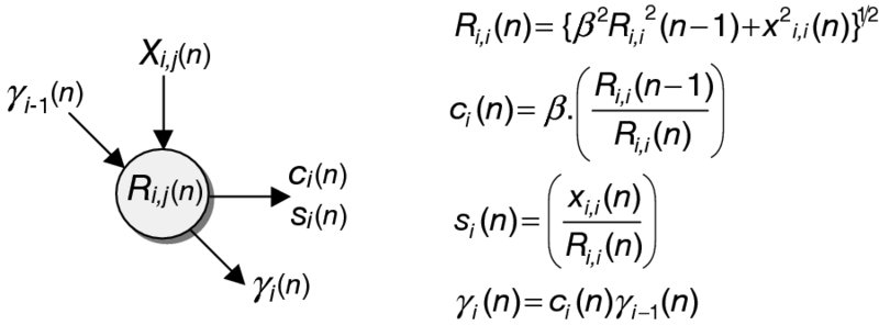
Figure 2.21 BC for QR-RLS algorithm
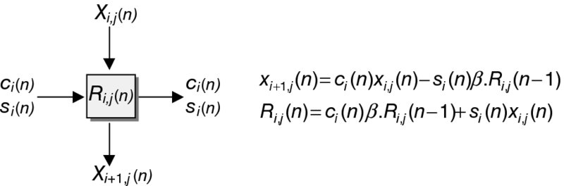
Figure 2.22 IC for QR-RLS algorithm
The data vector ![]() is input from the top of the array and is progressively eliminated by rotating it within each row of the stored triangular matrix R(n − 1) in turn. The rotation parameters c and s are calculated within a BC such that they eliminate the input, xi, i(n). These parameters are then passed unchanged along the row of ICs continuing the rotation. The output values of the ICs, xi + 1, j(n), become the input values for the next row. Meanwhile, new inputs are fed into the top of the array, and so the process repeats. In the process, the R(n) and u(n) values are updated to account for the rotation and then stored within the array to be used on the next cycle.
is input from the top of the array and is progressively eliminated by rotating it within each row of the stored triangular matrix R(n − 1) in turn. The rotation parameters c and s are calculated within a BC such that they eliminate the input, xi, i(n). These parameters are then passed unchanged along the row of ICs continuing the rotation. The output values of the ICs, xi + 1, j(n), become the input values for the next row. Meanwhile, new inputs are fed into the top of the array, and so the process repeats. In the process, the R(n) and u(n) values are updated to account for the rotation and then stored within the array to be used on the next cycle.
For the RLS algorithm, the implementation of the forgetting factor, λ, and the product of cosines, γ, need to be included within the equations. Therefore the operations of the BCs and ICs have been modified accordingly. A notation has been assigned to the variables within the array. Each R and u term has a subscript, denoted by (i, j), which represents the location of the elements within the R matrix and u vector. A similar notation is assigned to the X input and output variables. The cell descriptions for the updated BCs and ICs are shown in Figures 2.21 and 2.22, respectively. The subscripts are coordinates relating to the position of the cell within the QR array.
2.5.5 Squared Givens Rotations
There are division and square root operations within the cell computation for the standard Givens rotations (Figures 2.21 and 2.22). There has an extensive body of research into deriving Givens rotation QR algorithms which avoid these complex operations, while reducing the overall number of computations (Cioffi and Kailath 1984; Döhler 1991; Hsieh et al. 1993; Walke 1997). One possible QR algorithm is the squared Givens rotation (SGR) (Döhler 1991). Here the Givens algorithm has been manipulated to remove the need for the square root operation within the BC and half the number of multipliers in the ICs.
Studies by Walke (1997) showed that this algorithm provided excellent performance within adaptive beamforming at reasonable wordlengths (even with mantissa wordlengths as short as 12 bits with an increase of 4 bits within the recursive loops). This algorithm turns out to be a suitable choice for the adaptive beamforming design. Figure 2.23 depicts the SFG for the SGR algorithm, and includes the BC and IC descriptions.
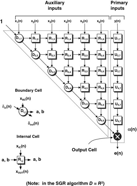
Figure 2.23 Squared Givens Rotations QR-RLS algorithm
This algorithm still requires the dynamic range of floating-point arithmetic but offers reduced size over fixed-point algorithms, due to the reduced wordlength and operations requirement. It has the added advantage of allowing the use of a multiply-accumulate operation to update R. At little cost in hardware, the wordlength of the accumulator can be increased to improve the accuracy to which R is accumulated, while allowing the overall wordlength to be reduced. This has been referred to as the Enhanced SGR algorithm (E-SGR) (Walke 1997).
However, even with the level of computation reduction achievable by the SGR algorithm, the complexity of the QR cells is still large. In addition, the number of processors within the QR array increases quadratically with the number of inputs, such that for an N-input system, (N2 + N)/2 QR processors are required; furthermore, implementing a processor for each cell could offer data rates far greater than those required by most applications. The following section details the process of deriving an efficient architecture with generic properties for implementing the SGR QR-RLS algorithm.
2.6 Final Comments
The chapter has given a brief review of DSP algorithms with the aim of providing a foundation for the work presented in this book. Some of the examples have been the focus of direct implementation using FPGA technology with the aim of giving enhanced performance in terms of the samples produced per second or a reduction in power consumption. The main focus has been to provide enough background to understand the examples, rather than an exhaustive primer for DSP.
In particular, the material has concentrated on the design of FIR and IIR filtering as this is a topic for speed optimization, particularly the material in Chapter 8, and the design of RLS filters, which is the main topic of Chapter 11 and considers the development of an IP core for an RLS filter solved by QR decomposition. These chapters represent a core aspect of the material in this book.
Bibliography
- Bourke P 1999 Fourier method of designing digital filters. Available at http://paulbourke.net/miscellaneous/filter/ (accessed April 2, 2016).
- Cioffi J 1990 The fast Householder filters RLS adaptive algorithm RLS adaptive filter. In Proc. IEEE Int. Conf. on Acoustics, Speech and Signal Processing, pp. 1619–1621.
- Cioffi J, Kailath T 1984 Fast, recursive-least-squares transversal filters for adaptive filtering. IEEE Trans. on ASSP, 32(2), 304–337.
- Cooley JW, Tukey JW 1965 An algorithm for the machine computation of the complex Fourier series. Mathematics of Computation, 19, 297–301.
- Daubechies I 1992 Ten Lectures on Wavelets. Society for Industrial and Applied Mathematics, Philadelphia.
- Döhler R 1991 Squared Givens rotation. IMA Journal of Numerical Analysis, 11(1), 1–5.
- Drewes C, Hasholzner R, Hammerschmidt JS 1998 On implementation of adaptive equalizers for wireless ATM with an extended QR-decomposition-based RLS-algorithm. In Proc. IEEE Intl Conf. on Acoustics, Speech and Signal Processing, pp. 3445–3448.
- Fettweis A, Gazsi L, Meerkotter K 1986 Wave digital filter: Theory and practice. Proc. IEEE, 74(2), pp. 270–329.
- Fettweis A, Nossek J 1982 On adaptors for wave digital filter. IEEE Trans. on Circuits and Systems, 29(12), 797–806.
- Frantzeskakis EN, Liu KJR 1994 A class of square root and division free algorithms and architectures for QRD-based adaptive signal processing. IEEE Trans. on Signal Proc. 42(9), 2455–2469.
- Gentleman WM 1973 Least-squares computations by Givens transformations without square roots, J. Inst. Math. Appl., 12, 329–369.
- Gentleman W, Kung H 1982 Matrix triangularization by systolic arrays. In Proc. SPIE, 298, 19–26.
- Givens W 1958 Computation of plane unitary rotations transforming a general matrix to triangular form. J. Soc. Ind. Appl. Math, 6, 26–50.
- Götze J, Schwiegelshohn U 1991 A square root and division free Givens rotation for solving least squares problems on systolic arrays. SIAM J. Sci. Stat. Compt., 12(4), 800–807.
- Haykin S 2002 Adaptive Filter Theory. Publishing House of Electronics Industry, Beijing.
- Hsieh S, Liu K, Yao K 1993 A unified approach for QRD-based recursive least-squares estimation without square roots. IEEE Trans. on Signal Processing, 41(3), 1405–1409.
- Litva J, Lo TKY 1996 Digital Beamforming in Wireless Communications, Artec House, Norwood, MA.
- Liu KJR, Hsieh S, Yao K 1990 Recursive LS filtering using block Householder transformations. In Proc. of Int. Conf. on Acoustics, Speech and Signal Processing, pp. 1631–1634.
- Liu KJR, Hsieh S, Yao K 1992 Systolic block Householder transformations for RLS algorithm with two-level pipelined implementation. IEEE Trans. on Signal Processing, 40(4), 946–958.
- Lynn P, Fuerst W 1994 Introductory Digital Signal Processing with Computer Applications. John Wiley & Sons, Chicester.
- Mallat SG 1989 A theory for multiresolution signal decomposition: the wavelet representation. IEEE Trans. on Pattern Analysis and Machine Intelligence, 11(7), 674–693.
- McWhirter J 1983 Recursive least-squares minimization using a systolic array. In Proc. SPIE, 431, 105–109.
- McWhirter JG, Walke RL, Kadlec J 1995 Normalised Givens rotations for recursive least squares processing. In VLSI Signal Processing, VIII, pp. 323–332.
- Meyer-Baese U 2001 Digital Signal Processing with Field Programmable Gate Arrays, Springer, Berlin.
- Moonen M, Proudler IK 1998 MDVR beamforming with inverse updating. In Proc. European Signal Processing Conference, pp. 193–196.
- Nyquist H 1928 Certain topics in telegraph transmission theory. Trans. American Institute of Electrical Engineers, 47, 617–644.
- Pozar DM 2005 Microwave Engineering. John Wiley & Sons, Hoboken, NJ.
- Rabiner L, Gold B 1975 Theory and Application of Digital Signal Processing. Prentice Hall, New York.
- Rader CM, Steinhardt AO 1986 Hyperbolic Householder transformations, definition and applications. In Proc. of Int. Conf. on Acoustics, Speech and Signal Processing, pp 2511–2514.
- Shannon CE 1949 Communication in the presence of noise. Proc. Institute of Radio Engineers, 37(1), 10–21.
- Walke R 1997 High sample rate Givens rotations for recursive least squares. PhD thesis, University of Warwick.
- Wanhammar L 1999 DSP Integrated Circuits Academic Press, San Diego, CA.
- Ward CR, Hargrave PJ, McWhirter JG 1986 A novel algorithm and architecture for adaptive digital beamforming. IEEE Trans. on Antennas and Propagation, 34(3), 338–346.
- Widrow B, Hoff, Jr. ME 1960 Adaptive switching circuits. IRE WESCON Conv. Rec., 4, 96–104.
- Williams C 1986 Designing Digital Filters. Prentice Hall, New York.