Chapter 13
Fiber-Optic System Advantages
The following ETA Fiber-Optics Installer competencies are covered in this chapter:
 Compare the bandwidth advantages of optical fiber over twisted pair and coaxial copper cables.
- Compare the attenuation advantages of optical fiber over twisted pair and coaxial copper cables.
- Explain the electromagnetic immunity advantages of fiber-optic cable over copper cable.
- Describe the size advantages of fiber-optic cable over copper cable.
- Describe the weight-saving advantages of fiber-optic cable over copper cable.
- Describe the security advantages of fiber-optic cable over copper cable.
- Compare the safety advantages of fiber-optic cables over copper cables.
Up to this point, you have learned about transmitters, receivers, connectors, splices, and fiber-optic cable. These pieces are some of the building blocks of a fiber-optic system. A basic fiber-optic system contains a transmitter, receiver, fiber-optic cable, and connectors.
This chapter explores the performance advantages that optical fiber has over twisted pair and coaxial copper cable.
In this chapter, you will learn to
- Calculate the bandwidth for a length of optical fiber
- Calculate the attenuation for a length of optical fiber
The Advantages of Optical Fiber over Copper
In this chapter, we will examine seven fiber-optic system performance areas and compare the performance of optical fiber to twisted pair and coaxial copper cable. Performance in this comparison will be evaluated in the areas of bandwidth, attenuation, electromagnetic immunity, size, weight, safety, and security. The fiber-optic system will operate at an 850nm wavelength with a VCSEL source.
Performance data for the laser-optimized optical fiber will be taken from the ANSI/TIA-568-C.3 and ISO/IEC 11801 standards. It will be compared to both Category 6A twisted pair cable and RG6 coaxial cable. Performance data for the Category 6A cable will be taken from the ANSI/TIA-568-C.2 Commercial Building Telecommunication Cabling Standard Part 2: Balanced Twisted-Pair Cabling Components, and the performance data for the RG6 coaxial cable is derived by averaging the values found in several manufacturers' datasheets.
All the comparisons in this chapter are based on latest standards and datasheets that were available as of this writing.
Bandwidth
Bandwidth is a popular buzzword these days. We are bombarded with commercials advertising high-speed downloads from a cable modem, satellite, or fiber-to-the-home (FTTH). The competition to sell us bandwidth is fierce. As you learned in Chapter 1, “History of Fiber Optics and Broadband Access,” while the basic broadband speed was defined with a 3Mbps download speed, more than 94 percent of the homes in America exceed 10Mbps. More than 75 percent have download speeds greater than 50Mbps, 47 percent have download speeds greater than 100Mbps, and more than 3 percent enjoy download speeds greater than one billion bits (a gigabit) per second (Gbps).
In earlier chapters, we looked at the physical properties of the optical fiber and fiber-optic light source that limit bandwidth. You learned that single-mode systems with laser transmitters offer the greatest bandwidth over distance and that multimode systems with LED transmitters offer the least bandwidth and are limited in transmission distance. You also learned that the bandwidth of the optical fiber is inversely proportional to its length. In other words, as the length of the optical fiber increases, the bandwidth of the optical fiber decreases.
So how does length affect the bandwidth of a copper cable? Well, when it comes to cable length, copper suffers just as optical fiber does. When the length of a copper cable is increased, the bandwidth for that cable decreases. So if both copper and optical fiber lose bandwidth over distance, why is optical fiber superior to copper? To explain that, we will look at the minimum bandwidth requirements defined in ANSI/TIA-568-C.3 and ISO/IEC 11801 for multimode optical fiber, ANSI/TIA-568-C.2 for unshielded twisted pair (UTP) Category 6A cable, and the datasheets for RG6 coaxial cable.
Remember that the values defined in ANSI/TIA-568-C.2, ANSI/TIA-568-C.3, and ISO/IEC 11801 are the minimum values that a manufacturer needs to achieve. There are many manufacturers offering optical fiber and copper cables that exceed these minimum requirements. However, for this comparison, only values defined in these two standards will be used.
One of the problems in doing this comparison is cable length. ANSI/TIA-568-C.2 defines Category 6A performance at a maximum physical length of 100m at frequencies up to 500MHz. ANSI/TIA-568-C.3 and ISO/IEC 11801 do not define a maximum bandwidth at a maximum optical fiber length. As you learned in Chapter 5, “Optical Fiber Characteristics,” ANSI/TIA-568-C.3 and ISO/IEC 11801 define multimode optical fiber bandwidth two ways depending on the type of light source. In this comparison the 850nm VCSEL is used with 50/125μm laser-optimized optical fiber (OM4, Type A1a.3, TIA 492AAAD). The minimum effective modal bandwidth-length product in MHz · km is 4700 for this combination, as shown in Table 13.1.
Table 13.1 Characteristics of ANSI/TIA-568-C.3 and ISO/IEC 11801-recognized optical fibers
| Optical fiber cable type | Wavelength (nm) | Maximum attenuation (dB/km) | Minimum overfilled modal bandwidth-length product (MHz · km) | Minimum effective modal bandwidth-length product (MHz · km) |
| 62.5/125μm Multimode OM1 Type A1b TIA 492AAAA |
850 1300 |
3.5 1.5 |
200 500 |
Not Required Not Required |
| 50/125μm Multimode OM2 TIA 492AAAB Type A1a.1 |
850 1300 |
3.5 1.5 |
500 500 |
Not Required Not Required |
| 850nm laser-optimized 50/125μm Multimode OM3 Type A1a.2 TIA 492AAAC |
850 1300 |
3.5 1.5 |
1500 500 |
2000 Not Required |
| 850nm laser-optimized 50/125μm Multimode OM4 Type A1a.3 TIA 492AAAD |
850 1300 |
3.5 1.5 |
3500 500 |
4700 Not Required |
| Single-mode Indoor-outdoor OS1 Type B1.1 TIA 492CAAA OS2 Type B1.3 TIA 492CAAB |
1310 1550 |
0.5 0.5 |
N/A N/A |
N/A N/A |
| Single-mode Inside plant OS1 Type B1.1 TIA 492CAAA OS2 Type B1.3 TIA 492CAAB |
1310 1550 |
1.0 1.0 |
N/A N/A |
N/A N/A |
| Single-mode Outside plant OS1 Type B1.1 TIA 492CAAA OS2 Type B1.3 TIA 492CAAB |
1310 1550 |
0.5 0.5 |
N/A N/A |
N/A N/A |
To do this comparison, we will need to calculate the bandwidth limitations for 100m of OM4 laser-optimized multimode optical fiber, as shown here:
The 100m OM4 laser-optimized multimode optical fiber has a bandwidth 94 times greater than the Category 6A cable. This clearly shows that optical fiber offers incredible bandwidth advantages over Category 6A cable.
Now that we have seen how the bandwidth of OM4 laser-optimized multimode optical fiber with an 850nm VCSEL source greatly exceeds that of Category 6A cable, let's do a comparison with RG6 coaxial cable. This cable has been chosen because it is widely used in homes and buildings for video distribution. Remember the performance data for the RG6 coaxial cable is taken from the average of several manufacturers' datasheets. ANSI/TIA-568-C does not define performance parameters for RG6 coaxial cable.
An RG6 coaxial cable with a transmission frequency of 4GHz has roughly the same 100m transmission distance characteristics as a Category 6A cable at 500MHz. We know from the previous comparison that a 100m length of 50/125μm multimode optical fiber will support transmission frequencies up to 47GHz over that same distance with an 850nm light source. In this comparison, the laser-optimized multimode optical fiber offers a bandwidth advantage 11.75 times greater than the RG6 coaxial cable.
These comparisons have demonstrated the bandwidth advantages of optical fiber over copper cable. The comparisons were done at very short distances because at this point we have not addressed how attenuation in a copper cable changes with the transmission frequency, whereas in an optical fiber, attenuation is constant regardless of the transmission frequency.
Attenuation
All transmission mediums lose signal strength over distance. As you know, this loss of signal strength is called attenuation and is typically measured in decibels. Optical fiber systems measure attenuation using optical power. Copper cable systems typically use voltage drop across a defined load at various transmission frequencies to measure attenuation. The key difference here is not that optical fiber uses power and copper uses voltage. The key difference is that attenuation in copper cables is measured at different transmission frequencies. This is not the case with optical fiber, where attenuation is measured with a continuous wave light source.
The attenuation in a copper cable increases as the transmission frequency increases. Table 13.2 shows the maximum worst pair insertion loss for a 100m horizontal Category 5e and Category 6A cable as defined in ANSI/TIA-568-C.2. This table clearly shows the effects that transmission frequency has on a copper cable.
Table 13.2 Horizontal cable insertion loss, worst pair*
| Frequency (MHz) | Category 5e (dB) | Category 6A (dB) |
| 1.0 | 2.0 | 2.1 |
| 4.0 | 4.1 | 3.8 |
| 8.0 | 5.8 | 5.3 |
| 10.0 | 96.5 | 5.9 |
| 16.0 | 8.2 | 7.5 |
| 20.0 | 9.3 | 8.4 |
| 25.0 | 10.4 | 9.4 |
| 31.25 | 11.7 | 10.5 |
| 62.5 | 17.0 | 15.0 |
| 100.0 | 22.0 | 19.1 |
| 200.0 | 27.6 | |
| 300.0 | 34.3 | |
| 400.0 | 40.1 | |
| 500.0 | 45.3 |
* For a length of 100m (328')
The maximum allowable attenuation in an optical fiber is defined in ANSI/TIA-568-C.3 and ISO/IEC 11801. Table 13.3 shows the attenuation portion of the optical fiber cable transmission performance parameters. This table defines attenuation for both multimode and single-mode optical fibers. You will notice that there is no column for transmission frequency in this table. That is because optical fiber does not attenuate as the transmission frequency increases like copper cable does.
Table 13.3 ANSI/TIA-568-C.3 and ISO/IEC 11801 optical fiber cable attenuation performance parameters
| Optical fiber cable type | Wavelength (nm) | Maximum attenuation (dB/km) |
| 50/125μm multimode | 850 1300 |
3.5 1.5 |
| 62.5/125μm multimode | 850 1300 |
3.5 1.5 |
| Single-mode inside plant cable | 1310 1550 |
1.0 1.0 |
| Single-mode outside plant cable | 1310 1550 |
0.5 0.5 |
Now that you know how optical fiber and copper cable attenuate, let's do a comparison. The first comparison will put optical fiber up against Category 6A cable. The distance will be 100m and the transmission frequency will be 500MHz.
Table 13.2 lists 45.3dB for the worst-case attenuation for the Category 6A cable at 500MHz. This means the Category 6A cable loses 99.997 percent of its energy over a distance of 100m at that transmission frequency. As you learned in Chapter 5, the attenuation of an optical fiber is different for each wavelength. Table 13.3 lists the maximum attenuation in dB/km. We can solve for the maximum attenuation at both wavelengths as shown here.
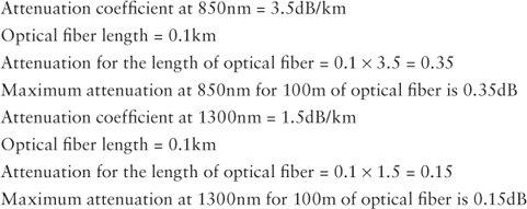
The equations show that multimode optical fiber loses 7.7 percent of the light energy from the transmitter over the 100m distance at 850nm. At 1300nm, the loss is only 3.4 percent. However, the Category 6A cable loses 99.997 percent of the transmitted signal over that distance. This means that the Category 6A cable loses roughly 31261 times more energy than the optical fiber 850nm and roughly 32734 times more energy at 1300nm.
This comparison clearly shows the attenuation advantages of optical fiber over Category 6A cable.
Now let's compare the same optical fiber at the same wavelengths to an RG6 coaxial cable. For this comparison, the RG6 attenuation characteristics are taken from the average of several different manufacturers' published datasheets, as shown in Table 13.4.
Table 13.4 RG6 cable insertion loss*
| Frequency (MHz) | RG6 (dB) |
| 1.0 | 0.8 |
| 5.0 | 1.7 |
| 100 | 6.4 |
| 200 | 9.5 |
| 500 | 14.0 |
| 1,000 | 21.3 |
| 3,000 | 38.8 |
| 4,500 | 49.0 |
* For a length of 100m (328')
As you look at Table 13.4, you can see that RG6 coaxial cable easily outperforms Category 5e and 6A cable. However, it does not even begin to approach the multimode optical fiber operating at 850nm or 1300nm. The RG6 coaxial cable has 14dB of attenuation at a transmission frequency of 500MHz over a distance of 100m. Whereas the Category 6A cable lost 99.997 percent of its signal strength, in the previous comparison the RG6 coaxial cable lost only 96 percent of its energy over the same distance.
These comparisons should make it clear that optical fiber has an enormous attenuation advantage over copper cable. The comparisons were done only with multimode optical fiber. Outside-plant, single-mode optical fiber greatly outperforms multimode optical fiber. Single-mode optical fiber links are capable of transmission distances greater than 80km without re-amplification. Based on the previous comparisons, Category 6A cable would require re-amplification every 100m at a transmission frequency of 500MHz. The RG6 coaxial cable would require re-amplification every 325m at a transmission frequency of 500MHz.
An 80km RG6 coaxial cable link transmitting a frequency of 500 MHz would require roughly 246 amplifiers to re-amplify the signal. However, the single-mode optical fiber link would not require re-amplification. Optical fiber links are unsurpassed in transmission distance.
Electromagnetic Immunity
Electromagnetic interference (EMI) is electromagnetic energy, sometimes referred to as noise, which causes undesirable responses, degradation, or complete system failure. Systems using copper cable are vulnerable to the effects of EMI because a changing electromagnetic field will induce current flow in a copper conductor. Optical fiber is a dielectric or an insulator, and current does not flow through insulators. What this means is that EMI has no effect on the operation of an optical fiber.
Let's take a look at some examples of EMI-induced problems in a copper system. A Category 6A cable has four pairs of twisted conductors. The conductors are twisted to keep the impedance uniform along the length of the cable and to decrease the effects of EMI by canceling out opposing fields. Two of the conductor pairs may be used to transmit and two of the conductor pairs may be used to receive.
For this example, only one pair is transmitting and one pair is receiving. The other two pairs in the cable are not used. Think of each pair of conductors as an antenna. The transmitting pair is the broadcasting antenna and the receiving pair is picking up that transmission just like your car radio antenna.
The data on the transmitting pair is broadcast and picked up by the receiving pair. This is called crosstalk. If enough current is induced into the receiving pair, the operation of the system can be affected. This is one reason why it is so critical to maintain the twists in a Category 6A cable.
Would we have this problem with an optical fiber? Does crosstalk exist in optical fiber? Regardless of the number of transmitting and receiving optical fibers in a cable assembly, crosstalk does not occur. To have crosstalk in an optical fiber cable assembly, light would have to leave one optical fiber and enter one of the other optical fibers in the cable assembly. Because of total internal reflection, under normal operating conditions light never leaves the optical fiber. Therefore, crosstalk does not exist in optical fiber cable assemblies.
Now let's take a look at another EMI scenario. Copper cables are being routed through a manufacturing plant. This manufacturing plant houses large-scale electromechanical equipment that generates a considerable amount of EMI, which creates an EMI-rich environment.
Routing cables through an EMI-rich environment can be difficult. Placing the cables too close to the EMI-generating source can induce unwanted electrical signals strong enough to cause systems to function poorly or stop operating altogether. Copper cables used in EMI-rich environments typically require electrical shielding to help reduce the unwanted electrical signals. In addition to the electrical shielding, the installer must be aware of the EMI-generating sources and ensure that the copper cables are routed as far as possible from these sources.
Routing copper cables through an EMI-rich environment can be challenging, time-consuming, and expensive. However, optical fiber cables can be routed through an EMI-rich environment with no impact on system performance. The fiber-optic installer is free to route the optical fiber as efficiently as possible. Optical fiber is very attractive to every industry because it is immune to EMI.
Size and Weight
You must take into account the size of any cable when preparing for an installation. Often fiber-optic cables will be run through existing conduits or raceways that are partially or almost completely filled with copper cable. This is another area where small fiber-optic cable has an advantage over copper cable.
Let's do a comparison and try to determine the reduced-size advantage that fiber-optic cable has over copper cable. A common size for a coated optical fiber is typically 250μm in diameter. You learned that ribbon fiber-optic cables sandwich up to 12-coated optical fibers between two layers of Mylar tape. Eighteen of these ribbons stacked on top of each other form a rectangle roughly 4.5mm by 3mm. This rectangle can be placed inside a buffer and surrounded by a strength member and jacket to form a cable. The overall diameter of this cable would be 16.5mm (0.65″), only slightly larger than a bundle of four RG6 coaxial cables or a bundle of four Category 6A cables.
So how large would a copper cable have to be to offer the same performance as the 216 optical fiber ribbon cable? That would depend on transmission distance and the optical fiber data rate. Because we have already discussed Category 6A performance, let's place a bundle of Category 6A cables up against the 216 optical fiber ribbon cable operating at a modest 2.5Gbps data rate over a distance of just 100m.
A Category 6A cable contains four conductor pairs and each pair is capable of a 500MHz transmission over 100m. As you learned earlier in this chapter, a 500MHz transmission carries 1 billion symbols per second. If each symbol is a bit, the 500MHz Category 6A cable is capable of a 1Gbps transmission rate. When the performance of each pair is combined, a single Category 6A cable is capable of a 4Gbps transmission rate over a distance of 100m.
Now let's see how many Category 6A cables will be required to provide the same performance as the 216 optical fiber ribbon cable. The 216 optical fiber ribbon cable has a combined data transmission rate of 540Gbps (2.5Gbps × 216). When we divide 540Gbps by 4Gbps, we see that 135 Category 6A cables are required to equal the performance of this modest fiber-optic system.
When 135 Category 6A cables are bundled together, they are roughly 3.4″ in diameter. As noted earlier in this chapter, the 216 optical fiber ribbon cable is approximately the size of four Category 6A cables bundled together. The Category 6A bundle thus has a volume roughly 27.4 times greater than the 216 optical fiber ribbon cable. In other words, Category 6A bundles need 27.4 times more space in the conduit than the 216 optical fiber ribbon cable.
The comparison we just performed is very conservative. The distance we used was kept very short and the transmission rate for the optical fiber was kept low. We can get even a better appreciation for the cable size reduction fiber-optic cable offers if we increase the transmission distance and the data rate.
In this comparison, let's increase the transmission distance to 1000m and the data transmission rate to 10Gbps. The bandwidth of a copper cable decreases as distance increases, just as with fiber-optic cables. Because we have increased the transmission distance by a factor of 10, it's fair to say that the Category 6A cable bandwidth will decrease by a factor of 10 over 1000m.
With a reduction in bandwidth by a factor of 10, we will need ten times more Category 6A cables to equal the old 2.5Gbps performance. In other words, we need 1350 Category 6A cables bundled together. In this comparison, however, the bandwidth has been increased from 2.5Gbps to 10Gbps. This means we have to quadruple the number of Category 6A cables to meet the bandwidth requirement. We now need 5400 Category 6A cables bundled together. Imagine how many cables we would need if the transmission distance increased to 80,000m. We would need a whopping 432,000 Category 6A cables bundled together.
These comparisons vividly illustrate the size advantage that fiber-optic cables have over copper cables. The advantage becomes even more apparent as distances increase. The enormous capacity of such a small cable is exactly what is needed to install high-bandwidth systems in buildings where the conduits and raceways are almost fully populated with copper cables.
Now that we have calculated the size advantages of optical fiber over Category 6A cable, let's look at the weight advantages. It is pretty easy to see that thousands or tens of thousands of Category 6A cables bundled together will outweigh a ribbon fiber-optic cable 0.65″ in diameter. It's difficult to state exactly how much less a fiber-optic cable would weigh than a copper cable performing the same job—there are just too many variables in transmission distance and data rate. However, it's not difficult to imagine the weight savings that fiber-optic cables offer over copper cables. These weight savings are being employed in commercial aircraft, military aircraft, and the automotive industries, just to mention a few.
Security
We know that optical fiber is a dielectric and because of that it is immune to EMI. So why is an optical fiber secure and virtually impossible to tap? Because of total internal reflection, optical fiber does not radiate.
In Chapter 5, you learned about macrobends. Excessive bending on an optical fiber will cause some of the light energy to escape the core and cladding. This light might penetrate the coating, buffer, strength member, and jacket. This energy is detectable by means of a fiber identifier.
Fiber identifiers detect light traveling through an optical fiber by inserting a macrobend. Photodiodes are placed against the jacket or buffer of the fiber-optic cable on opposite sides of the macrobend. The photodiodes detect the light that escapes from the fiber-optic cable. The light energy detected by the photodiodes is analyzed by the electronics in the fiber identifier. The fiber identifier can typically determine the presence and direction of travel of the light.
If the fiber identifier can insert a simple macrobend and detect the presence and direction of light, why is fiber secure? Detecting the presence of light and determining the source of the light does not require much optical energy. However, as you learned earlier in this chapter, a fiber-optic receiver typically has a relatively small window of operation. In other words, the fiber-optic receiver typically needs at least 10 percent of the energy from the transmitter to accurately decode the signal on the optical fiber. Inserting a macrobend in a fiber-optic cable and directing 10 percent of the light energy into a receiver is virtually impossible. A macrobend this severe would also be very easy to detect with an optical time-domain reflectometer (OTDR). There is no transmission medium more secure than optical fiber.
Safety
Electrical safety is always a concern when working with copper cables. Electrical current flowing through copper cable poses shock, spark, and fire hazards. Optical fiber is a dielectric that cannot carry electrical current; therefore, it presents no shock, spark, or fire hazard.
Because optical fiber is a dielectric, it also provides electrical isolation between electrical equipment. Electrical isolation eliminates ground loops, eliminates the potential shock hazard when two pieces of equipment at different potentials are connected together, and eliminates the shock hazard when one piece of equipment is connected to another with a ground fault.
Ground loops are typically not a safety problem; they are usually an equipment operational problem. They create unwanted noise that can interfere with equipment operation. A common example of a ground loop is the hum or buzz you hear when an electric guitar is plugged into an amplifier with a defective copper cable or electrical connection. Connecting two pieces of equipment together with optical fiber removes any path for current flow, which eliminates the ground loop.
Using copper cable to connect two pieces of equipment that are at different electrical potentials poses a shock hazard. It's not uncommon for two grounded pieces of electrical equipment separated by distance to be at different electrical potentials. Connecting these same two pieces of equipment together with optical fiber poses no electrical shock hazard.
If two pieces of electrical equipment are connected together with copper cable and one develops a ground fault, there is now a potential shock hazard at both pieces of equipment. Everyone is likely to experience, or hear of someone experiencing, a ground fault at least once in their life. A common example is when you touch an appliance such as an electric range or washing machine and experience a substantial electrical shock. If the piece of equipment that shocked you was connected to another piece of equipment with a copper cable, there is a possibility that someone touching the other piece of equipment would also be shocked. If the two pieces of equipment were connected with optical fiber, the shock hazard would exist only at the faulty piece of equipment.
Nonconductive fiber-optic cables offer some other advantages, too. They do not attract lightning any more than any other dielectric. They can be run through areas where faulty copper cables could pose a fire or explosion hazard. The only safety requirement that Article 770 of the NEC places on nonconductive fiber-optic cables addresses the type of jacket material. When electrical safety, spark, or explosion hazards are a concern, there is no better solution than optical fiber.
Summary
This chapter explained the performance advantages that optical fiber has over copper cable. Optical fiber is the highest performance transmission medium available today, boasting incredible bandwidth with very little attenuation over great distances. Fiber-optic cables the size of a garden hose can hold hundreds of optical fibers each capable of carrying billions of bits of data per second. They also offer better security and safety.
Exam Essentials
- Describe the bandwidth advantages of optical fiber over twisted pair and coaxial copper cables. Remember that single-mode systems with laser transmitters offer the greatest bandwidth and that multimode systems with LED transmitters offer the least bandwidth. The bandwidth of optical fiber and copper cable is inversely proportional to its length. In other words, as the length of the optical fiber or copper cable increases, the bandwidth of the optical fiber or copper cable decreases.
- Describe the attenuation advantages of optical fiber over twisted pair and coaxial copper cables.
Remember that all transmission mediums lose signal strength over distance and the loss of signal strength, or attenuation, is typically measured in decibels. Optical fiber systems measure attenuation using optical power. Copper cable systems typically use voltage drop across a defined load at various transmission frequencies to measure attenuation.
Remember that attenuation in copper cables is measured at different frequencies. This is not the case with optical fiber, where attenuation is measured with a continuous wave light source that is not modulated. The attenuation in a copper cables increases as the transmission frequency increases. This is not the case with optical fiber, where transmission frequency has no impact on attenuation.
- Describe the electromagnetic advantages of optical fiber over copper cable. You need to know that EMI is electromagnetic energy that causes undesirable responses, degradation, or complete system failure. Systems using copper cable are vulnerable to the effects of EMI because a changing electromagnetic field will induce current flow in a copper conductor. Optical fiber is a dielectric and current does not flow through optical fiber. Thus EMI has no effect on the operation of an optical fiber, and fiber-optic cables do not suffer from crosstalk as copper cables do.
- Describe the size advantages of fiber-optic cable over copper cable. You need to know that a copper cable and fiber-optic cable with similar performance characteristics may differ greatly in size. There is no rule of thumb for size difference; however, the fiber-optic cable may be up to hundreds of times smaller than the copper cable.
- Describe the weight-saving advantages of fiber-optic cable over copper cable. You need to know that a copper cable and fiber-optic cable with similar performance characteristics may greatly differ in weight. There is no rule of thumb for weight difference; however, the fiber-optic cable may be up to hundreds of times lighter than the copper cable.
- Describe the security advantages of fiber-optic cable over copper cable. You need to know that because of total internal reflection, optical fiber does not radiate, making it virtually impossible to tap. Optical fiber is the most secure transmission medium available.
- Describe the safety advantages of fiber-optic cable over copper cable. You need to know that optical fiber is a dielectric that cannot carry electrical current and presents no shock, spark, or fire hazard. Optical fiber also provides electrical isolation between electrical equipment.
Review Questions
- Optical fiber __________ offers bandwidth and __________ attenuation than twisted pair or coaxial cable.
A. Less, more
B. Equal, more
C. Greater, more
D. Greater, less
Hint: Also known as information carrying capacity and loss
- Optical fiber is a __________. Therefore it is immune to the effects of EMI.
A. Conductor
B. Composite
C. Dielectric
D. Radiator
Hint: Resists the flow of current
- Fiber-optic cables are __________ and __________ than copper cables with comparable transmission frequency performance.
A. Larger, heavier
B. Smaller, lighter
C. Smaller, heavier
D. Larger, lighter
Hint: The difference in size and weight increases considerably as the transmission distance increases.
- Fiber-optic cables do not __________ light energy; therefore they are virtually immune to being tapped, which makes them very secure.
A. Rotate
B. Receive
C. Detect
D. Radiate
Hint: Total internal reflection
- Optical fiber does not __________ electricity and offers safety advantages over copper cables.
A. Rotate
B. Conduct
C. Detect
D. Radiate
Hint: It provides electrical isolation between electrical equipment.
Chapter Exercises
Calculate the Bandwidth for a Length of Optical Fiber
The minimum effective bandwidth-length product in MHz · km is defined in TIA-568-C.3 and ISO/IEC 11801.
Refer to the following table and determine the minimum effective modal bandwidth for 300 meters of OM4 optical fiber at a wavelength of 850nm.
| Optical fiber cable type | Wavelength (nm) | Maximum attenuation (dB/km) | Minimum overfilled modal bandwidth-length product (MHz · km) | Minimum effective modal bandwidth-length product (MHz · km) |
| 62.5/125μm Multimode OM1 Type A1b TIA 492AAAA |
850 1300 |
3.5 1.5 |
200 500 |
Not required Not required |
| 50/125μm Multimode OM2 TIA 492AAAB Type A1a.1 |
850 1300 |
3.5 1.5 |
500 500 |
Not required Not required |
| 850nm laser-optimized 50/125μm Multimode OM3 Type A1a.2 TIA 492AAAC |
850 1300 |
3.5 1.5 |
1500 500 |
2000 Not required |
| 850nm laser-optimized 50/125μm Multimode OM4 Type A1a.3 TIA 492AAAD |
850 1300 |
3.5 1.5 |
3500 500 |
4700 Not required |
| Single-mode Indoor-outdoor OS1 Type B1.1 TIA 492CAAA OS2 Type B1.3 TIA 492CAAB |
1310 1550 |
0.5 0.5 |
N/A N/A |
N/A N/A |
| Single-mode Inside plant OS1 Type B1.1 TIA 492CAAA OS2 Type B1.3 TIA 492CAAB |
1310 1550 |
1.0 1.0 |
N/A N/A |
N/A N/A |
| Single-mode Outside plant OS1 Type B1.1 TIA 492CAAA OS2 Type B1.3 TIA 492CAAB |
1310 1550 |
0.5 0.5 |
N/A N/A |
N/A N/A |
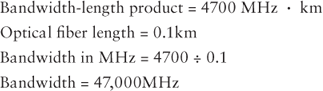
The steps to calculate the minimum effective modal bandwidth for 300 meters of OM4 optical fiber at a wavelength of 850nm are as follows:
- Bandwidth-length product = 4700 MHz · km
- Optical fiber length = 0.3km
- Bandwidth in MHz = 4700 ÷ 0.3
- Bandwidth = 15,666.67MHz
Calculate the Attenuation for a Length of Optical Fiber
The maximum allowable attenuation in an optical-fiber is defined in TIA-568-C.3 and ISO/IEC 11801.
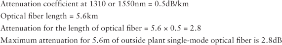
Refer to the following table and determine the maximum allowable attenuation for 5.6km of outside plant single-mode optical fiber.
| Optical fiber cable type | Wavelength (nm) | Maximum attenuation (dB/km) |
| 50/125μm multimode | 850 1300 |
3.5 1.5 |
| 62.5/125μm multimode | 850 1300 |
3.5 1.5 |
| Single-mode inside plant cable | 1310 1550 |
1.0 1.0 |
| Single-mode outside plant cable | 1310 1550 |
0.5 0.5 |
The maximum attenuation for outside plant single-mode optical fiber is the same for both wavelengths. The steps to calculate the maximum attenuation are as follows: