6
How to Develop an Alpha. II: A Case Study
By Hongzhi Chen
An alpha has multiple definitions. The most widely used definition we use is: a computer algorithm used to predict financial instruments’ future movements. Another commonly used term is alpha value, which is the value we assign to each instrument, proportional to the money we use to invest in it. As we talk about alpha, we generally refer to the first definition. When we talk about alpha value, we refer to the second.
Before we talk more about alpha design, let’s study a simple example to get a better understanding of what an alpha looks like.
Say we have $1M capital and want to invest continually in a portfolio consisting of two stocks: Google (GOOG) and Apple (AAPL). We need to know how to allocate our capital between these two stocks. If we do a daily rebalance of our portfolio, we need to predict the next few days’ return of each stock. How do we do this?
There are a lot of things that can affect the stock prices, such as trader behavior, news, fundamental change, insider behavior, etc. To make things simple, we can deconstruct the prediction process into two steps: first, we predict stock return using a single factor like news; second, we aggregate all different predictions.
As the first step, we will need a data loader to load news. Next, we need to figure out an algorithm to turn the text news into a vector whose values are the money we want to invest in each stock. If we predict the stock price will rise, we invest more in it; otherwise, we short more of it. The computer algorithm used to do this prediction is the so-called alpha.
In the previous example, suppose our algorithm gets the following value:
Alpha (GOOG) = 2
Alpha (AAPL) = –1
The values above are a ratio of 2 to –1. This means we want to hold twice as much of GOOG as we do of AAPL, and the positive sign means we want to hold a long position, while the negative sign means we want to hold a short position. Thus, using $1M of capital as an example, we want to long $1M of GOOG, and short $–0.5M of AAPL at the end of today’s trading. This example, of course, assumes zero transaction costs.
So the alpha model is actually an algorithm that transforms input data (price/volume, news, fundamental, etc.) into a vector, which is proportional to the money we want to hold in each instrument.
Alpha (input data) → alpha value vector
Now that we understand what an alpha means, let’s write our first alpha.
We will introduce more concepts along the way.
Above all, we need to define a universe, i.e. the set of financial instruments that we want to build the alpha model with. Let’s focus on the US equity market. There are different ways to do this, like using components of the S&P 500 index, using the most liquid 3,000 stocks, etc. Suppose we use the most liquid 3,000 stocks in the US as our research universe, call it TOP3000.
Next, we need an idea to predict the stock price. Behavioral finance states that, on the short-term horizon, the stock price tends to revert back due to the overreaction of the traders. How do we implement this idea? There are many ways to do it. For the purpose of demonstration, we will try a very simple implementation:
Alpha1 = –(close (today) – close (5_days_ago)) /close (5_days_ago)
This implementation means we assume the stock price will revert back to its price five days ago. If today’s price is lower than the price of five days ago, we want to long the stock and vice versa. We use the five days’ return as the amount of the money we want to hold. This means if the discrepancy is bigger in terms of return, we predict the reversion will be higher.
Now we get our first alpha, it’s really simple.
To test if this idea works, we need a simulator to do backtesting. We can use WebSim™ for this purpose.
Using WebSim™, we get the sample results for this alpha as shown in Figure 6.1.
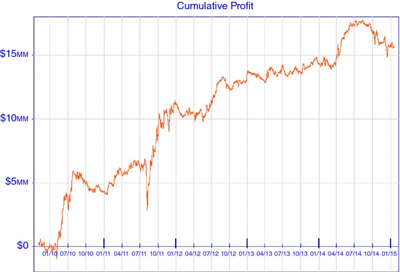
Figure 6.1 Sample simulation result of Alpha1 by WebSim™
There are some new concepts in Table 6.1, as shown on the following page. We list the most important ones we need to learn in order to evaluate an alpha.
Table 6.1 Evaluation of Alpha1 simulation graph
| Year | Booksize | PnL | Ann. return | Information ratio | Max drawdown | % profitable days | Daily turnover | Profit per $ traded |
| 2010 | 2.0E7 | 4.27E6 | 46.44% | 1.32 | 16.63% | 46.52% | 62.69% | 0.15 ¢ |
| 2011 | 2.0E7 | 6.93E6 | 68.70% | 1.42 | 39.22% | 50.79% | 64.72% | 0.21 ¢ |
| 2012 | 2.0E7 | 2.01E6 | 20.08% | 0.96 | 14.66% | 51.20% | 63.36% | 0.06 ¢ |
| 2013 | 2.0E7 | 1.04E6 | 10.34% | 0.60 | 9.22% | 46.83% | 63.26% | 0.03 ¢ |
| 2014 | 2.0E7 | 1.48E6 | 14.72% | 0.61 | 28.67% | 51.19% | 62.36% | 0.05 ¢ |
| 2015 | 2.0E7 | –158.21E3 | –32.96% | –1.38 | 4.65% | 41.67% | 64.34% | –0.10 ¢ |
| 2010 – 2015 | 2.0E7 | 15.57E6 | 31.20% | 1.00 | 39.22% | 49.28% | 63.30% | 0.10 ¢ |
Note: provided for illustrative purposes only
The backtesting is done from 2010 to 2015, so each row of the output lists the annual performance of that year. The total simulation booksize is always fixed to $20M; PnL is annual PnL.
Annual return is defined as:
Ann_return: = ann_pnl/(booksize/2)
It measures the profitability of the alpha. Information ratio is the single most important metric we will look at. It’s defined as:
Information_ratio: = (average daily return)/(daily volatility) * sqrt (256)
It measures the information in the alpha, which roughly means the stability of the alpha’s profitability; the higher the better. Max drawdown measures the loss from highest PnL point to lowest PnL point in percentage of booksize/2. Percent profitable measures the percentage of positive days in each year. Daily turnover measures how fast you rebalance your portfolio, and is defined as:
Daily_turnover: = (average dollars traded each day)/booksize
Profit per $ traded measures how much you made for each dollar you traded, and is defined as:
Profit_per_$_traded: = pnl/total_traded_dollar
For this alpha, the total information ratio is about 1 with a high return of about 30%, with a very high max drawdown of 39%. This means the risk is very high, so the PnL is not very stable. To reduce the max drawdown, we need to remove some risks. We can achieve this by using some risk neutralization techniques. Industry risk and market risk are the biggest risks for the equity market. We can remove them partially by requiring our portfolios to be always long/short balanced within each industry.
So basically, we adjust our alpha by requiring:
Alpha2 = Alpha1
Sum (Alpha2 value within same industry) = 0
By doing this, we get a new sample result as seen in Figure 6.2.
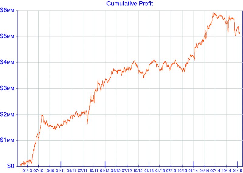
Figure 6.2 Sample simulation result of Alpha2 by WebSim™
As can be seen in Table 6.2, the information ratio is increased to 1.4, return is decreased to 10%, but max drawdown is decreased significantly to only 9%. This is a big improvement!
Table 6.2 Evaluation of Alpha2 simulation graph
| Year | Booksize | PnL | Ann. return | Information ratio | Max drawdown | % profitable days | Daily turnover | Profit per $ traded |
| 2010 | 2.0E7 | 1.59E6 | 17.30% | 2.44 | 5.44% | 51.30% | 63.73% | 0.05 ¢ |
| 2011 | 2.0E7 | 1.66E6 | 16.50% | 1.81 | 5.27% | 49.21% | 63.85% | 0.05 ¢ |
| 2012 | 2.0E7 | 518.24E3 | 5.18% | 0.90 | 6.66% | 55.20% | 63.12% | 0.02 ¢ |
| 2013 | 2.0E7 | 450.88E3 | 4.47% | 0.80 | 4.97% | 51.59% | 62.99% | 0.01 ¢ |
| 2014 | 2.0E7 | 1.11E6 | 11.02% | 1.24 | 8.73% | 53.17% | 62.86% | 0.04 ¢ |
| 2015 | 2.0E7 | –231.40E3 | –48.21% | –5.96 | 2.88% | 33.33% | 62.30% | –0.15 ¢ |
| 2010 – 2015 | 2.0E7 | 5.10E6 | 10.22% | 1.37 | 8.73% | 51.92% | 63.29% | 0.03 ¢ |
To further improve the alpha, we noticed that the magnitude of our alpha is five days’ return, which is not very accurate as a predictor. Maybe the relative size is more accurate as a predictor. So we next introduce the concept of rank. Rank means using the relative rank of the alpha value as the new alpha.
Alpha3 = rank (Alpha1)
Sum (Alpha3 value within same industry) = 0
The results are reflected in Figure 6.3.
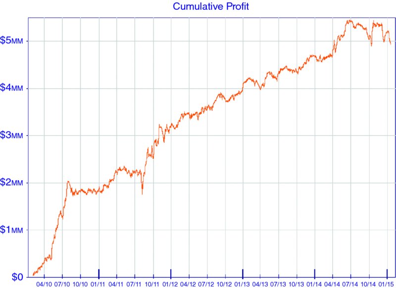
Figure 6.3 Sample simulation result of Alpha3 by WebSim™
As can be seen in Table 6.3, we get another significant improvement! Now performance looks much better, yet turnover is still a little high. We can try to decrease it by using decay. Decay means averaging your alpha signal within a time window.
Table 6.3 Evaluation of Alpha3 simulation result
| Year | Booksize | PnL | Ann. return | Information ratio | Max drawdown | % profitable days | Daily turnover | Profit per $ traded |
| 2010 | 2.0E7 | 1.83E6 | 19.94% | 3.43 | 3.11% | 56.52% | 59.43% | 0.07 ¢ |
| 2011 | 2.0E7 | 1.34E6 | 13.30% | 1.70 | 5.82% | 53.17% | 59.49% | 0.04 ¢ |
| 2012 | 2.0E7 | 801.74E3 | 8.02% | 1.89 | 1.93% | 55.20% | 58.94% | 0.03 ¢ |
| 2013 | 2.0E7 | 692.73E3 | 6.87% | 1.94 | 2.49% | 53.57% | 58.69% | 0.02 ¢ |
| 2014 | 2.0E7 | 518.06E3 | 5.14% | 0.93 | 5.43% | 52.38% | 59.20% | 0.02 ¢ |
| 2015 | 2.0E7 | –251.40E3 | –52.37% | –10.45 | 2.78% | 33.33% | 59.59% | –0.18 ¢ |
| 2010 – 2015 | 2.0E7 | 4.94E6 | 9.89% | 1.76 | 5.82% | 53.93% | 59.15% | 0.03 ¢ |
Basically, it means:
New_alpha = new_alpha + weighted_old_alpha
By trying three days’ decay in WebSim™, we get the chart as seen in Figure 6.4.
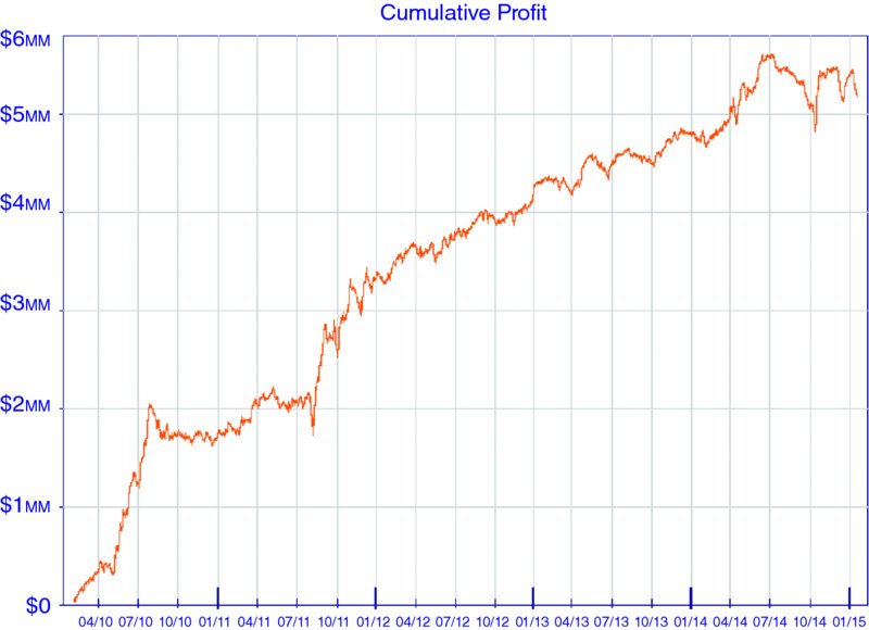
Figure 6.4 Sample simulation result of New_alpha by WebSim™
Table 6.4 looks great! Not only is turnover decreased, but information ratio, return, and drawdown are also improved!
Table 6.4 Evaluation of New_alpha simulation result
| Year | Booksize | PnL | Ann. return | Information ratio | Max drawdown | % profitable days | Daily turnover | Profit per $ traded |
| 2010 | 2.0E7 | 1.72E6 | 18.66% | 3.09 | 4.11% | 53.91% | 42.48% | 0.09 ¢ |
| 2011 | 2.0E7 | 1.61E6 | 15.94% | 2.01 | 4.87% | 51.19% | 42.28% | 0.08 ¢ |
| 2012 | 2.0E7 | 814.03E3 | 8.14% | 1.90 | 2.05% | 57.20% | 42.09% | 0.04 ¢ |
| 2013 | 2.0E7 | 643.29E3 | 6.38% | 1.88 | 2.48% | 54.76% | 41.87% | 0.03 ¢ |
| 2014 | 2.0E7 | 599.21E3 | 5.94% | 1.03 | 7.74% | 51.59% | 42.09% | 0.03 ¢ |
| 2015 | 2.0E7 | –194.34E3 | –40.49% | –7.20 | 2.58% | 33.33% | 41.82% | –0.19 ¢ |
| 2010 – 2015 | 2.0E7 | 5.19E6 | 10.39% | 1.82 | 7.74% | 53.53% | 42.15% | 0.05 ¢ |
We now know how to turn an alpha idea into an algorithm, and learned some techniques to improve it. You can think of more ways to improve it, just be creative.
This is basically how alpha research is done.1
The next step is to explore other ideas and data sets, hunting for something really unique. A unique idea is good since you can trade it before others do, potentially leading to more profit.
Good luck!