
31
Alpha Tutorials
By the WebSim™ Team
This chapter provides a selection of expression and python examples to get a new user started. It also has descriptions of some common alpha examples with a discussion on good practices to follow when building alphas.
ALPHA EXPRESSION EXAMPLES
Try the alpha expressions in Table 31.1 with different Universe, Delay, Neutralization, etc. settings.
Table 31.1 Sample alpha expressions
| Expression | Description |
| 1/close | Use inverse of daily close price as stock weights. More allocation of capital on the stocks with lower daily close prices. Similarly in the examples below, more allocation of capital on stocks with higher weights as defined in the “Expression” column. |
| volume/adv20 | Use relative daily volume to the average in the past 20 days as stock weights. |
| Correlation(close, open, 10) | Use correlation between daily close and open prices in the past 10 days as stock weights. |
| open | Use daily open price as stock weights. |
| (high + low)/2 - close | Use difference between average of daily high and low prices and daily close price as stock weights. |
| vwap < close ? high : low | Use daily high as stock weights if the stock closes higher than daily volume weighted average price (vwap), or otherwise use daily low as stock weights. |
| Rank(adv20) | Use rank of average daily volume in past 20 days (adv20) as stock weights. |
| Min(0.5*(open+close), vwap) | Use the less of open close average and vwap as stock weights. |
| Max(0.5*(high+low), vwap) | Use the greater of high low average and vwap as stock weights. |
| 1/StdDev(returns, 22) | Use inverse of standard deviation of stock returns in past 22 days as stock weights. |
| Sum(sharesout, 5) | Use sum of outstanding shares in past 5 days as stock weights. |
| Covariance(vwap, returns, 22) | Use covariance of vwap and returns for the past 22 days as stock weights. |
| 1/Abs(0.5*(open+close) - vwap) | Use absolute difference between open close average and vwap as stock weights. |
| Correlation(vwap, Delay(close, 1), 5) | Use correlation between vwap and previous day’s close for past 5 days as stock weights. |
| Delta(close, 5) | Use difference between daily close and close on the date 5 days earlier as stock weights. |
| Decay_linear(sharesout*vwap, 5) | Use linear decay of vwap multiplied by sharesout over the last 5 days as stock weights. |
| Decay_exp(close, 0.25, 5) | Use exponential decay of close with smoothing factor 0.25 over the last 5 days as stock weights. |
| Product(volume/sharesout, 5) | Use product of volume/sharesout ratio for the past 5 days as stock weights. |
| Tail(close/vwap, 0.9, 1.1, 1.0) | Use close/vwap ratio as stock weights if it is less than 0.9 or greater than 1.1, or otherwise use 1 as stock weights. |
| Sign(close-vwap) | Use 1 if close-vwap is positive or otherwise -1 as stock weights. |
| SignedPower (close-open, 0.5) | Use sqrt of absolute difference between close and open as stock weights. |
| Pasteurize(1/(close-open)) | Use inverse of close-open pasteurized (set to NaN if it is INF or if the underlying instrument is not in the universe) as stock weights. |
| Log(high/low) | Use natural logarithm of high/low ratio as stock weights. |
| IndNeutralize(volume*vwap, 1) | Use market neutralized volume*vwap product as stock weights. |
| Scale(close^0.5) | Use scaled sqrt of close (scaled such that the Book size is 1) as stock weights. |
| Ts_Min(open, 22) | Use minimum open over the last 22 days as stock weights. |
| Ts_Max(close, 22) | Use maximum open over the last 22 days as stock weights. |
| Ts_Rank(volume, 22) | Use rank of current volume over the past 22 days as stock weights. |
| Ts_Skewness(returns, 11) | Use skewness of returns over the last 11 days as stock weights. |
| Ts_Kurtosis(returns, 11) | Use kurtosis of returns over the last 11 days as stock weights. |
| Ts_Moment(returns, 3, 11) | Use 3rd central moment of returns over the last 11 days as stock weights. |
| CountNans((close-open)^0.5, 22) | Use number of NaN values in (close-open)^0.5 for the past 22 days as stock weights. |
| Step(1250)*close | Use close*Step(1250) product as stock weights. |
| Sum_i(Delta(close,i),i,4,6,2) | Use summation of Delta(close,i) over i from 4 to 6 step 2 as stock weights. |
| Call_i(Ts_Rank(x,5),x, close>vwap ? close : high) | Use Ts_Rank(x,5) as stock weights where x is daily close price if it’s higher than vwap, or otherwise use daily high price as stock weights. |
HOW TO CODE ALPHAS IN PYTHON
You should have good working knowledge of Python programming language to develop Python alphas on WebSim™. Useful links to online Python tutorials are given in Table 31.2.
Table 31.2 Links to online Python tutorials
The user should abide by the terms of use of the above-mentioned sites. The links are listed for user’s convenience only.
Imported Libraries
Keep in mind that any user-submitted Python code is always prefixed by WebSim™ with the following:
- import scipy as sp # python library that supplements numeric modules
- from numpy import * # library that contains N-dim array object, linear algebra, etc.
- import scipy.stats as ss # import statistical functions
- delay = 1 # alpha delay
- dr = WQSim_DataRegistry.Instance() # dr is initialized as data registry object
- # use dr.GetData() to access market data
- valid = dr.GetData_m_b("USA:TOP3000") # GetData_m_b() accesses Universe data. The result valid is a matrix of Boolean values that specifies which instruments are valid in the universe on a given day. The GetData_m_b() function is used to access data of type Boolean matrix(_m_b stands for matrix, boolean)
Accessing Data
WebSim™ application is enabled to access market data on the back end by using the Python code, GetDataon, the data registry. For example:
- shares_outstanding=dr.GetData("sharesout") # to access outstanding shares data
- ltDebt=dr.GetData("debt_lt") # for long-term debt data
- closePrice=dr.GetData("close") # for close price data
Generate() Function, Indices, and Alpha Expression
As explained before, the market data can be thought of as a matrix of values provided for each stock for every date the data is made available. The dates are mapped to date indices di and the instruments are mapped to instrument indices ii as shown in Table 31.3.
Table 31.3 Mapping dates to date indices di and instruments to instrument indices ii
| Dates | di(date index) | Instruments | ii(instr index) |
| 20100101 | 0 | MSFT | 0 |
| 20100102 | 1 | AAPL | 1 |
| 20100103 | 2 | PG | 2 |
| 20100104 | 3 | GOOG | 3 |
| 20100107 | 4 | AA | 4 |
| 20100108 | 5 | K | 5 |
| … | … | … | … |
Market data, e.g. close price, would be arranged in the form of a matrix as shown in Table 31.4.
Table 31.4 Market data arranged in the form of a matrix
| Instruments Dates |
MSFT (ii=0) |
HOG (ii=1) |
AAPL (ii=2) |
GOOG (ii=3) |
PG (ii=4) |
… |
| 20100104(di=0) | 30.95 | 25.46 | 214.01 | 626.75 | 61.12 | … |
| 20100105(di=1) | 30.96 | 25.65 | 214.38 | 623.99 | 61.14 | … |
| 20100106(di=2) | 30.77 | 25.59 | 210.97 | 608.26 | 60.85 | … |
| 20100107(di=3) | 30.452 | 25.8 | 210.58 | 594.1 | 60.52 | … |
| 20100108(di=4) | 30.66 | 25.53 | 211.98 | 602.02 | 60.44 | … |
| … | … | … | … | … | … | … |
Now to access Apple’s close price on date Jan 7, 2010, we need to use close(3,2).
The sole purpose of the Generate( ) function (should be implemented in your code) is to populate the resulting alpha vector with stock weights for every stock. The Generate function will evaluate the alpha expression for every date (it acts like a loop that iterates through all date indices), hence its arguments are di (which is the date index corresponding to the current date) and alpha (the resulting vector that needs to be filled). For example:
- closePrice = dr.GetData("close")
- def Generate(di,alpha):
- # Alpha expression goes here
Data can be accessed using dataname[di-delay,ii].
dataName[date index, instrument index] would give you the value of dataname, for that particular date, and that particular instrument. To assign expression to an alpha, use alpha[instrument index] = expression.
For example, alpha[ii] = dataname[di,ii].
An example alpha code to use close price data is given below:
- closePrice = dr.GetData("close")
- def Generate(di,alpha):
- alpha[:] = 1./closePrice[di-delay,:]
- # The above statement is equivalent to the expression '1/close'
- # “:” here refers to all instrument indices 0 <= ii< alpha.shape[0]
Since we are using the list-slicing functionality (“:”) of Python, it executes the expression for each instrument (corresponding column cell in the matrix).
Another example that uses returns data to define alpha[:] is given below:
- returnsMat = dr.GetData("returns")
- def Generate(di,alpha):
- alpha[:] = -(returnsMat[di-delay,:]) # reversion(returns always tends to mean)
To access data for an instrument over a certain window period, say n days, use dataname[di-delay-n: di-delay, ii]. An example for this is given below:
- closePrice = dr.GetData("close")
- def Generate(di,alpha):
- alpha[:] = mean(close[di-delay-10:di-delay,:], axis = 0) # taking the mean of the close price for the last 10 days
- alpha[:] = where(valid[di,:],alpha[:],nan) # valid check
The user should note that the window period chosen should be less that the number of lookback days (namely set to 256 days, by default). This value can be retrieved using Python function: Build.GetBackdays().
The last line is added as a validity check for values in the resultant alpha array. This will ensure that the values for instruments that don’t belong to the TOP3000 universe will be filtered out. Notice that this uses the valid variable, which was initialized as mentioned in the Python code header. This is explained further in the next section.
PYTHON ALPHA EXAMPLES
Here are several common examples of how Python can be used.
Using Multiple Data Simultaneously
The following example shows us how to access and use multiple data at the same time. Use vectorization wherever possible. Avoid using loops as they are slow. This example uses NumPy’s built-in math function (numpy.subtract is called automatically). Here, the alpha vector is assigned expression close – high.
- # Different data need different variables
- closePrice=dr.GetData("close")
- highPrice=dr.GetData("high")
- def Generate(di,alpha):
- alpha[:] = closePrice[di-delay,:] - highPrice[di-delay,:]
Using Custom-Defined Functions
The following py code shows us how to define custom functions and use them. It also uses the NumPy function numpy.where(). This should be used instead of loops to perform vector comparison.
- closePrice=dr.GetData("close")
- lowPrice=dr.GetData("low")
- def Generate(di,alpha):
- # np_max (defined below) can be called in this code
- alpha[:] = np_max(closePrice[di-delay,:], lowPrice[di-delay-1, :])
- # This is equivalent to the expression 'Max(close, Delay(low, 1))'
- def np_max(data1, data2):
- return where(data1 > data2, data1, data2) # numpy.where() performs vector comparison
Incorrect Way to Assign Alpha Values
- closePrice=dr.GetData("close")
- def Generate(di,alpha):
- alpha[:] = closePrice[di-delay,:] # equivalent to the expression 'close'
- alpha = ones(alpha.shape[0])
- # Tries to assign all ones to the alpha vector using numpy.ones
- # Notice the lack of [:] after “alpha.” This assigns a new object to alpha rather than modify the existing object alpha is pointing to. The effect of this statement is that WebSim™ loses track of the alpha vector
- alpha[:]=1./closePrice[di-delay,:] # equivalent to the expression “1/close”
- # This statement has no effect because of the statement before it. The final alpha value is “close” instead of “1/close”
Use of Valid Matrix
The valid matrix has a list of valid instruments (for example, 3,000 instruments for TOP3000) and is automatically available:
- closePrice=dr.GetData("close")
- def Generate(di,alpha):
- alpha[:] = 1./closePrice[di-delay,:]
- alpha[:] = onlyValid(alpha, di) # User defined function. Filters out values for invalid instruments
- def onlyValid(x, di):
- myValid = valid[di-delay, :] # myValid vector has yesterday’s valid values only
- return where(myValid, x, nan)
- # We use NumPy’s where() function to filter out invalid instruments Always assign numpy.nan() to filter out instruments. “0” is a valid alpha value
The above valid-check function can be inserted at the end of all your alpha codes as:
- alpha[:] = where(valid[di-delay,:],alpha[:],nan)
Using Statistics Functions Available in SciPy
A list of SciPy’s statistical functions can be found at SciPy.org. We will be using the scipy .rankdata() function here. This assigns ranks to alpha weight, dealing with ties appropriately.
- high=dr.GetData("high")
- def Generate(di,alpha):
- alpha[:] = ss.rankdata(high[di-delay, :]) # using SciPy’s rank function. The equivalent expression is Rank(high)
- alpha[:] = where(valid[di-delay,:],alpha[:],nan)
The above alpha expression ranks (on a scale from 0 to 1) adjusted High prices.
The following alpha example shows the usage of a SciPy function called scipy.kurtosis() on close price for 11 days.
- closePrice = dr.GetData("close")
- def Generate(di,alpha):
- alpha[:] = ss.kurtosis(close[di-delay-11:di-delay,:], axis = 0) # using SciPy’s kurtosis function. The equivalent expression is kurtosis(close,11)
- alpha[:] = where(valid[di-delay,:],alpha[:],nan)
The following alpha example shows the usage of a SciPy function called scipy.skewness() on returns for 10 days.
- returns = dr.GetData("returns")
- def Generate(di, alpha):
- alpha[:] = ss.skew (returns[di-delay-10:di-delay,:], axis = 0) # using SciPy’s skewness function. The expression is equivalent to skewness(returns,10)
- alpha[:] = where(valid[di-delay,:],alpha[:],nan)
Using Statistics Functions Available in NumPy
A list of NumPy’s statistical functions can be found here: NumPy.org.
The alpha example below shows usage of NumPy’s mean and standard deviation function numpy.std():
- closePrice = dr.GetData("close")
- def Generate(di,alpha):
- alpha[:] = mean(close[di-delay-5:di-delay,:], axis = 0)/std(close[di-delay-5:di-delay,:], axis = 0)
- # equivalent to expression [Sum(close,5)/5]/ StdDev(close,5)
- alpha[:] = where(valid[di,:],alpha[:],nan)
The alpha example below shows usage of NumPy’s maximum function numpy.amax():
- closePrice = dr.GetData("close")
- def Generate(di, alpha):
- alpha[:] = amax(close[di-delay-20:di-delay,:], axis = 0) # finds maximum close over past 20 days
- alpha[:] = where(valid[di,:],alpha[:],nan)
Accessing and Using Industry Data
- closePrice = dr.GetData("close")
- industry = dr.GetData("industry") # accessing industry data
- def Generate(di,ti,alpha):
- ind = unique(where(industry[di-delay, :] > 0, industry[di-delay, :], 0))
- indclose = zeros(ind.shape[0]) # initialize a NumPy array full of zeros
- for i in xrange(ind.shape[0]):
- indclose[i] = mean(where((industry[di-delay, :] == ind[i]) * (valid[di-delay, :]), closePrice[di-delay, :], 0))
- alpha[:] = where( (industry[di-delay, :] == ind[i]) * (valid[di-delay,:]), indclose[i], alpha[:])
Industry data here is a NumPy array of indices assigned for every available industry. Industries such as Forestry, Metal Mining, Electrical Work, Meat Packing Plants, Textile Mills, Book Printing, etc., have indices assigned to them. The alpha above shows how this industry data can be accessed and used.
Table 31.5 shows a sample of instrument indices, industry indices (values of industry[di-delay,ii]), close data.
Table 31.5 Sample instrument indices, industry indices (values of industry [di-delay, ii], close data
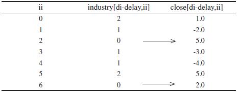
For the above alpha example, the industry close array values for each “I” will be as follows:
- Since indclose[i] = Average of closePrice[di-delay,ii] if current instrument belongs to current industry,
- indclose[0] = (5.0+2.0)/2 = 3.5 (shown in table)
- indclose[1] = (-2.0-3.0-4.0)/3 = -3
- indclose[2] = (1.0+5.0)/2 = 3
- Then alpha[ii] is assigned the value of indclose[industry[di-delay,ii]]
Note that you can also access and use sector and subindustry data using dr.GetData() in your alphas.
Simple Linear Regression Model
In the code given below, five days’ values of close price and vwap as training sample are used to calculate regression weights w1 and w2.
- Model formula: close[di] = w1 * close[di-1] + w2* vwap[di-1]
- closePrice=dr.GetData("close")
- vwapPrice=dr.GetData("vwap")
- def Generate(di,alpha):
- CloseX=zeros((5,closePrice.shape[1])) # initialize NumPy array
- CloseY=zeros((5,closePrice.shape[1]))
- VwapX=zeros((5,vwapPrice.shape[1]))
- for dnum in xrange(5):
- CloseX[dnum,:]=closePrice[di-delay-dnum-1,:]
- VwapX[dnum,:]=vwapPrice[di-delay-dnum-1,:]
- CloseY[dnum,:]= closePrice[di-delay-dnum,:]
- for ii in xrange(alpha.shape[0]):
- SampleX=hstack((CloseX[:,[ii]],VwapX[:,[ii]])) # NumPy function hstack() stacks arrays in sequence horizontally(column wise)
- ParaX=LinearRegres(SampleX,CloseY[:,[ii]])
- alpha[ii]=float(ParaX[0])*closePrice[di-delay,ii]+float(ParaX[1])*vwapPrice[di-delay,ii] # equivalent to expression: w1 * close[di-1] + w2* vwap[di-1]
- alpha[:] = where(valid[di,:],alpha[:],nan)
- def LinearRegres(xArr,yArr):
- xMat=matrix(xArr)
- yMat=matrix(yArr)
- xTx= xMat.T*xMat
- res=linalg.det(xTx) # NumPy’s linear algebra function that computes the determinant of the array
- if res==0.0 or isnan(res): # if res is 0 or nan
- return matrix([[nan],[nan]])
- else:
- return xTx.I*(xMat.T*yMat) # matrix.I takes the matrix’s inverse and matrix.T takes its transpose.