
Chapter 6. Solution Of Viscous-Flow Problems
6.1 Introduction
THE previous chapter contained derivations of the relationships for the conservation of mass and momentum—the equations of motion—in rectangular, cylindrical, and spherical coordinates. All the experimental evidence indicates that these are indeed the most fundamental equations of fluid mechanics, and that in principle they govern any situation involving the flow of a Newtonian fluid. Unfortunately, because of their all-embracing quality, their solution in analytical terms is difficult or impossible except for relatively simple situations. However, it is important to be aware of these “Navier-Stokes equations,” for the following reasons:
1. They lead to the analytical and exact solution of some simple, yet important problems, as will be demonstrated by examples in this chapter.
2. They form the basis for further work in other areas of chemical engineering.
3. If a few realistic simplifying assumptions are made, they can often lead to approximate solutions that are eminently acceptable for many engineering purposes. Representative examples occur in the study of boundary layers, waves, lubrication, coating of substrates with films, and inviscid (irrotational) flow.
4. With the aid of more sophisticated techniques, such as those involving power series and asymptotic expansions, and particularly computer-based numerical methods (as implemented by CFD or computational fluid dynamics software such as Fluent and COMSOL), they can lead to the solution of moderately or highly advanced problems, such as those involving injection-molding of polymers and even the incredibly difficult problem of weather prediction.
The following sections present exact solutions of the equations of motion for several relatively simple problems in rectangular, cylindrical, and spherical coordinates, augmented by a couple of CFD examples. Throughout, unless otherwise stated, the flow is assumed to be steady, laminar, and Newtonian, with constant density and viscosity. Although these assumptions are necessary in order to obtain solutions, they are nevertheless realistic in several instances.
The reader is cautioned that probably a majority of industrial processes involve turbulent flow, which is more complicated, and for this reason sometimes receives scant attention in university courses. The author has seen instances in which erroneous assumptions of laminar flow have led to answers that are wildly inaccurate.
All of the examples in this chapter are characterized by low Reynolds numbers. That is, the viscous forces are much more important than the inertial forces, and are usually counterbalanced by pressure or gravitational effects. Typical applications occur in microfluidics (involving tiny channels—see Chapter 12) and in the flow of high-viscosity polymers. Situations in which viscous effects are relatively unimportant will be discussed in Chapter 7.
Solution procedure
The general procedure for solving each problem involves the following steps:
1. Make reasonable simplifying assumptions. Almost all of the cases treated here will involve steady incompressible flow of a Newtonian fluid in a single coordinate direction. Further, gravity may or may not be important, and a certain amount of symmetry may be apparent.
2. Write down the equations of motion—both mass (continuity) and momentum balances—and simplify them according to the assumptions made previously, striking out terms that are zero. Typically, only a very few terms—perhaps only one in some cases—will remain in each differential equation. The simplified continuity equation usually yields information that can subsequently be used to simplify the momentum equations.
3. Integrate the simplified equations in order to obtain expressions for the dependent variables such as velocities and pressure. These expressions will usually contain some, as yet, arbitrary constants—typically two for the velocities (since they appear in second-order derivatives in the momentum equations) and one for the pressure (since it appears only in a first-order derivative).
4. Invoke the boundary conditions in order to evaluate the constants appearing in the previous step. For pressure, such a condition usually amounts to a specified pressure at a certain location—at the inlet of a pipe, or at a free surface exposed to the atmosphere, for example. For the velocities, these conditions fall into either of the following classifications:
(a) Continuity of the velocity, amounting to a no-slip condition. Thus, the velocity of the fluid in contact with a solid surface typically equals the velocity of that surface—zero if the surface is stationary.1 And, for the few cases in which one fluid (A, for example) is in contact with another immiscible fluid (B), the velocity in fluid A equals the velocity in fluid B at the common interface.
1 In a few exceptional situations there may be lack of adhesion between the fluid and surface, in which case slip can occur. Also see Example 12.4, in which electroosmosis gives the illusion of slip.
(b) Continuity of the shear stress, usually between two fluids A and B, leading to the product of viscosity and a velocity gradient having the same value at the common interface, whether in fluid A or B. If fluid A is a liquid, and fluid B is a relatively stagnant gas, which—because of its low viscosity— is incapable of sustaining any significant shear stress, then the common shear stress is effectively zero.
5. At this stage, the problem is essentially solved for the pressure and velocities. Finally, if desired, shear-stress distributions can be derived by differentiating the velocities in order to obtain the velocity gradients; numerical predictions of process variables can also be made.
Types of flow
Two broad classes of viscous flow will be illustrated in this chapter:
1. Poiseuille flow, in which an applied pressure difference causes fluid motion between stationary surfaces.
2. Couette flow, in which a moving surface drags adjacent fluid along with it and thereby imparts a motion to the rest of the fluid.
Occasionally, it is possible to have both types of motion occurring simultaneously, as in the screw extruder analyzed in Example 6.5.
6.2 Solution of the Equations of Motion in Rectangular Coordinates
The remainder of this chapter consists almost entirely of a series of worked examples, illustrating the above steps for solving viscous-flow problems.
Fig. E6.1.1. Geometry for flow through a rectangular duct. The spacing between the plates is exaggerated in relation to their length.
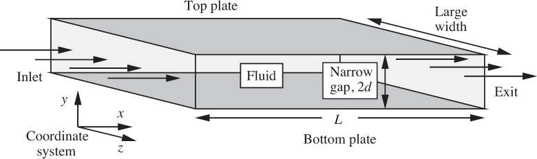
Fig. E6.1.1 shows a fluid of viscosity μ that flows in the x direction between two rectangular plates, whose width is very large in the z direction when compared to their separation in the y direction. Such a situation could occur in a die when a polymer is being extruded at the exit into a sheet, which is subsequently cooled and solidified. Determine the relationship between the flow rate and the pressure drop between the inlet and exit, together with several other quantities of interest.
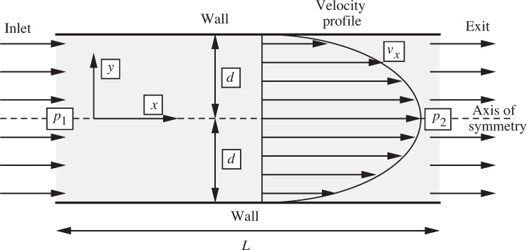
Fig. E6.1.2. Geometry for flow through a rectangular duct.
Simplifying assumptions
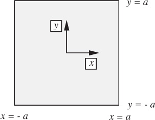
The situation is analyzed by referring to a cross section of the duct, shown in Fig. E6.1.2, taken at any fixed value of z. Let the depth be 2d (±d above and below the centerline or axis of symmetry y = 0), and the length L. Note that the motion is of the Poiseuille type, since it is caused by the applied pressure difference (p1 − p2). Make the following fairly realistic assumptions about the flow:
1. As already stated, it is steady and Newtonian, with constant density and viscosity. (These assumptions will often be taken for granted, and not restated, in later problems.)
2. Entrance effects can be neglected, so that the flow is fully developed, in which case there is only one nonzero velocity component—that in the direction of flow, vx. Thus, vy = vz =0.
3. Since, in comparison with their spacing, 2d, the plates extend for a very long distance in the z direction, all locations in this direction appear essentially identical to one another. In particular, there is no variation of the velocity in the z direction, so that ∂vx/∂z =0.
4. Gravity acts vertically downward; hence, gy = −g and gx = gz =0.
5. The velocity is zero in contact with the plates, so that vx =0 at y = ±d.
Continuity
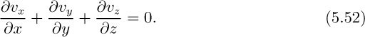
Start by examining the general continuity equation, (5.48):

which, in view of the constant-density assumption, simplifies to Eqn. (5.52):
But since vy = vz =0:
so vx is independent of the distance from the inlet, and the velocity profile will appear the same for all values of x. Since ∂vx/∂z = 0 (assumption 3), it follows that vx = vx(y) is a function of y only.
Momentum balances
With the stated assumptions of a Newtonian fluid with constant density and viscosity, Eqn. (5.73) gives the x, y, and z momentum balances:
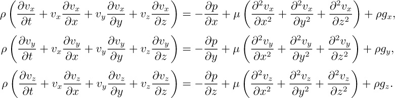
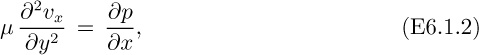
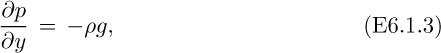
With vy = vz = 0 (from assumption 2), ∂vx/∂x = 0 [from the simplified continuity equation, (E6.1.1)], gy = −g, gx = gz = 0 (assumption 4), and steady flow (assumption 1), these momentum balances simplify enormously, to:
Pressure distribution
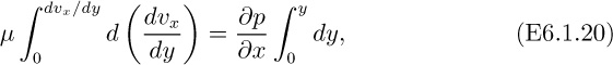
The last of the simplified momentum balances, Eqn. (E6.1.4), indicates no variation of the pressure across the width of the system (in the z direction), which is hardly a surprising result. When integrated, the second simplified momentum balance, Eqn. (E6.1.3), predicts that the pressure varies according to:

Observe carefully that since a partial differential equation is being integrated, we obtain not a constant of integration, but a function of integration, f(x).
Assume—to be verified later—that ∂p/∂x is constant, so that the centerline pressure (at y = 0) is given by a linear function of the form:
The constants a and b may be determined from the inlet and exit centerline pressures:
leading to:
Thus, the centerline pressure falls linearly from p1 at the inlet to p2 at the exit:
so that the complete pressure distribution is
That is, the pressure declines linearly, both from the bottom plate to the top plate, and also from the inlet to the exit. In the majority of applications, 2d ≪ L, and the relatively small pressure variation in the y direction is usually ignored. Thus, p1 and p2, although strictly the centerline values, are typically referred to as the inlet and the exit pressures, respectively.
Velocity profile
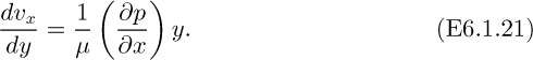
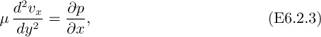
Since, from Eqn. (E6.1.1), vx does not depend on x, ∂2vx/∂y2 appearing in Eqn. (E6.1.2) becomes a total derivative, so this equation can be rewritten as:
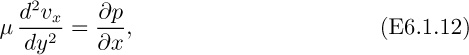
which is a second-order ordinary differential equation, in which the pressure gradient will be shown to be uniform between the inlet and exit, being given by:
A minus sign is used on the left-hand side, since ∂p/∂x is negative, thus rendering both sides of Eqn. (E6.1.13) as positive quantities.
Equation (E6.1.12) can be integrated twice, in turn, to yield an expression for the velocity. After multiplication through by dy, a first integration gives:

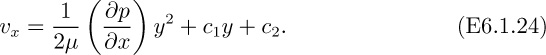
A second integration, of Eqn. (E6.1.14), yields:

The two constants of integration, c1 and c2, are determined by invoking the boundary conditions:

leading to:

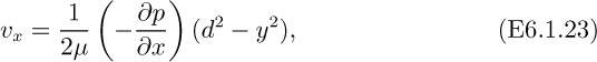
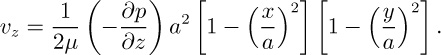
Eqns. (E6.1.15) and (E6.1.18) then furnish the velocity profile:
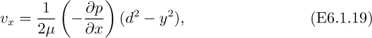
in which −∂p/∂x and (d2 − y2) are both positive quantities. The velocity profile is parabolic in shape, and is shown in Fig. E6.1.2.
Alternative integration procedure
Observe that we have used indefinite integrals in the above solution, and have employed the boundary conditions to determine the constants of integration. An alternative approach would again be to integrate Eqn. (E6.1.12) twice, but now to involve definite integrals by inserting the boundary conditions as limits of integration.
Thus, by separating variables, integrating once, and noting from symmetry about the centerline that dvx/dy =0 at y = 0, we obtain:
or:
A second integration, noting that vx = 0 at y = d (zero velocity in contact with the upper plate—the no-slip condition) yields:

That is:
in which two minus signs have been introduced into the right-hand side in order to make quantities in both pairs of parentheses positive. This result is identical to the earlier Eqn. (E6.1.19). The student is urged to become familiar with both procedures, before deciding on the one that is individually best suited.
Also, the reader who is troubled by the assumption of symmetry of vx about the centerline (and by never using the fact that vx = 0 at y = −d), should be reassured by an alternative approach, starting from Eqn. (E6.1.15):
Application of the two boundary conditions, vx =0 at y = ±d, gives
leading again to the velocity profile of Eqn. (E6.1.19) without the assumption of symmetry.
Volumetric flow rate
Integration of the velocity profile yields an expression for the volumetric flow rate Q per unit width of the system. Observe first that the differential flow rate through an element of depth dy is dQ = vxdy, so that:

Since from an overall macroscopic balance Q is constant, it follows that ∂p/∂x is also constant, independent of distance x; the assumptions made in Eqns. (E6.1.6) and (E6.1.13) are therefore verified. The mean velocity is the total flow rate per unit depth:

and is therefore two-thirds of the maximum velocity, vxmax, which occurs at the centerline, y =0.
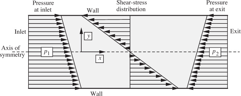
Fig. E6.1.3. Pressure and shear-stress distributions.
Shear-stress distribution
Finally, the shear-stress distribution is obtained by employing Eqn. (5.60):
By substituting for vx from Eqn. (E6.1.15) and recognizing that vy = 0, the shear stress is:

Referring back to the sign convention expressed in Fig. 5.12, the first minus sign in Eqn. (E6.1.28) indicates for positive y that the fluid in the region of greater y is acting on the region of lesser y in the negative x direction, thus trying to retard the fluid between it and the centerline, and acting against the pressure gradient. Representative distributions of pressure and shear stress, from Eqns. (E6.1.11) and (E6.1.28), are sketched in Fig. E6.1.3. More precisely, the arrows at the left and right show the external pressure forces acting on the fluid contained between x =0 and x = L.
6.3 Alternative Solution Using a Shell Balance
Because the flow between parallel plates was the first problem to be examined, the analysis in Example 6.1 was purposely very thorough, extracting the last “ounce” of information. In many other applications, the velocity profile and the flow rate may be the only quantities of prime importance. On the average, therefore, subsequent examples in this chapter will be shorter, concentrating on certain features and ignoring others.
The problem of Example 6.1 was solved by starting with the completely general equations of motion and then simplifying them. An alternative approach involves a direct momentum balance on a differential element of fluid—a “shell”—as illustrated in Example 6.2.
Employ the shell-balance approach to solve the same problem that was studied in Example 6.1.
Assumptions
The necessary “shell” is in reality a differential element of fluid, as shown in Fig. E6.2. The element, which has dimensions of dx and dy in the plane of the diagram, extends for a depth of dz (any other length may be taken) normal to the plane of the diagram.
Fig. E6.2. Momentum balance on a fluid element.
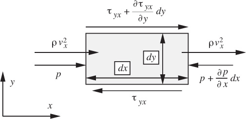
If, for the present, the element is taken to be a system that is fixed in space, there are three different types of rate of x momentum transfer to it:
1. A convective transfer of ![]() in through the left-hand face, and an identical amount out through the right-hand face. Note here that we have implicitly assumed the consequences of the continuity equation, expressed in Eqn. (E6.1.1), that vx is constant along the duct.
in through the left-hand face, and an identical amount out through the right-hand face. Note here that we have implicitly assumed the consequences of the continuity equation, expressed in Eqn. (E6.1.1), that vx is constant along the duct.
2. Pressure forces on the left- and right-hand faces. The latter will be smaller, because ∂p/∂x is negative in reality.
3. Shear stresses on the lower and upper faces. Observe that the directions of the arrows conform strictly to the sign convention established in Section 5.6. A momentum balance on the element, which is not accelerating, gives:
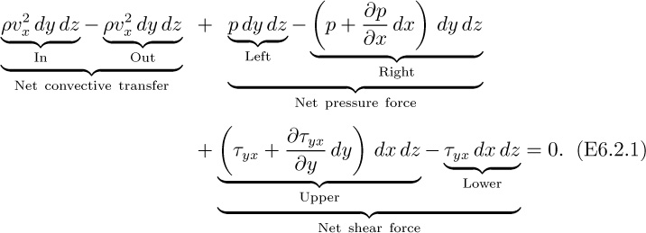
The usual cancellations can be made, resulting in:

in which the total derivative recognizes that the shear stress depends only on y and not on x. Substitution for τyx from Eqn. (5.60) with vy = 0 gives:
which is identical with Eqn. (E6.1.12) that was derived from the simplified Navier-Stokes equations. The remainder of the development then proceeds as in the previous example. Note that the convective terms can be sidestepped entirely if the momentum balance is performed on an element that is chosen to be moving with the fluid, in which case there is no flow either into or out of it.
The choice of approach—simplifying the full equations of motion, or performing a shell balance—is very much a personal one, and we have generally opted for the former. The application of the Navier-Stokes equations, which are admittedly rather complicated, has the advantages of not “reinventing the (momentum balance) wheel” for each problem, and also of assuring us that no terms are omitted. Conversely, a shell balance has the merits of relative simplicity, although it may be quite difficult to perform convincingly for an element with curved sides, as would occur for the problem in spherical coordinates discussed in Example 6.8.
This section concludes with another example problem, which illustrates the application of two further boundary conditions for a liquid, one involving it in contact with a moving surface, and the other at a gas/liquid interface where there is a condition of zero shear.
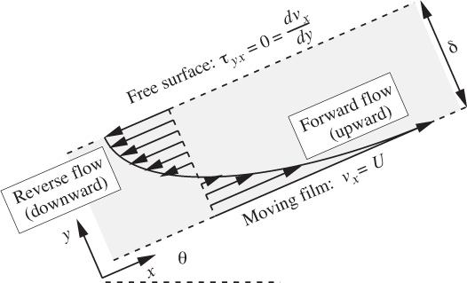
Fig. E6.3.1 shows a coating experiment involving a flat photographic film that is being pulled up from a processing bath by rollers with a steady velocity U at an angle θ to the horizontal. As the film leaves the bath, it entrains some liquid, and in this particular experiment it has reached the stage where: (a) the velocity of the liquid in contact with the film is vx = U at y = 0, (b) the thickness of the liquid is constant at a value δ, and (c) there is no net flow of liquid (as much is being pulled up by the film as is falling back by gravity). (Clearly, if the film were to retain a permanent coating, a net upwards flow of liquid would be needed.)
Fig. E6.3.1. Liquid coating on a photographic film.

Perform the following tasks:
1. Write down the differential mass balance and simplify it.
2. Write down the differential momentum balances in the x and y directions. What are the values of gx and gy in terms of g and θ? Simplify the momentum balances as much as possible.
3. From the simplified y momentum balance, derive an expression for the pressure p as a function of y, ρ, δ, g, and θ, and hence demonstrate that ∂p/∂x = 0. Assume that the pressure in the surrounding air is zero everywhere.
4. From the simplified x momentum balance, assuming that the air exerts a negligible shear stress τyx on the surface of the liquid at y = δ, derive an expression for the liquid velocity vx as a function of U, y, δ, and α, where α = ρg sin θ/μ.
5. Also derive an expression for the net liquid flow rate Q (per unit width, normal to the plane of Fig. E6.3.1) in terms of U, δ, and α. Noting that Q = 0, obtain an expression for the film thickness δ in terms of U and α.
6. Sketch the velocity profile vx, labeling all important features.
Assumptions and continuity
The following assumptions are reasonable:
1. The flow is steady and Newtonian, with constant density ρ and viscosity μ.
2. The z direction, normal to the plane of the diagram, may be disregarded entirely. Thus, not only is vz zero, but all derivatives with respect to z, such as ∂vx/∂z, are also zero.
3. There is only one nonzero velocity component, namely, that in the direction of motion of the photographic film, vx. Thus, vy = vz =0.
4. Gravity acts vertically downwards.
Because of the constant-density assumption, the continuity equation, (5.48), simplifies, as before, to:
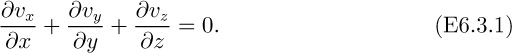
But since vy = vz = 0, it follows that
so vx is independent of distance x along the film. Further, vx does not depend on z (assumption 2); thus, the velocity profile vx = vx(y) depends only on y and will appear the same for all values of x.
Momentum balances
With the stated assumptions of a Newtonian fluid with constant density and viscosity, Eqn. (5.73) gives the x and y momentum balances:

Noting that gx = −g sin θ and gy = −g cos θ, these momentum balances simplify to:
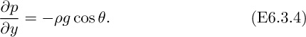
Integration of Eqn. (E6.3.4), between the free surface at y = δ (where the gauge pressure is zero) and an arbitrary location y (where the pressure is p) gives:

so that:
Note that since a partial differential equation is being integrated, a function of integration, f(x), is again introduced. Another way of looking at it is to observe that if Eqn. (E6.3.6) is differentiated with respect to y, we would recover the original equation, (E6.3.4), because ∂f(x)/∂y =0.
However, since p =0 at y = δ (the air/liquid interface) for all values of x, the function f(x) must be zero. Hence, the pressure distribution:
shows that p is not a function of x.
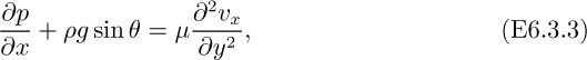
In view of this last result, we may now substitute ∂p/∂x = 0 into the x-momentum balance, Eqn. (E6.3.3), which becomes:
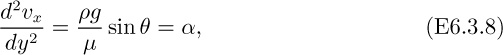
in which the constant α has been introduced to denote ρg sin θ/μ. Observe that the second derivative of the velocity now appears as a total derivative, since vx depends on y only.
A first integration of Eqn. (E6.3.8) with respect to y gives:
The boundary condition of zero shear stress at the free surface is now invoked:


A second integration, of Eqn. (E6.3.9) with respect to y, gives:
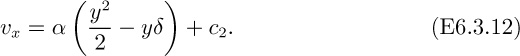
The second constant of integration, c2, can be determined by using the boundary condition that the liquid velocity at y = 0 equals that of the moving photographic film. That is, vx = U at y = 0, yielding c2 = U; thus, the final velocity profile is:
Observe that the velocity profile, which is parabolic, consists of two parts:
1. A constant and positive part, arising from the film velocity, U.
2. A variable and negative part, caused by gravity, which reduces vx at increasing distances y from the film and eventually causes it to become negative.
Fig. E6.3.2. Velocity profile in thin liquid layer on moving photographic film for the case of zero net liquid flow rate.
Exactly how much of the liquid is flowing upwards, and how much downwards, depends on the values of the variables U, δ, and α. However, we are asked to investigate the situation in which there is no net flow of liquid—that is, as much is being pulled up by the film as is falling back by gravity. In this case:

giving the thickness of the liquid film as:

The velocity profile for this case of Q = 0 is shown in Fig. E6.3.2.
This problem is one of the few instances in this book in which we investigate transient or unsteady-state fluid flow. It illustrates how momentum is transferred under the diffusive influence of viscosity.
Fig. E6.4.1. Region of liquid being studied, with the four COMSOL boundary conditions.
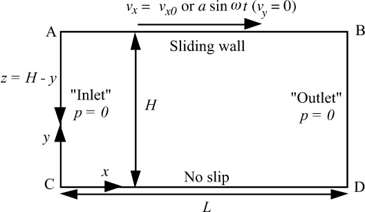
As shown in Fig. E6.4.1, consider a liquid of density ρ = 1 g/cm3 and viscosity μ (whose values will be given later), contained between two parallel plates AB and CD of length L = 2 cm and separation H = 1 cm. The lower plate CD is stationary, and the upper plate AB can undergo two types of movement:
1. At time t = 0, it is suddenly set in motion with a constant x-velocity vx = vx0. In our problem, vx0 = 1 cm/s and μ =0.5 g/cm s = 0.5 P.
2. At time t = 0, it is oscillated to the right and left in such a way that its x-velocity varies with time according to vx0 = a sin ωt. In our problem the amplitude a = 1 cm/s, the angular velocity ω =2π s−1, and the viscosity may be either μ =0.1 or 0.5 P.
Very similar types of motion occur in concentric-cylinder viscometers, as in Figs. 1.1 and 11.13(b), although with smaller moving-surface separations.
Use COMSOL to investigate how vx varies between the midpoints of the lower and upper plates at different times, and interpret the results. If needed, further details of the implementation of COMSOL are given in Chapter 14. All mouse-clicks are left-clicks (the same as Select) unless specifically denoted as right-click (R).
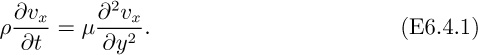
Note that COMSOL will employ the full Navier-Stokes and continuity equations in its solution. However, because the only nonzero velocity component is vx, the following familiar diffusion-type equation is effectively being solved:
Solution—Case 1 (Constant Upper-Plate Velocity)
Select the Physics
1. Open COMSOL and L-click Model Wizard, 2D, Fluid Flow (the little rotating triangle is called a “glyph”), Single-Phase Flow, Laminar Flow, Add. Note the symbols used by COMSOL—u, v, w for velocity components and p for pressure.
2. L-click Study, Time Dependent, Done.
Define the Parameters
3. R-click Global Definitions and select Parameters. In the Settings window to the right of the Model Builder window enter the parameter vx0 in the Name column and its value and units, 1 [cm/s], in the Expression column. Similarly, define L = 2 [cm], H = 1 [cm], rho1 = 1 [g/cm3], and mu1 = 0.5 [g/cm/s].
Establish the Geometry
4. R-click Geometry and select Rectangle. Note the default is based on the lower left corner being at (0, 0). Enter the values for Width and Height as L and H. L-click Build Selected.
Define the Fluid Properties
5. R-click the Materials node within Component 1 and select Blank Material. Note that the new material will have the required material parameters based on the physics of the problem. Enter the parameters rho1 and mu1 as the values for Density and Dynamic viscosity.
Define the Boundary Conditions
6. L-click Laminar Flow, Wall 1 and note the default No Slip boundary conditions that are highlighted.
7. R-click the Laminar Flow node and select Inlet to define an inlet boundary condition, and L-click the left boundary (#1) to select it as the inlet. Note that clicking on a boundary will change its color from red to blue. Within the Settings window L-click the dropdown box in the Boundary Condition node to select Pressure (equal to zero), deselect Suppress backflow, and leave Normal flow checked. R-click the Laminar Flow node and select Outlet, and L-click the right boundary (#4) to select it as the outlet, with zero pressure, Normal flow checked, and Suppress backflow unchecked. R-click the Laminar Flow node and L-click Wall. Select the top boundary (again changing from red to blue), and within the Settings window change the Boundary Condition from No Slip to Sliding wall. Enter vx0 as the value for the tangential velocity Uw.
Create the Mesh and Solve the Problem
8. L-click the Mesh node and change the Element Size in the Settings window to Fine. L-click Build All to construct the mesh. R-click Mesh 1 and Statistics will show that the mesh contains approximately 4,000 elements.
9. L-click the Study 1 little triangular glyph, and then select the Step 1 Time Dependent node and define the output range segments using the range function. For the requested output times, enter the three ranges as: range(0.0, 0.01, 0.1) range(0.2, 0.1, 0.5) range(1.0, 0.5, 2.0).
10. R-click the Study node and select Compute, which gives (after about 15 seconds) a surface plot of the magnitudes of the velocities—from low near the bottom (blue), medium at the middle (turquoise), and high near the top (red).
11. Save your results occasionally—for example, in the file Ex6.4-11.mph.
Display the Results (Case 1)
12. Create a data set at the midpoint in the y-direction. R-click the Data Sets node within the Results tree and select Cut Line 2D. In the Settings window enter the values (L/2, 0) and (L/2, H) for Points 1 and 2. L-click Plot near the top of the Settings window to display the cut line.
13. R-click Results and L-click 1D Plot Group. In the Settings window, Left-click the dropdown dialog and change the data set to Cut Line 2D 1, which was created above. Change the Time selection to “From list” and select the desired individual plot times by holding down the CTRL key (Command on a Mac) and then L-clicking on the individual values 0.01, 0.02, 0.05, 0.1, 0.2, 0.5, and 2.0.
Fig. E6.4.2. Plot of vx (m/s) against distance y (m) from the midpoint of the lower plate to the midpoint of the upper plate, for the indicated values of time (s).

14. R-click the 1D Plot Group 3 and select Line Graph. Within the Settings window enter the variable for the x-component of velocity, u, in the Expression field.
15. Expand the Coloring and Style section by L-clicking the triangular glyph to the left. Change the Color option to Black by L-clicking the dropdown dialog box.
16. L-click Plot in the Settings window to update the plot. Save in Ex6.4-16.mph or similar.
Discussion of Case 1 (Constant Upper-Plate Velocity)
Fig. E6.4.2 shows how the velocity vx varies with distance y from the lower plate at various times. The result is a classical case of diffusion—in this instance, of x-momentum (generated by the motion of the upper plate, which moves at 1 cm/s), into the liquid below it. For the smallest time plotted (t =0.01 s), most of the liquid, from y = 0 to 0.7 cm, is essentially undisturbed, followed by a rising vx between y = 0.7 and 1 cm. For early times (or for an infinitely deep liquid), before the influence of the lower plate is felt, there is an analytical solution:
in which z = H − y is the downwards distance from the upper plate, ν = μ/ρ is the kinematic viscosity, and erfc denotes the complementary error function.
As time increases, more and more of the liquid is set into motion by the diffusion of x-momentum from the upper plate. Eventually—theoretically at t = ∞ but effectively at a time of about 2 s—a steady state is reached, in which the shear stress exerted by the upper plate is counterbalanced by the shear stress in the opposite direction from the stationary lower plate. Since the velocity profile is linear, dvx/dy is constant; thus, these shear stresses are equal (and opposite) because they are both given by τyx = μdvx/dy.
Solution—Case 2 (Oscillating Upper-Plate Velocity)
17. Now solve the oscillatory surface time-dependent problem by first saving the model under a new name, such as Ex6.4-17.mph (or a file name of your choice).
18. Follow Step 3 above (Parameters under Global Definitions) to add the parameters for a and omega with values 1.0 [cm/s] and 2*pi [1/s]. Also update the viscosity by changing the value for mu1 to 0.1 [g/cm/s].
19. Update the top wall boundary condition, Wall 2. L-click Laminar Flow, Wall 2 and enter the tangential velocity value a*sin(omega*t).
20. Update the requested output times. L-click the Study 1, Step 1 Time Dependent node and enter the ranges as: range(0, 2, 18) range(19, 0.25, 20).
21. R-click the Study 1 node and select Compute. The solution took about 100 seconds on the author’s computer. The result is a surface plot showing velocity magnitudes, not needed here.
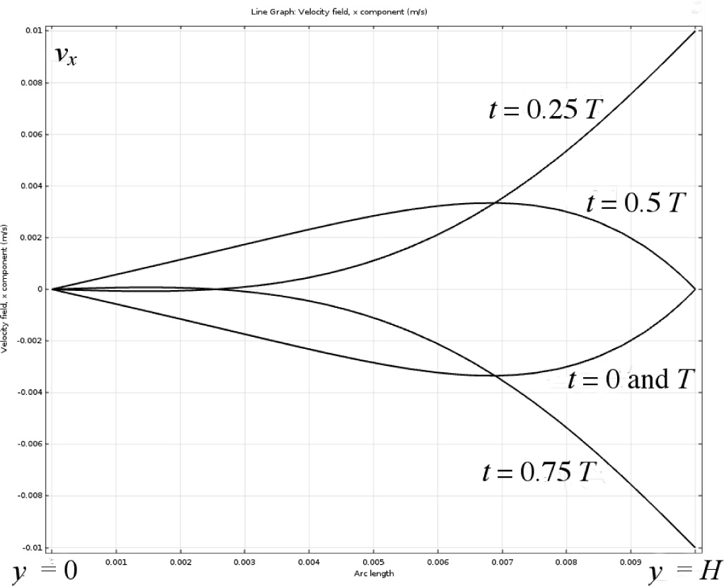
Fig. E6.4.3. Plot of vx (m/s) against distance y (m), for one complete cycle of the upper plate. Viscosity μ =0.1 P.
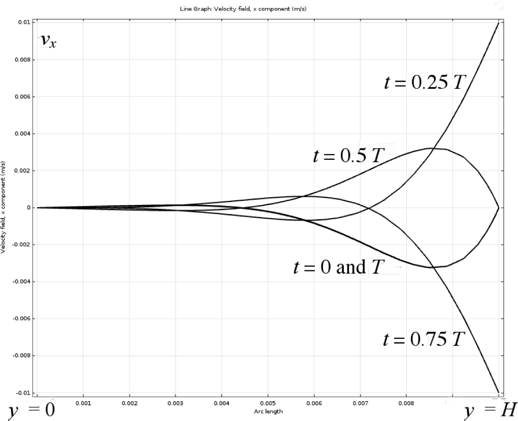
Fig. E6.4.4. Plot of vx (m/s) against distance y (m), for one complete cycle of the upper plate. Viscosity μ =0.5 P.
22. Update the requested times by selecting 1D Plot Group 3. In the Settings window, change the Time selections to t = 19, 19.25, 19.5, 19.75, and 20 s by L-clicking the first value 19 and concluding the selection with Shift + L-click on the value 20, giving five values altogether. L-click Plot.
23. Save the model, in Ex6.4-23.mph for example.
24. Use Step 3 to update the value of mu1 to 0.5 [g/cm/s].
25. R-click the Study node and select Compute.
26. L-click on the 1D Plot Group 3, observe the changes to the solution, and make a final file save.
Discussion of Case 2 (Oscillating Upper-Plate Velocity)
The results for the two values of the viscosity are shown in Figs. E6.4.3 and E6.4.4. Since ω = 2π, the period of the oscillations is T = 1 s. Thus, velocity profiles separated by 0.25 s will occur over one complete cycle of times t = 0, 0.25T , 0.5T , 0.75T , and T . Note two main effects:
(a) Penetration depth. For the lower viscosity, μ =0.1 P, the surface oscillations do not penetrate as far into the liquid as those for the higher viscosity of μ = 0.5 P. In other words, the lower viscosity does not permit as rapid a diffusion of x-momentum as the higher viscosity.
(b) Phase change. Note that for t = T , when the upper plate has a zero velocity, much of the liquid has a negative velocity, largely due to the diffusional effects of the negative surface velocity at an earlier time such as t =0.75T . Similar observations can be made for other values of time.
Both effects have applications in the testing of non-Newtonian fluids, for which the phase difference between stress and strain is illustrated in terms of displacements in Fig. 11.11. Since the velocity vx is the derivative of the distance moved, the displacement D of the upper plate is:
For an infinitely deep liquid, there is again an exact solution:
in which z is the depth and:
The attenuation and phase change with depth z are very apparent from Eqn. (E6.4.4).
6.4 Poiseuille and Couette Flows in Polymer Processing
The study of polymer processing falls into the realm of the chemical engineer. First, the polymer, such as nylon, polystyrene, or polyethylene, is produced by a chemical reaction—either as a liquid or solid. (In the latter event, it would subsequently have to be melted in order to be processed further.) Second, the polymer must be formed by suitable equipment into the desired final shape, such as a film, fiber, bottle, or other molded object. The procedures listed in Table 6.1 are typical of those occurring in polymer processing.
Table 6.1. Typical Polymer-Processing Operations
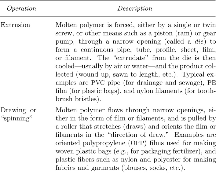
Since polymers are generally highly viscous, their flows can be obtained by solving the equations of viscous motion. In this chapter, we cover the rudiments of extrusion, die flow, and drawing or spinning. The analysis of calendering and coating is considerably more complicated, but can be rendered tractable if reasonable simplifications, known collectively as the lubrication approximation, are made, as discussed in Chapter 8. The treatments of injection molding and blow molding are beyond the scope of this book.
Because molten polymers are usually very viscous, they often need very high pressures to push them through dies. One such “pump” for achieving this is the screw extruder, shown in Fig. E6.5.1. The polymer enters the feed hopper as pellets, falls into the screw channels in the feed section, and is pushed forward by the screw, which rotates at an angular velocity ω, clockwise as seen by an observer looking along the axis from the inlet to the exit (notice that the screw is left-handed). The heated barrel, together with shear effects, melts the pellets, which then become fluid prior to entering the metering section.
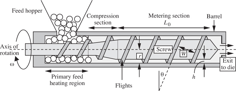
There are three zones in the extruder:
1. In the feed zone the granules are transported into the barrel, where they melt just before entering the compression zone. The large constant depth of the channel in the feed zone means that there will be negligible pressure exerted on the downstream melt in the metering zone.
2. In the compression or “transition” zone the channel depth decreases from the feed zone to the metering zone. Therefore, the melt will gradually increase in pressure as it travels along the compression zone, reaching a maximum pressure at the beginning of the metering zone.
3. In the metering zone, length L0, the screw channel has a constant shallow depth h (with h r) and the melt in the channel should now be homogeneous or uniform. Thus, the metering zone of the screw acts like a constant-delivery pump since the screw is rotating at a constant speed. The melt pressure uniformly increases as it passes along the metering zone. Therefore, calculations of extruder output are based on the metering zone of the screw. Extruder output calculations are relatively simple due to the uniformity of conditions existing in the metering zone of the screw.
The preliminary analysis given here neglects any heat-transfer effects in the metering section, and also assumes that the polymer has a constant Newtonian viscosity μ.
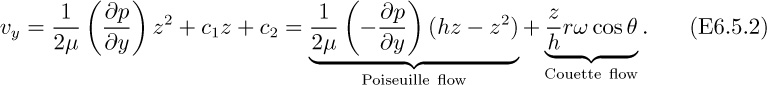
The investigation is facilitated by taking the viewpoint of a hypothetical observer located on the screw, in which case the screw surface and the flights appear to be stationary, with the barrel moving with velocity V = rω at a helix angle θ to the flight axis, as shown in Fig. E6.5.2. The alternative viewpoint of an observer located on the inside surface of the barrel is not very fruitful, because not only are the flights seen as moving boundaries, but the observations would be periodically blocked as the flights passed over the observer! The width of the screw channel measured perpendicularly to the vertical sides of the flight flanks is designated W .
Fig. E6.5.2. Diagonal motion of barrel relative to flights.

Solution
Motion in two principal directions is considered:
1. Flow parallel to the flight axis, caused by a barrel velocity of Vy = V cos θ = rω cos θ relative to the (now effectively stationary) flights and screw.
2. Flow normal to the flight axis, caused by a barrel velocity of Vx = −V sin θ = −rω sin θ relative to the (stationary) flights and screw.
In each case, the flow is considered one-dimensional, with “end-effects” caused by the presence of the flights being unimportant. A glance at Fig. E6.5.3(b) will give the general idea. Although the flow in the x-direction must reverse itself as it nears the flights, it is reasonable to assume for h W that there is a substantial central region in which the flow is essentially in the positive or negative x direction.
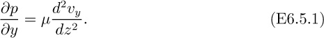
1. Motion parallel to the flight axis. The reader may wish to investigate the additional simplifying assumptions that give the y momentum balance as:
Integration twice yields the velocity profile as:
Here, the integration constants c1 and c2 have been determined in the usual way by applying the boundary conditions:
Note that the negative of the pressure gradient is given in terms of the inlet pressure p1, the exit pressure p2, and the total length L (= L0/ sin θ) measured along the screw flight axis by:

and is a negative quantity since the screw action builds up pressure and p2 >p1. Thus, Eqn. (E6.5.2) predicts a Poiseuille-type backflow (caused by the adverse pressure gradient) and a Couette-type forward flow (caused by the relative motion of the barrel to the screw). The combination is shown in Fig. E6.5.3(a).
Fig. E6.5.3. Fluid motion (a) along, and (b) normal to the flight axis, as seen by an observer on the screw.
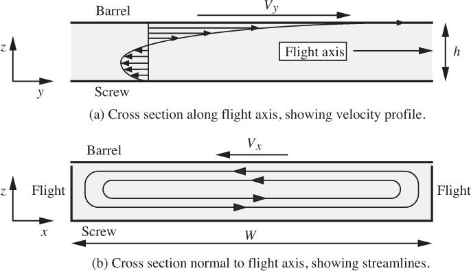
The total flow rate Qy of polymer melt in the direction of the flight axis is obtained by integrating the velocity between the screw and barrel, and recognizing that the width between flights is W :
The actual value of Qy will depend on the resistance of the die located at the extruder exit. In a hypothetical case, in which the die offers no resistance, there would be no pressure increase in the extruder (p2 = p1), leaving only the Couette term in Eqn. (E6.5.5). For the practical situation in which the die offers significant resistance, the Poiseuille term would serve to diminish the flow rate given by the Couette term.
2. Motion normal to the flight axis. By a development very similar to that for flow parallel to the flight axis, we obtain:


Here, Qx is the flow rate in the x direction, per unit depth along the flight axis, and must equal zero, because the flights at either end of the path act as barriers. The negative of the pressure gradient is therefore:
Note from Eqn. (E6.5.10) that vx is zero when either z = 0 (on the screw surface) or z/h =2/3. The reader may wish to sketch the general appearance of vz(z).
Representative values
A COMSOL example follows shortly, and it is appropriate to consider typical measurements and polymer properties for screw extruders2:
2 I heartily thank Mr. John W. Ellis, who is an expert in polymer processing, for supplying these values and most of the information in Table 6.1. Mr. Ellis was previously a faculty member at the Petroleum and Petrochemical College at Chulalongkorn University in Bangkok. He is now R&D Manager at Labtech Engineering Co., Ltd, in Thailand, a company that makes laboratory-size processing machines for the plastics and rubber industries. Mr. Ellis wrote Polymer Products: Design, Materials and Processing, with co-author David Morton-Jones (Chapman and Hall, 1986). His latest book, Introduction to Plastic Foams, co-authored by Dr. Duanghathai Pentrakoon (of the Faculty of Science, Chulalongkorn University, Bangkok), was published by the Chulalongkorn University Press (2005).
1. The size of the screw varies from a laboratory diameter of 20 mm up to large production machines having diameters of 150 mm (very common) or much larger—up to 600 mm.
2. The helix angle is almost always θ = tan−1(1/π)=17.66°, corresponding to a “square thread” screw profile in which the pitch P equals the outside diameter D =2r of the screw.
3. For a 100-mm-diameter screw, a typical channel depth (metering section) would be about h = 5 or 6 mm.
4. The screw rpm ranges from a slow speed of about 30 rpm to a high speed of 150 rpm. The large extruders run at a slower rpm. A typical screw surface speed (the barrel velocity relative to the screw) for extruding polyethylene is 0.5 m/s. For a 100-mm screw, a typical screw speed would be 65 rpm.
5. The metering section length L0 depends on the type of polymer being used— amorphous, semicrystalline, etc. This length is usually expressed as a multiple of the screw diameter, such as L0 = 6.5D. Typical extruder screws have an overall length of 25D.
6. Polymers generally “shear thin” with increasing shear rate, so the viscosity will depend on the prevailing shear rate (related to rpm) of the melt in the screw channel at the melt temperature being used. But for extrusion processes we can assume a melt viscosity of anything between 200 and 1,000 N s/m2 (i.e., Pa s) for extrusion grades of polyolefins (LDPE, HDPE, and PP).
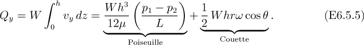
Fig. E6.6.1. Cross-section of the screw extruder normal to the flight axis. The types of boundary conditions are indicated. The pressure is specified to be zero at the midpoint B of the bottom wall. Eventually, a velocity cross-plot will be made between midpoints A and B of the top and bottom surfaces. The transverse coordinate has been changed from z to y to conform to the COMSOL convention.
Consider the screw extruder just discussed in Example 6.5. Solve the equations of motion to determine as precisely as possible the flow pattern given approximately in Fig. E6.5.3(b), normal to the flight axis. Note that the pressure cannot be allowed to “float”, but must be specified to some arbitrary value at any one point in the cross section shown in Fig. E6.6.1, such as the midpoint B.
Based on the comments at the end of Example 6.5, use the following values, which relate to the extrusion of a polyolefin:
1. Polymer properties: ρ = 800 kg/m3, μ = 500 Pa s (N s/m2).
2. Rotational speed N = 65 rpm, so that ω =2π × 65/60 = 6.8 rad/s.
3. Channel depth h = 5 mm = 0.005 m.
4. For a square pitch, the pitch P and screw diameter D are identical, taken to be 100 mm = 0.1 m. The distance between flights is W = P cos θ = 0.1 × cos 17.66° =0.0953 m. For simplicity in our example, we shall round up slightly and take W =0.1 m.
5. The relative velocity is V = ωr = ωD/2 = 6.8 × 0.1/2 = 0.340 m/s, with x component Vx = −0.340 × sin θ = −0.340 × sin 17.66° = −0.103 . = −0.1 m/s.
6. After solving for the flow pattern, make the following plots:
(a) A picture that shows 10 streamlines, one with the true aspect ratio and another with the y-axis “stretched” by a factor of five.
(b) An arrow plot of the x-velocities.
(c) A contour plot of the pressure distribution.
(d) A cross-section plot of the x-velocity between the midpoints A (0.05, 0.005) of the upper moving surface and B (0.05, 0) of the lower stationary surface.
Solution
See Chapter 14 for more details about COMSOL Multiphysics. All mouse-clicks are left-clicks (the same as Select) unless specifically denoted as right-click (R).
Select the Physics
1. Select Model Wizard, 2D, Fluid Flow (the little rotating triangle is called a “glyph”), Single-Phase Flow, Laminar Flow. Add. Note COMSOL’s symbols for pressure and velocity. Study, Stationary, Done.
Define the Parameters
2. R-Global Definitions, Parameters. Enter rho1 = 800 [kg/m3], mu1 = 500 [Pa*s], Vx = −0.1 [m/s] under the Name/Expression columns. (The names rho and mu are reserved by COMSOL for its own use, and so are unavailable to us.)
Establish the Geometry
3. R-Geometry, Rectangle. Note Corner is at x = 0, y = 0. Width = 0.1, Height = 0.005. Build Selected. R-Geometry, Point (this is where we shall specify p = 0). Enter 0.05 and 0.00 for x and y. Build Selected.
Define the Fluid Properties
4. Under Component1, R-Materials, Blank Material. Enter rho1 and mu1 as values. To see the equations being solved, R-click Laminar Flow and select the Equations glyph in the Settings window.
Define the Boundary Conditions
5. R-Laminar Flow, Wall, Wall 2. Hover over the top wall (turns red), L-click to select. Boundary Condition, Sliding Wall. Enter Vx for Uw. Set pressure constraint with R-Laminar Flow, Points, Pressure Point Constraint. Hover over bottom center point and select with L-click (note Pressure is zero). Point 1 should appear in the Active Window.
Create the Mesh and Solve the Problem
6. Mesh 1, Element size, Coarse, Build All. R-Mesh 1, Statistics and note 14,695 elements. To see some of the elements, use the Zoom icon three items, then Zoom Extents to revert.
7. R-Study, Compute (takes about 4 seconds). Gives velocity magnitude, not of interest here.
Display the Streamlines
8. R-Results, 2D Plot Group. R-2D Plot Group 3, Streamline. Settings window, Positioning, Start point controlled, 20 points, yields Fig. E6.6.2.
Fig. E6.6.2. Streamlines, in which the aspect ratio is the same as in the problem statement. The two arrows have been added to emphasize the counter-clockwise direction of flow.
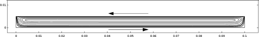
Fig. E6.6.3. Streamlines, in which the height, from y = 0 to 0.005 m has been “stretched” to show more detail. The two arrows have been added to emphasize the counter-clockwise direction of flow.

9. Stretch the y-axis to improve visibility by R-Definitions (under Component 1), View. L-click the glyph at the left of View 2 to expand its tree, Axis. Settings, View Scale, Manual, y-scale factor = 5, Update, Zoom Extents. Streamline 1 then gives Fig. E6.6.3.
Display the Arrow Velocity Plot
10. View 1. R-click Results, 2D Plot Group. R-click 2D Plot Group 4, Arrow Surface 1. Plot. Scale Factor, move slider to right to give Scale Factor 0.034, Color black.
11. In the Graphics window, zoom in and out by either: (a) simultaneously holding the middle mouse button down and moving the mouse forwards and backwards, or (b) clicking on Zoom above the Graphics window and holding the R mouse button down to move the graphics around, giving Fig. E6.6.4.
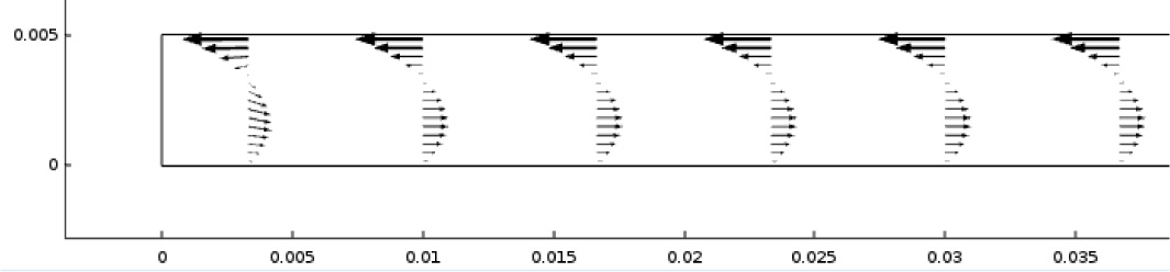
Fig. E6.6.4. Arrow plot, in which the arrow length is proportional to the local velocity. To improve legibility, only the left portion has been reproduced and enlarged.
Display the Isobars
12. R-click Results and L-click 2D Plot Group.
13. L-click the dropbox (under Definitions for Component 1) for View and select View 1.
14. R-click the new 2D Plot Group 5 and L-click Contour.
Fig. E6.6.5. Isobars, with the pressure p = 0 at the midpoint, varying from p . = −5.9 × 10⁵ Pa at the midpoint of the right-hand end to p = 5.9 × 10⁵ Pa at the left-hand end. Note that except for the two upper corners, where there is a conflict in velocities between the moving and no-slip boundaries, the pressure depends only on the horizontal coordinate x.

15. In Settings, Expression field, enter pressure, p. Levels field, change the Entry Method from Number of Levels to Levels. In the Levels field, enter the pressure range as range(−0.6e6, 0.1e6, 0.6e6), Plot; “range” is a function whose first and last parameters denote the start and end; the middle parameter is the increment.
16. By comparing the isobars with the color bar, or by selecting Level Labels, note that the pressure varies from approximately −5.9 × 10⁵ Pa at the midpoint of the right end to approximately 5.9 × 10⁵ Pa at the midpoint of the left end, and zero in the middle.
17. Change Coloring to Uniform and the Color to black to generate Fig. E6.6.5.
Construct the Velocity Cross-Plot
18. Section the data set at the midpoint in the y-direction: R-click Data Sets within the Results tree and select Cut Line 2D. In the Settings window enter (0.05, 0) and (0.05, 0.005) for Points 1 and 2. L-click Plot to display the cut line.
19. R-click Results and L-click 1D Plot Group 6. In the Settings window, L-click the dropdown dialog and change the data set to Cut Line 2D 1.
20. R-click the 1D Plot Group 6 and select Line Graph 1.
21. Within Settings, Expression field, enter u, the x-velocity component. Expand the Coloring and Style section by L-clicking the triangular glyph at the left.
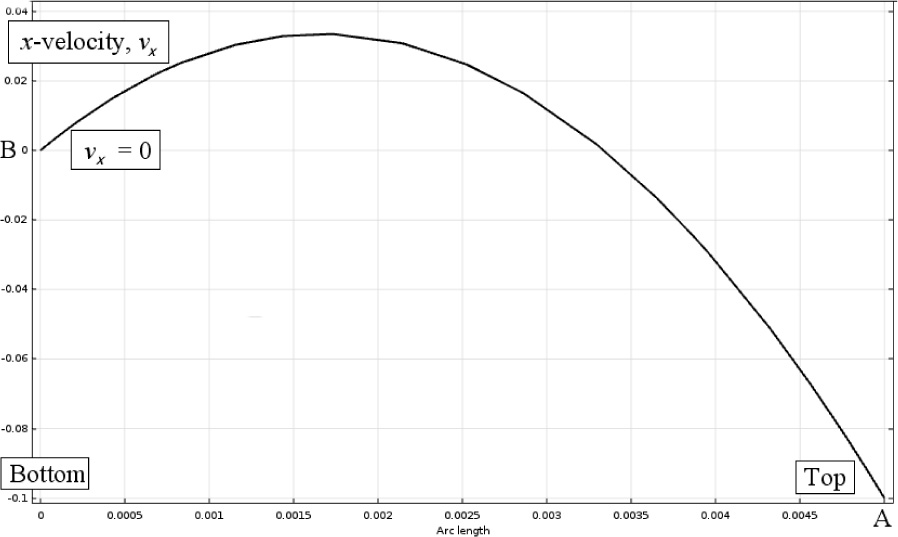
Fig. E6.6.6. A cross-plot that shows how the horizontal velocity vx varies from the midpoint A of the top surface, where it is strongly negative, to the midpoint B of the bottom surface, where it is zero.
22. Change the Color option to Black by L-clicking the dropdown dialog box.
23. L-click Plot at the top of the Settings window to update the plot. There is a Recovery option at the bottom of the Settings window under the Quality section. Select Recover Within Domains, which does polynomial smoothing, giving Fig. E6.6.6.
Discussion of Results
The COMSOL results are shown in Figs. E6.6.2–E6.6.6. The arrow plot of Fig. E6.6.4 clearly shows that the velocity profile is virtually unchanged over the whole width of the cross-section. Near the top surface the flow is induced by the moving surface to be in the negative x-direction. Towards the fixed bottom surface there is a flow reversal, so that at any value of x the net flow rate ![]() is zero.
is zero.
Fig. E6.6.2, which contains 20 streamlines, now indicates that the essential flow reversal occurs very close to each end of the cross-section. To make the flow pattern more clear, the streamlines are repeated in Fig. E6.6.3, in which a larger scale is employed in the y-direction—that is, the x/y geometry is no longer to scale.
The pressure distribution is shown in Fig. E6.6.5 as a series of isobars. Note that the isobars are spaced very evenly, and that the pressure increase from right to left (at the end mid-points) is from −5.9 × 10⁵ Pa to 5.9 × 10⁵ Pa, or 1.18 × 10⁶ Pa total.
Recall that the simplified theory gave the pressure gradient as:
Thus, the theoretical increase in pressure from right to left should be:

in complete agreement with the more accurate two-dimensional solution of the Navier-Stokes equations shown in Fig. E6.6.5.
Finally, Fig. E6.6.6 shows how vx varies from the midpoint A of the top surface to the midpoint B of the bottom surface. As explained in Eqn. E6.5.7, there are two contributions to this velocity profile:
1. A Couette flow from right to left, driven by the leftward-moving top surface.
2. A Poiseuille flow from left to right, driven by the excess pressure at the left.
6.5 Solution of the Equations of Motion in Cylindrical Coordinates
Several chemical engineering operations exhibit symmetry about an axis z and involve one or more surfaces that can be described by having a constant radius for a given value of z. Examples are flow in pipes, extrusion of fibers, and viscometers that involve flow between concentric cylinders, one of which is rotating. Such cases lend themselves naturally to solution in cylindrical coordinates, and two examples will now be given.
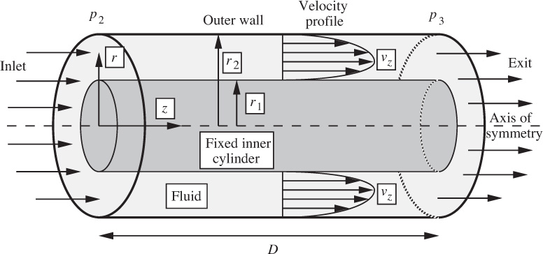
Following the discussion of polymer processing in the previous section, now consider flow through a die that could be located at the exit of the screw extruder of Example 6.6. Consider a die that forms a tube of polymer (other shapes being sheets and filaments). In the die of length D shown in Fig. E6.7, a pressure difference p2 − p3 causes a liquid of viscosity μ to flow steadily from left to right in the annular area between two fixed concentric cylinders. Note that p2 is chosen for the inlet pressure in order to correspond to the extruder exit pressure from Example 6.5. The inner cylinder is solid, whereas the outer one is hollow; their radii are r1 and r2, respectively. The problem, which could occur in the extrusion of plastic tubes, is to find the velocity profile in the annular space and the total volumetric flow rate Q. Note that cylindrical coordinates are now involved.
Fig. E6.7. Geometry for flow through an annular die.
Assumptions and continuity equation
The following assumptions are realistic:
1. There is only one nonzero velocity component, namely that in the direction of flow, vz. Thus, vr = vθ =0.
2. Gravity acts vertically downward, so that gz =0.
3. The axial velocity is independent of the angular location; that is, ∂vz/∂θ =0. To analyze the situation, again start from the continuity equation, (5.49):
which, for constant density and vr = vθ = 0, reduces to:
verifying that vz is independent of distance from the inlet, and that the velocity profile vz = vz(r) appears the same for all values of z.
Momentum balances
There are again three momentum balances, one for each of the r, θ, and z directions. If explored, the first two of these would ultimately lead to the pressure variation with r and θ at any cross section, which is of little interest in this problem. Therefore, we extract from Eqn. (5.75) only the z momentum balance:

With vr = vθ = 0 (from assumption 1), ∂vz/∂z = 0 [from Eqn. (E6.7.1)], ∂vz/∂θ = 0 (assumption 3), and gz = 0 (assumption 2), this momentum balance simplifies to:

in which total derivatives are used because vz depends only on r.
Shortly, we shall prove that the pressure gradient is uniform between the die inlet and exit, being given by:
in which both sides of the equation are positive quantities. Two successive integrations of Eqn. (E6.7.3) may then be performed, yielding:

The two constants may be evaluated by applying the boundary conditions of zero velocity at the inner and outer walls,
giving:

Substitution of these values for the constants of integration into Eqn. (E6.7.5) yields the final expression for the velocity profile:

which is sketched in Fig. E6.7. Note that the maximum velocity occurs somewhat before the halfway point in progressing from the inner cylinder to the outer cylinder.
Volumetric flow rate
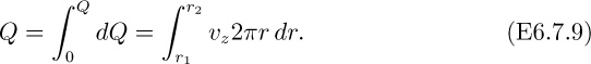
The final quantity of interest is the volumetric flow rate Q. Observing first that the flow rate through an annulus of internal radius r and external radius r + dr is dQ = vz2πr dr, integration yields:
Since r ln r is involved in the expression for vz, the following indefinite integral is needed:

giving the final result:

Since Q, μ, r1, and r2 are constant throughout the die, ∂p/∂z is also constant, thus verifying the hypothesis previously made. Observe that in the limiting case of r1 → 0, Eqn. (E6.7.11) simplifies to the Hagen-Poiseuille law, already stated in Eqn. (3.12).
This problem may also be solved by performing a momentum balance on a shell that consists of an annulus of internal radius r, external radius r + dr, and length dz.
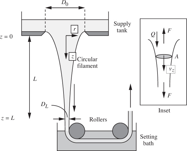
A Newtonian polymeric liquid of viscosity μ is being “spun” (drawn into a fiber or filament of small diameter before solidifying by pulling it through a chemical setting bath) in the apparatus shown in Fig. E6.8.
The liquid volumetric flow rate is Q, and the filament diameters at z = 0 and z = L are D0 and DL, respectively. To a first approximation, neglect the effects of gravity, inertia, and surface tension (this last effect is examined in detail in Problem 6.26). Derive an expression for the tensile force F needed to pull the filament downward. Assume that the axial velocity profile is “flat” at any vertical location, so that vz depends only on z, which is here most conveniently taken as positive in the downward direction. Also derive an expression for the downward velocity vz as a function of z. The inset of Fig. E6.8 shows further details of the notation concerning the filament.
Fig. E6.8. “Spinning” a polymer filament, whose diameter in relation to its length is exaggerated in the diagram.
Solution
It is first necessary to determine the radial velocity and hence the pressure inside the filament. From continuity: 1 r

Since vz depends only on z, its axial derivative is a function of z only, or dvz/dz = f(z), so that Eqn. (E6.8.1) may be rearranged and integrated at constant z to give:
(E6.8.2) But to avoid an infinite value of vr at the centerline, g(z) must be zero, giving:
To proceed with reasonable expediency, it is necessary to make some simplification. After accounting for a primary effect (the difference between the pressure in the filament and the surrounding atmosphere), we assume that a secondary effect (variation of pressure across the filament) is negligible; that is, the pressure does not depend on the radial location (see Problem 6.27 for a more accurate investigation). Note that the external (gauge) pressure is zero everywhere, and apply the first part of Eqn. (5.64) at the free surface:
The axial stress is therefore:
It is interesting to note that the same result can be obtained with an alternative assumption.3 The axial tension in the fiber equals the product of the cross-sectional area and the local axial stress:
3 See S. Middleman’s Fundamentals of Polymer Processing, McGraw-Hill, New York, 1977, p. 235. There, the author assumes σrr = σθθ = 0, followed by the identity: p = −(σzz + σrr + σθθ)/3.
Since the effect of gravity is stated to be insignificant, F is a constant, regardless of the vertical location.
At any location, the volumetric flow rate equals the product of the cross-sectional area and the axial velocity:
A differential equation for the velocity is next obtained by dividing one of the last two equations by the other, and rearranging: 1 vz

Integration, noting that the inlet velocity at z =0 is ![]() gives:
gives:

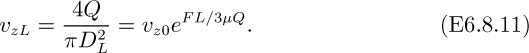
so that the axial velocity increases exponentially with distance:
The tension is obtained by applying Eqns. (E6.8.7) and (E6.8.10) just before the filament is taken up by the rollers:
Rearrangement yields:
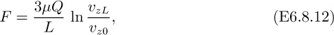
which predicts a force that increases with higher viscosities, flow rates, and draw-down ratios (vzL/vz0), and that decreases with longer filaments.
Elimination of F from Eqns. (E6.8.10) and (E6.8.12) gives an expression for the velocity that depends only on the variables specified originally:
(E6.8.13)
a result that is independent of the viscosity.
6.6 Solution of the Equations of Motion in Spherical Coordinates
Most of the introductory viscous-flow problems will lend themselves to solution in either rectangular or cylindrical coordinates. Occasionally, as in Example 6.7, a problem will arise in which spherical coordinates should be used. It is a fairly advanced problem! Try first to appreciate the broad steps involved, and then peruse the fine detail at a second reading.
The problem concerns the analysis of a cone-and-plate rheometer, an instrument developed and perfected in the 1950s and 1960s by Prof. Karl Weissenberg, for measuring the viscosity of liquids, and also known as the “Weissenberg rheogoniometer.”4 A cross section of the essential features is shown in Fig. E6.9, in which the liquid sample is held by surface tension in the narrow opening between a rotating lower circular plate, of radius R, and an upper cone, making an angle of β with the vertical axis. The plate is rotated steadily in the ϕ direction with an angular velocity ω, causing the liquid in the gap to move in concentric circles with a velocity vϕ. (In practice, the tip of the cone is slightly truncated, to avoid friction with the plate.) Observe that the flow is of the Couette type.
4 Professor Weissenberg (1893–1976) once related to the author that he (Prof. Weissenberg) was attending an instrument trade show in London. There, the rheogoniometer was being demonstrated by a young salesman who was unaware of Prof. Weissenberg’s identity. Upon inquiring how the instrument worked, the salesman replied: “I’m sorry, sir, but it’s quite complicated, and I don’t think you will be able to understand it.”
Fig. E6.9. Geometry for a Weissenberg rheogoniometer. (The angle between the cone and plate is exaggerated.)

The top of the upper shaft—which acts like a torsion bar—is clamped rigidly. However, viscous friction will twist the cone and the lower portions of the upper shaft very slightly; the amount of motion can be detected by a light arm at the extremity of which is a transducer, consisting of a small piece of steel, attached to the arm, and surrounded by a coil of wire; by monitoring the inductance of the coil, the small angle of twist can be obtained; a knowledge of the elastic properties of the shaft then enables the restraining torque T to be obtained. From the analysis given below, it is then possible to deduce the viscosity of the sample. The instrument is so sensitive that if no liquid is present, it is capable of determining the viscosity of the air in the gap!
The problem is best solved using spherical coordinates, because the surfaces of the cone and plate are then described by constant values of the angle θ, namely β and π/2, respectively.
Assumptions and the continuity equation
The following realistic assumptions are made:
1. There is only one nonzero velocity component, namely that in the ϕ direction, vϕ. Thus, vr = vθ =0.
2. Gravity acts vertically downward, so that gϕ =0.
3. We do not need to know how the pressure varies in the liquid. Therefore, the r and θ momentum balances, which would supply this information, are not required.
The analysis starts once more from the continuity equation, (5.50):

which, for constant density and vr = vθ = 0 reduces to:
verifying that vϕ is independent of the angular location ϕ, so we are correct in examining just one representative cross section, as shown in Fig. E6.9.
Momentum balances
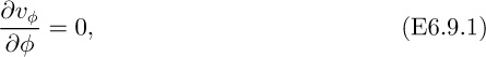
There are again three momentum balances, one for each of the r, θ, and ϕ directions. From the third assumption above, the first two such balances are of no significant interest, leaving, from Eqn. (5.77), just that in the ϕ direction:
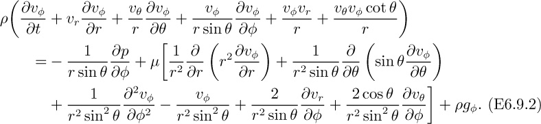
With vr = vθ = 0 (assumption 1), ∂vϕ/∂ϕ = 0 [from Eqn. (E6.9.1)], and gϕ = 0 (assumption 2), the momentum balance simplifies to:

Determination of the velocity profile
First, seek an expression for the velocity in the ϕ direction, which is expected to be proportional to both the distance r from the origin and the angular velocity ω of the lower plate. However, its variation with the coordinate θ is something that has to be discovered. Therefore, postulate a solution of the form:
in which the function f(θ) is to be determined. Substitution of vϕ from Eqn. (E6.9.4) into Eqn. (E6.9.3), and using f and f to denote the first and second total derivatives of f with respect to θ, gives:
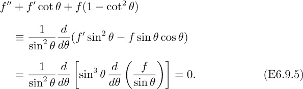
The reader is encouraged, as always, to check the missing algebraic and trigonometric steps, although they are rather tricky here!5
5 Although our approach is significantly different from that given on page 98 et seq. of R.B. Bird, W.E. Stewart, and E.N. Lightfoot, Transport Phenomena, Wiley & Sons, New York, 1960, we are indebted to these authors for the helpful hint they gave in establishing the equivalency expressed in our Eqn. (E6.9.5).
By multiplying Eqn. (E6.9.5) through by sin2 θ, it follows after integration that the quantity in brackets is a constant, here represented as −2c1, the reason for the “−2” being that it will cancel with a similar factor later on:
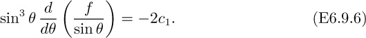
Separation of variables and indefinite integration (without specified limits) yields:

To proceed further, we need the following two standard indefinite integrals and one trigonometric identity6:
6 From pages 87 (integrals) and 72 (trigonometric identity) of J.H. Perry, ed., chemical Engineers’ Handbook,


Armed with these, Eqn. (E6.9.7) leads to the following expression for f:

in which c2 is a second constant of integration.
Implementation of the boundary conditions
The constants c1 and c2 are found by imposing the two boundary conditions:
1. At the lower plate, where θ = π/2 and the expression in parentheses in Eqn. (E6.9.11) is zero, so that f = c2, the velocity is simply the radius times the angular velocity:
2. At the surface of the cone, where θ = β, the velocity vϕ = rωf is zero. Hence f = 0, and Eqn. (E6.9.11) leads to:

Substitution of these expressions for c1 and c2 into Eqn. (E6.9.11), and noting that vϕ = rωf, gives the final (!) expression for the velocity:
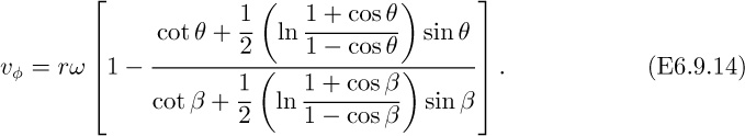
As a partial check on the result, note that Eqn. (E6.9.14) reduces to vϕ = rω when θ = π/2 and to vϕ = 0 when θ = β.
Shear stress and torque
Recall that the primary goal of this investigation is to determine the torque T needed to hold the cone stationary. The relevant shear stress exerted by the liquid on the surface of the cone is τθϕ—that exerted on the under surface of the cone (of constant first subscript, θ = β) in the positive ϕ direction (refer again to Fig. 5.12 for the sign convention and notation for stresses). Since this direction is the same as that of the rotation of the lower plate, we expect that τθϕ will prove to be positive, thus indicating that the liquid is trying to turn the cone in the same direction in which the lower plate is rotated.
From the second of Eqn. (5.65), the relation for this shear stress is:

Since vθ = 0, and recalling Eqns. (E6.9.4), (E6.9.6), and (E6.9.13), the shear stress on the cone becomes:

One importance of this result is that it is independent of r, giving a constant stress and strain throughout the liquid, a significant simplification when deciphering the experimental results for non-Newtonian fluids (see Chapter 11). In effect, the increased velocity differences between the plate and cone at the greater values of r are offset in exact proportion by the larger distances separating them.
The torque exerted by the liquid on the cone (in the positive ϕ direction) is obtained as follows. The surface area of the cone between radii r and r + dr is 2πr sin βdr, and is located at a lever arm of r sin β from the axis of symmetry. Multiplication by the shear stress and integration gives:
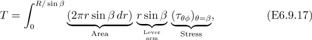
Substitution of (τθϕ)θ=β from Eqn. (E6.9.16) and integration gives the torque as:
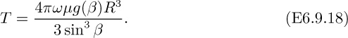
Problem 6.15 reaches essentially the same conclusion much more quickly for the case of a small angle between the cone and the plate. The torque for holding the cone stationary has the same value, but is, of course, in the negative ϕ direction.
Since R and g(β) can be determined from the radius and the angle β of the cone in conjunction with Eqn. (E6.9.13), the viscosity μ of the liquid can finally be determined.
Problems for Chapter 6
Unless otherwise stated, all flows are steady state, for a Newtonian fluid with constant density and viscosity.
1. Stretching of a liquid film—M. In broad terms, explain the meanings of the following two equations, paying attention to any sign convention:
Fig. P6.1. Stretching of liquid film between two bars.
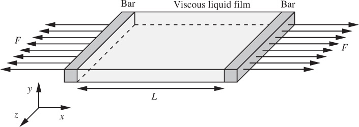
Fig. P6.1 shows a film of a viscous liquid held between two bars spaced a distance L apart. If the film thickness is uniform, and the total volume of liquid is V , show that the force necessary to separate the bars with a relative velocity dL/dt is:
Fig. P6.2. Coating of wire drawn through a die.

2. Wire coating—M. Fig. P6.2 shows a rodlike wire of radius r1 that is being pulled steadily with velocity V through a horizontal die of length L and internal radius r2. The wire and the die are coaxial, and the space between them is filled with a liquid of viscosity μ. The pressure at both ends of the die is atmospheric. The wire is coated with the liquid as it leaves the die, and the thickness of the coating eventually settles down to a uniform value, δ.
Neglecting end effects, use the equations of motion in cylindrical coordinates to derive expressions for:
(a) The velocity profile within the annular space. Assume that there is only one nonzero velocity component, vz, and that this depends only on radial position.
(b) The total volumetric flow rate Q through the annulus.
(c) The limiting value for Q if r1 approaches zero.
(d) The final thickness, δ, of the coating on the wire. (Here, only an equation is needed from which δ could be found.)
(e) The force F needed to pull the wire.
3. Off-center annular flow—D (C). A liquid flows under a pressure gradient ∂p/∂z through the narrow annular space of a die, a cross section of which is shown in Fig. P6.3(a). The coordinate z is in the axial direction, normal to the plane of the diagram. The die consists of a solid inner cylinder with center P and radius b inside a hollow outer cylinder with center O and radius a. The points O and P were intended to coincide, but due to an imperfection of assembly are separated by a small distance δ.
Fig. P6.3. Off-center cylinder inside a die (gap width exaggerated): (a) complete cross section; (b) effect of incrementing θ.
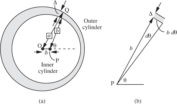
By a simple geometrical argument based on the triangle OPQ, show that the gap width Δ between the two cylinders is given approximately by:
Δ = a − b − δ cos θ,
where the angle θ is defined in the diagram.
Now consider the radius arm b swung through an angle dθ, so that it traces an arc of length bdθ. The flow rate dQ through the shaded element in Fig. P6.3(b) is approximately that between parallel plates of width bdθ and separation Δ. Hence, prove that the flow rate through the die is given approximately by:
Q = πbc(2α3 +3αδ2),
in which:
Assume from Eqn. (E6.1.26) that the flow rate per unit width between two flat plates separated by a distance h is:

What is the ratio of the flow rate if the two cylinders are touching at one point to the flow rate if they are concentric?
4. Compression molding—M. Fig. P6.4 shows the (a) beginning, (b) intermediate, and (c) final stages in the compression molding of a material that behaves as a liquid of high viscosity μ, from an initial cylinder of height H0 and radius R0 to a final disk of height H1 and radius R1.

Fig. P6.4. Compression molding between two disks.
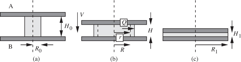
In the molding operation, the upper disk A is squeezed with a uniform velocity V toward the stationary lower disk B.
(a) Derive expressions for H and R as functions of time t, H0, and R0.
(b) Consider the radially outward volumetric flow rate Q per unit perimeter, crossing a cylinder of radius r, as in Fig. P6.4(b). Obtain a relation for Q in terms of V and r.
(c) Assume by analogy from Eqn. (E6.1.26) that per unit width of a channel of depth H, the volumetric flow rate is:
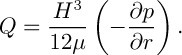
(d) Ignoring small variations of pressure in the z direction, derive an expression for the radial variation of pressure.
(e) Prove that the total compressive force F that must be exerted downward on the upper disk is:
(f) Draw a sketch that shows how F varies with time.
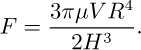
5. Film draining—M. Fig. P6.5 shows an idealized view of a liquid film of viscosity μ that is draining under gravity down the side of a flat vertical wall. Such a situation would be approximated by the film left on the wall of a tank that was suddenly drained through a large hole in its base.
Fig. P6.5. Liquid draining from a vertical wall.
What are the justifications for assuming that the velocity profile at any distance x below the top of the wall is given by:
where h = h(x) is the local film thickness? Derive an expression for the corresponding downward mass flow rate m per unit wall width (normal to the plane of the diagram).
Perform a transient mass balance on a differential element of the film and prove that h varies with time and position according to:

Now substitute your expression for m, to obtain a partial differential equation for h. Try a solution of the form:
h = ctpxq,
and determine the unknowns c, p, and q. Discuss the limitations of your solution.
Note that a similar situation occurs when a substrate is suddenly lifted from a bath of coating fluid.
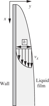
6. Sheet “spinning”—M. A Newtonian polymeric liquid of viscosity μ is being “spun” (drawn into a sheet of small thickness before solidifying by pulling it through a chemical setting bath) in the apparatus shown in Fig. P6.6.
Fig. P6.6. “Spinning” a polymer sheet.
The liquid volumetric flow rate is Q, and the sheet thicknesses at z = 0 and z = L are Δ and δ, respectively. The effects of gravity, inertia, and surface tension are negligible. Derive an expression for the tensile force needed to pull the filament downward. Hint: Start by assuming that the vertically downward velocity vz depends only on z and that the lateral velocity vy is zero. Also derive an expression for the downward velocity vz as a function of z.
7. Details of pipe flow—M. A fluid of density ρ and viscosity μ flows from left to right through the horizontal pipe of radius a and length L shown in Fig. P6.7. The pressures at the centers of the inlet and exit are p1 and p2, respectively. You may assume that the only nonzero velocity component is vz, and that this is not a function of the angular coordinate, θ.
Stating any further necessary assumptions, derive expressions for the following, in terms of any or all of a, L, p1, p2, ρ, μ, and the coordinates r, z, and θ:
(a) The velocity profile, vz = vz(r).
(b) The total volumetric flow rate Q through the pipe.
(c) The pressure p at any point (r, θ, z).
(d) The shear stress, τrz.
Fig. P6.7. Flow of a liquid in a horizontal pipe.

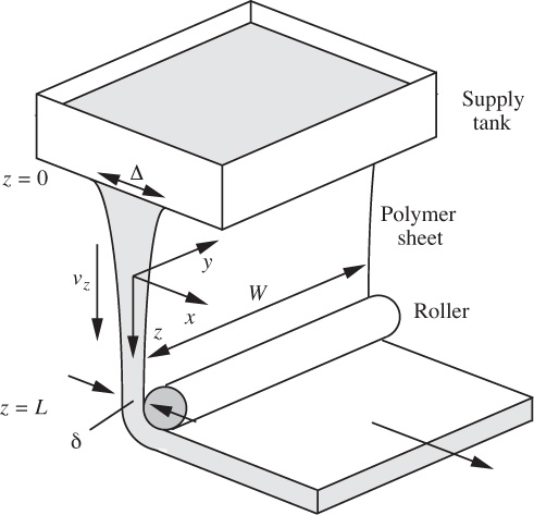
8. Natural convection—M. Fig. P6.8 shows two infinite parallel vertical walls that are separated by a distance 2d. A fluid of viscosity μ and volume coefficient of expansion β fills the intervening space. The two walls are maintained at uniform temperatures T1 (cold) and T2 (hot), and you may assume (to be proved in a heat-transfer course) that there is a linear variation of temperature in the x direction. That is:

Fig. P6.8. Natural convection between vertical walls.
The density is not constant, but varies according to:
where ![]() is the density at the mean temperature
is the density at the mean temperature ![]() , which occurs at x =0.
, which occurs at x =0.
If the resulting natural-convection flow is steady, use the equations of motion to derive an expression for the velocity profile vy = vy(x) between the plates. Your expression for vy should be in terms of any or all of x, d, T1, T2, ![]() , μ, β, and g.
, μ, β, and g.
Hints: In the y momentum balance, you should find yourself facing the following combination:
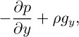
in which gy = −g. These two terms are almost in balance, but not quite, leading to a small—but important—buoyancy effect that “drives” the natural convection. The variation of pressure in the y direction may be taken as the normal hydrostatic variation:

We then have:

and this will be found to be a vital contribution to the y momentum balance.
9. Square duct velocity profile—M. A certain flow in rectangular Cartesian coordinates has only one nonzero velocity component, vz, and this does not vary with z. If there is no body force, write down the Navier-Stokes equation for the z momentum balance.
Fig. P6.9. Square cross section of a duct.

One-dimensional, fully developed steady flow occurs under a pressure gradient ∂p/∂z in the z direction, parallel to the axis of a square duct of side 2a, whose cross section is shown in Fig. P6.9. The following equation has been proposed for the velocity profile:
Without attempting to integrate the momentum balance, investigate the possible merits of this proposed solution for vz. Explain whether or not it is correct.
Fig. P6.10. Square cross section of a duct.
10. Poisson’s equation for a square duct—E. A polymeric fluid of uniform viscosity μ is to be extruded after pumping it through a long duct whose cross section is a square of side 2a, shown in Fig. P6.10. The flow is parallel everywhere to the axis of the duct, which is in the z direction, normal to the plane of the diagram.
If ∂p/∂z, μ, and a are specified, show that the problem of obtaining the axial velocity distribution vz = vz(x, y), amounts to solving Poisson’s equation—of the form ∇2ϕ = f(x, y), where f is specified and ϕ is the unknown. Also note that Poisson’s equation can be solved numerically by the COMSOL computational fluid dynamics program introduced in Chapter 14 (see also Example 7.4)
Fig. P6.11. Proposed velocity profiles for immiscible liquids.
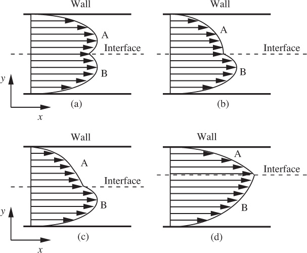
11. Permissible velocity profiles—E. Consider the shear stress τyx; why must it be continuous—in the y direction, for example—and not undergo a sudden step-change in its value? Two immiscible Newtonian liquids A and B are in steady laminar flow between two parallel plates. Which—if any—of the velocity profiles shown in Fig. P6.11 are impossible? Profile A meets the interface normally in (b), but at an angle in (c). Any apparent location of the interface at the centerline is coincidental and should be ignored. Explain your answers carefully.
Fig. P6.12. Viscous flow past a sphere.
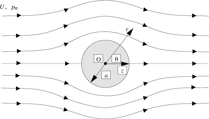
12. “Creeping” flow past a sphere—D. Figure P6.12 shows the steady, “creeping” (very slow) flow of a fluid of viscosity μ past a sphere of radius a. Far away from the sphere, the pressure is p∞ and the undisturbed fluid velocity is U in the positive z direction. The following velocity components and pressure have been proposed in spherical coordinates:
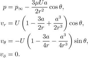
Assuming the velocities are sufficiently small so that terms such as vr(∂vr/∂r) can be neglected, and that gravity is unimportant, prove that these equations do indeed satisfy the following conditions, and therefore are the solution to the problem:
(a) The continuity equation.
(b) The r and θ momentum balances.
(c) A pressure of p∞ and a z velocity of U far away from the sphere.
(d) Zero velocity components on the surface of the sphere.
Also derive an expression for the net force exerted in the z direction by the fluid on the sphere, and compare it with that given by Stokes’ law in Eqn. (4.11).
Note that the problem is one in spherical coordinates, in which the z axis has no formal place, except to serve as a reference direction from which the angle θ is measured. There is also symmetry about this axis, such that any derivatives in the ϕ direction are zero. Note: The actual derivation of these velocities, starting from the equations of motion, is fairly difficult!
Fig. P6.13. Section of a Couette viscometer.
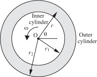
13. Torque in a Couette viscometer—M. Fig. P6.13 shows the horizontal cross section of a concentric cylinder or “Couette” viscometer, which is an apparatus for determining the viscosity μ of the fluid that is placed between the two vertical cylinders. The inner and outer cylinders have radii of r1 and r2, respectively. If the inner cylinder is rotated with a steady angular velocity ω, and the outer cylinder is stationary, derive an expression for vθ (the θ velocity component) as a function of radial location r.
If, further, the torque required to rotate the inner cylinder is found to be T per unit length of the cylinder, derive an expression whereby the unknown viscosity μ can be determined, in terms of T , ω, r1, and r2. Hint: You will need to consider one of the shear stresses given in Table 5.8.
14. Wetted-wall column—M. Fig. P6.14 shows a “wetted-wall” column, in which a thin film of a reacting liquid of viscosity μ flows steadily down a plane wall, possibly for a gas-absorption study. The volumetric flow rate of liquid is specified as Q per unit width of the wall (normal to the plane of the diagram).
Assume that there is only one nonzero velocity component, vx, and that this does not vary in the x direction, and that the gas exerts negligible shear stress on the liquid film. Starting from the equations of motion, derive an expression for the “profile” of the velocity vx (as a function of ρ, μ, g, y, and δ), and also for the film thickness, δ (as a function of ρ, μ, g, and Q).
Fig. P6.14. Wetted-wall column.
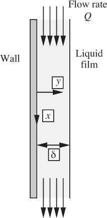
15. Simplified view of a Weissenberg rheogoniometer—M. Consider the Weissenberg rheogoniometer with a very shallow cone; thus, referring to Fig. E6.9, β = π/2 − α, where α is a small angle.
(a) Without going through the complicated analysis presented in Example 6.9, outline your reasons for supposing that the shear stress at any location on the cone is:
(b) Hence, prove that the torque required to hold the cone stationary (or to rotate the lower plate) is:

(c) By substituting β = π/2 − α into Eqn. (E6.9.13) and expanding the various functions in power series (only a very few terms are needed), prove that g(β)= 1/(2α), and that Eqn. (E6.9.18) again leads to the expression just obtained for the torque in part (b) above.
16. Parallel-disk rheometer—M. Fig. P6.16 shows the diametral cross section of a viscometer, which consists of two opposed circular horizontal disks, each of radius R, spaced by a vertical distance H; the intervening gap is filled by a liquid of constant viscosity μ and constant density. The upper disk is stationary, and the lower disk is rotated at a steady angular velocity ω in the θ direction.
Fig. P6.16. Cross section of parallel-disk rheometer.

There is only one nonzero velocity component, vθ, so the liquid everywhere moves in circles. Simplify the general continuity equation in cylindrical coordinates, and hence deduce those coordinates (r?, θ?, z?) on which vθ may depend.
Now consider the θ-momentum equation, and simplify it by eliminating all zero terms. Explain briefly: (a) why you would expect ∂p/∂θ to be zero, and (b) why you cannot neglect the term ∂2vθ/∂z2.
Also explain briefly the logic of supposing that the velocity in the θ direction is of the form vθ = rωf(z), where the function f(z) is yet to be determined. Now substitute this into the simplified θ-momentum balance and determine f(z), using the boundary conditions that vθ is zero on the upper disk and rω on the lower disk.
Why would you designate the shear stress exerted by the liquid on the lower disk as τzθ? Evaluate this stress as a function of radius.
17. Screw extruder optimum angle—M. Note that the flow rate through the die of Example 6.7, given in Eqn. (E6.7.11), can be expressed as:
in which c is a factor that accounts for the geometry.
Suppose that this die is now connected to the exit of the extruder studied in Example 6.5, and that p1 = p3 = 0, both pressures being atmospheric. Derive an expression for the optimum flight angle θopt that will maximize the flow rate Qy through the extruder and die. Give your answer in terms of any or all of c, D, h, L0, r, W , μ, and ω.
For what value of c would the pressure at the exit of the extruder approach its largest possible value p2max? Derive an expression for p2max.
18. Annular flow in a die—E. Referring to Example 6.7, concerning annular flow in a die, answer the following questions, giving your explanation in both cases:
(a) What form does the velocity profile, vz = vz(r), assume as the radius r1 of the inner cylinder becomes vanishingly small?
(b) Does the maximum velocity occur halfway between the inner and outer cylinders, or at some other location?
19. Rotating rod in a fluid—M. Fig. P6.19(a) shows a horizontal cross section of a long vertical cylinder of radius a that is rotated steadily counter-clockwise with an angular velocity ω in a very large volume of liquid of viscosity μ. The liquid extends effectively to infinity, where it may be considered at rest. The axis of the cylinder coincides with the z axis.
Fig. P6.19. Rotating cylinder in (a) a single liquid, and (b) two immiscible liquids.
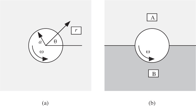
(a) What type of flow is involved? What coordinate system is appropriate?
(b) Write down the differential equation of mass and that one of the three general momentum balances that is most applicable to the determination of the velocity vθ.
(c) Clearly stating your assumptions, simplify the situation so that you obtain an ordinary differential equation with vθ as the dependent variable and r as the independent variable.
(d) Integrate this differential equation, and introduce any boundary condition(s), and prove that vθ = ωa2/r.
(e) Derive an expression for the shear stress τrθ at the surface of the cylinder. Carefully explain the plus or minus sign in this expression.
(f) Derive an expression that gives the torque T needed to rotate the cylinder, per unit length of the cylinder.
(g) Derive an expression for the vorticity component (∇ × v)z. Comment on your result.
(h) Fig. P6.19(b) shows the initial condition of a mixing experiment in which the cylinder is in the middle of two immiscible liquids, A and B, of identical densities and viscosities. After the cylinder has made one complete rotation, draw a diagram that shows a representative location of the interface between A and B.
Fig. P6.20. Two-phase flow between parallel plates.
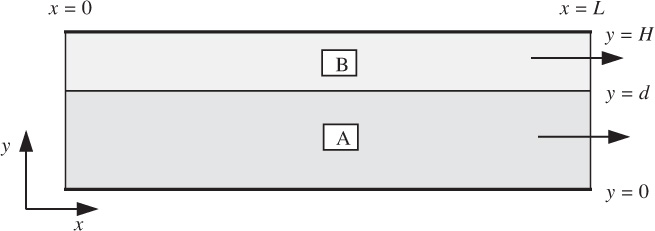
20. Two-phase immiscible flow—M. Fig. P6.20 shows an apparatus for measuring the pressure drop of two immiscible liquids as they flow horizontally between two parallel plates that extend indefinitely normal to the plane of the diagram. The liquids, A and B, have viscosities μA and μB, densities ρA and ρB, and volumetric flow rates QA and QB (per unit depth normal to the plane of the figure), respectively. Gravity may be considered unimportant, so that the pressure is essentially only a function of the horizontal distance, x.
(a) What type of flow is involved?
(b) Considering layer A, start from the differential equations of mass and momentum, and, clearly stating your assumptions, simplify the situation so that you obtain a differential equation that relates the horizontal velocity vxA to the vertical distance y.
(c) Integrate this differential equation so that you obtain vxA in terms of y and any or all of d, dp/dx, μA, ρA, and (assuming the pressure gradient is uniform) two arbitrary constants of integration, say, c1A and c2A. Assume that a similar relationship holds for vxB.
(d) Clearly state the four boundary and interfacial conditions, and hence derive expressions for the four constants, thus giving the velocity profiles in the two layers.
(e) Sketch the velocity profiles and the shear-stress distribution for τyx between the upper and lower plates.
(f) Until now, we have assumed that the interface level y = d is known. In reality, however, it will depend on the relative flow rates QA and QB. Show clearly how this dependency could be obtained, but do not actually carry the analysis through to completion.
Fig. P6.21. Rotating-impeller humidifier.
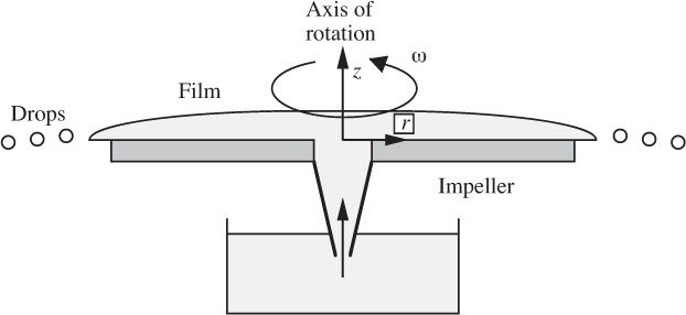
21. Room humidifier—M. Fig. P6.21 shows a room humidifier, in which a circular impeller rotates about its axis with angular velocity ω. A conical extension dips into a water-bath, sucking up the liquid (of density ρ and viscosity μ), which then spreads out over the impeller as a thin laminar film that rotates everywhere with an angular velocity ω, eventually breaking into drops after leaving the periphery.
(a) Assuming incompressible steady flow, with symmetry about the vertical (z) axis, and a relatively small value of vz, what can you say from the continuity equation about the term:

(b) If the pressure in the film is everywhere atmospheric, the only significant inertial term is ![]() , and information from (a) can be used to neglect one particular term, to what two terms does the r momentum balance simplify?
, and information from (a) can be used to neglect one particular term, to what two terms does the r momentum balance simplify?
(c) Hence prove that the velocity vr in the radial direction is a half-parabola in the z direction.
(d) Derive an expression for the total volumetric flow rate Q, and hence prove that the film thickness at any radial location is given by:
where ν is the kinematic viscosity.
Fig. P6.22. Transport of inner cylinder.

22. Transport of inner cylinder—M (C). As shown in Fig. P6.22, a long solid cylinder of radius rc and length L is being transported by a viscous liquid of the same density down a pipe of radius a, which is much smaller than L. The annular gap, of extent a − rc, is much smaller than a. Assume: (a) the cylinder remains concentric within the pipe, (b) the flow in the annular gap is laminar, (c) the shear stress is essentially constant across the gap, and (d) entry and exit effects can be neglected. Prove that the velocity of the cylinder is given fairly accurately by:

where Q is the volumetric flow rate of the liquid upstream and downstream of the cylinder. Hint: Concentrate first on understanding the physical situation. Don’t rush headlong into a lengthy analysis with the Navier-Stokes equations!
Fig. P6.23. Flow between inclined planes.

23. Flow between inclined planes—M (C). A viscous liquid flows between two infinite planes inclined at an angle 2α to each other. Prove that the liquid velocity, which is everywhere parallel to the line of intersection of the planes, is given by:
where z, r, θ are cylindrical coordinates. The z axis is the line of intersection of the planes and the r axis at θ = 0 bisects the angle between the planes. Assume laminar flow, with:
and start by proposing a solution of the form vz = rng(θ)(−∂p/∂z)/μ, where the exponent n and function g(θ) are to be determined.
Fig. P6.24. Flow of two immiscible liquids in a pipe. The thickness Δ of the film next to the wall is exaggerated.
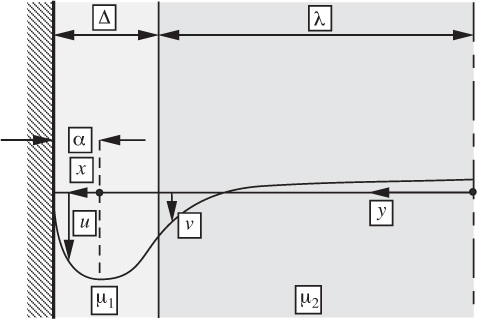
24. Immiscible flow inside a tube—D (C). A film of liquid of viscosity μ1 flows down the inside wall of a circular tube of radius (λ + Δ). The central core is occupied by a second immiscible liquid of viscosity μ2, in which there is no net vertical flow. End effects may be neglected, and steady-state circulation in the core liquid has been reached. If the flow in both liquids is laminar, so that the velocity profiles are parabolic as shown in Fig. P6.24, prove that:

where Δ is the thickness of the liquid film, and α is the distance from the wall to the point of maximum velocity in the film. Fig. P6.24 suggests notation for solving the problem. To save time, assume parabolic velocity profiles without proof: u = a + bx + cx2 and v = d + ey + fy2.
Discuss what happens when λ/Δ → ∞; and also when μ2/μ1 → 0; and when μ1/μ2 → 0.
25. Blowing a polyethylene bubble—D. For an incompressible fluid in cylindrical coordinates, write down:
(a) The continuity equation, and simplify it.
(b) Expressions for the viscous normal stresses σrr and σθθ, in terms of pressure, viscosity, and strain rates.
Fig. P6.25. Cross section of half of a cylindrical bubble.
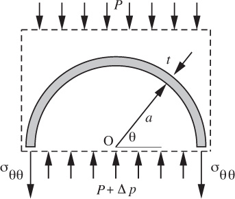
A polyethylene sheet is made by inflating a cylindrical bubble of molten polymer effectively at constant length, a half cross section of which is shown in Fig. P6.25. The excess pressure inside the bubble is small compared with the external pressure P , so that Δp ≪ P and σrr . = −P .
By means of a suitable force balance on the indicated control volume, prove that the circumferential stress is given by σθθ = −P + aΔp/t. Assume pseudo-steady state—that is, the circumferential stress just balances the excess pressure, neglecting any acceleration effects.
Hence, prove that the expansion velocity vr of the bubble (at r = a) is given by:
and evaluate it for a bubble of radius 1.0 m and film thickness 1 mm when subjected to an internal gauge pressure of Δp = 40 N/m2. The viscosity of polyethylene at the appropriate temperature is 105 N s/m2.
26. Surface-tension effect in spinning—M. Example 6.8 ignored surface-tension effects, which would increase the pressure in a filament of radius R approximately by an amount σ/R, where σ is the surface tension. Compare this quantity with the reduction of pressure, μdvz/dz, caused by viscous effects, for a polymer with μ =104 P, σ =0.030 kg/s2, L =1 m, RL (exit radius) = 0.0002 m, vz0 =0.02 m/s, and vzL = 2 m/s. Consider conditions both at the beginning and end of the filament. Comment briefly on your findings.
27. Radial pressure variations in spinning—M. Example 6.8 assumed that the variation of pressure across the filament was negligible. Investigate the validity of this assumption by starting with the suitably simplified momentum balance:
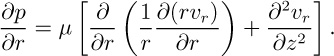
If vz is the local axial velocity, prove that the corresponding increase of pressure from just inside the free surface (pR) to the centerline (p0) is:

where β = vzL/vz0. Obtain an expression for the ratio ξ =(pR − p0)/(μdvz/dz), in which the denominator is the pressure decrease due to viscosity when crossing the interface from the air into the filament, and which was accounted for in Example 6.6.
Estimate ξ at the beginning of the filament for the situation in which μ =104 P, L = 1 m, RL (exit radius) = 0.0002 m, vz0 = 0.02 m/s, and vzL = 2 m/s. Comment briefly on your findings.
28. Condenser with varying viscosity—M. In a condenser, a viscous liquid flows steadily under gravity as a uniform laminar film down a vertical cooled flat plate. Due to conduction, the liquid temperature T varies linearly across the film, from T0 at the cooled plate to T1 at the hotter liquid/vapor interface, according to T = T0 + y(T1 − T0)/h. The viscosity of the liquid is given approximately by μ = μ*(1 − αT ), where μ* and α are constants.
Prove that the viscosity at any location can be reexpressed as:
where μ0 and μ1 are the viscosities at temperatures T0 and T1, respectively.
What is the expression for the shear stress τyx for a liquid for steady flow in the x direction? Derive an expression for the velocity vx as a function of y. Make sure that you do not base your answer on any equations that assume constant viscosity.
Sketch the velocity profile for both a small and a large value of α.
29. Rotating sphere—M. A sphere of radius R, immersed in a liquid of viscosity μ of infinite extent, rotates about its z axis (see Fig. 5.9(b)) with a steady angular velocity ω in the ϕ direction. You may assume that the only nonzero liquid velocity component is that in the ϕ direction, and is of the form vϕ = c sin θ/r2.
(a) Verify that the proposed form for vϕ satisfies the appropriate momentum balance, and determine c in terms of R and ω.
(b) Prove that the shear stress at any radial location in the liquid is τrϕ = −3μc sin θ/r3, and carefully explain the minus sign.
(c) Obtain an expression for the torque T needed to rotate the sphere, as a function of R, ω, and μ. You should need the indefinite integral:

30. Moving plate—M. Similar to the first part of Example 6.4, consider a viscous fluid of infinite extent and kinematic viscosity ν with a long flat plate in its surface. At t = 0, the plate suddenly starts moving with a steady velocity vx0 in the x direction. Prove, by checking ∂vx/∂t = ν∂2vx/∂z2 and the boundary conditions, that the fluid velocity at a depth z is subsequently given by:
You may assume that:

31. Oscillating plate—M. Similar to the second part of Example 6.4, consider a viscous fluid of infinite extent and kinematic viscosity ν with a long flat plate in its surface. The plate oscillates backwards and forwards in the x direction with velocity vx0 = a sin ωt. After any initial transients have died out, prove, by checking ∂vx/∂t = ν∂2vx/∂z2 and the boundary conditions, that the fluid velocity at a depth z is subsequently given by:
in which
32. True/false. check true or false, as appropriate:
(a) For horizontal flow of a liquid in a rectangular duct between parallel plates, the pressure varies linearly both in the direction of flow and in the direction normal to the plates.
T ![]() F
F ![]()
(b) For horizontal flow of a liquid in a rectangular duct between parallel plates, the boundary conditions can be taken as zero velocity at one of the plates and either zero velocity at the other plate or zero velocity gradient at the centerline.
T ![]() F
F ![]()
(c) For horizontal flow of a liquid in a rectangular duct between parallel plates, the shear stress varies from zero at the plates to a maximum at the centerline.
T ![]() F
F ![]()
(d) For horizontal flow of a liquid in a rectangular duct between parallel plates, a measurement of the pressure gradient enables the shear-stress distribution to be found.
T ![]() F
F ![]()
(e) In fluid mechanics, when integrating a partial differential equation, you get one or more constants of integration, whose values can be determined from the boundary condition(s).
T ![]() F
F ![]()
(f) For flows occurring between r = 0 and r = a in cylindrical coordinates, the term ln r may appear in the final expression for one of the velocity components.
T ![]() F
F ![]()
(g) For flows in ducts and pipes, the volumetric flow rate can be obtained by differentiating the velocity profile.
T ![]() F
F ![]()
(h) Natural convection is a situation whose analysis depends on not taking the density as constant everywhere.
T ![]() F
F ![]()
(i) A key feature of the Weissenberg rheogoniometer is the fact that a conical upper surface results in a uniform velocity gradient between the cone and the plate, for all values of radial distance.
T ![]() F
F ![]()
(j) If, in three dimensions, the pressure obeys the equation ∂p/∂y = −ρg, and both ∂p/∂x and ∂p/∂z are nonzero, then integration of this equation gives the pressure as p = −ρgy + c, where c is a constant.
T ![]() F
F ![]()
(k) If two immiscible liquids A and B are flowing in the x direction between two parallel plates, both the velocity vx and the shear stress τyx are continuous at the interface between A and B, where the coordinate y is normal to the plates.
T ![]() F
F ![]()
(l) In compression molding of a disk between two plates, the force required to squeeze the plates together decreases as time increases.
T ![]() F
F ![]()
(m) For flow in a wetted-wall column, the pressure increases from atmospheric pressure at the gas/liquid interface to a maximum at the wall.
T ![]() F
F ![]()
(n) For one-dimensional flow in a pipe—either laminar or turbulent—the shear stress τrz varies linearly from zero at the wall to a maximum at the centerline.
T ![]() F
F ![]()
(o) In Example 6.1, for flow between two parallel plates, the shear stress τyx is negative in the upper half (where y > 0), meaning that physically it acts in the opposite direction to that indicated by the convention.
T ![]() F
F ![]()