
Chapter 2. Mass, Energy, And Momentum Balances
2.1 General Conservation Laws
THE study of fluid mechanics is based, to a large extent, on the conservation laws of three extensive quantities:
1. Mass—usually total, but sometimes of one or more individual chemical species.
2. Total energy—the sum of internal, kinetic, potential, and pressure energy.
3. Momentum, both linear and angular.
For a system viewed as a whole, conservation means that there is no net gain nor loss of any of these three quantities, even though there may be some redistribution of them within a system. A general conservation law can be phrased relative to the general system shown in Fig. 2.1, in which can be identified:
Fig. 2.1. (a) System and its surroundings; (b) transfers to and from a system. For a chemical reaction, creation and destruction terms would also be included inside the system.

1. The system V.
2. The surroundings S.
3. The boundary B, also known as the control surface, across which the system interacts in some manner with its surroundings.
The interaction between system and surroundings is typically by one or more of the following mechanisms:
1. A flowing stream, either entering or leaving the system.
2. A “contact” force on the boundary, usually normal or tangential to it, and commonly called a stress.
3. A “body” force, due to an external field that acts throughout the system, of which gravity is the prime example.
4. Useful work, such as electrical energy entering a motor or shaft work leaving a turbine.
Let X denote mass, energy, or momentum. Over a finite time period, the general conservation law for X is:
Nonreacting system
For a mass balance on species i in a reacting system
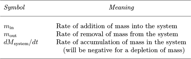
The symbols are defined in Table 2.1. The understanding is that the creation and destruction terms, together with the superscript i, are needed only for mass balances on species i in chemical reactions, which will not be pursued further in this text.
Table 2.1. Meanings of Symbols in Equation (2.1)

It is very important to note that Eqn. (2.1a) cannot be applied indiscriminately, and is only observed in general for the three properties of mass, energy, and momentum. For example, it is not generally true if X is another extensive property such as volume, and is quite meaningless if X is an intensive property such as pressure or temperature.
In the majority of examples in this book, it is true that if X denotes mass and the density is constant, then Eqn. (2.1a) simplifies to the conservation of volume, but this is not the fundamental law. For example, if a gas cylinder is filled up by having nitrogen gas pumped into it, we would very much hope that the volume of the system (consisting of the cylinder and the gas it contains) does not increase by the volume of the (compressible) nitrogen pumped into it!
Equation (2.1a) can also be considered on a basis of unit time, in which case all quantities become rates; for example, ΔXsystem becomes the rate, dXsystem/dt, at which the X-content of the system is increasing, xin (note the lower-case “x”) would be the rate of transfer of X into the system, and so on, as in Eqn. (2.2):
2.2 Mass Balances
The general conservation law is typically most useful when rates are considered. In that case, if X denotes mass M and x denotes a mass “rate” m (the symbol ![]() can also be used) the transient mass balance (for a nonreacting system) is:
can also be used) the transient mass balance (for a nonreacting system) is:
in which the symbols have the meanings given in Table 2.2.
Table 2.2. Meanings of Symbols in Equation (2.3)
The majority of the problems in this text will deal with steady-state situations, in which the system has the same appearance at all instants of time, as in the following examples:
1. A river, with a flow rate that is constant with time.
2. A tank that is draining through its base, but is also supplied with an identical flow rate of liquid through an inlet pipe, so that the liquid level in the tank remains constant with time.
Steady-state problems are generally easier to solve, because a time derivative, such as dMsystem/dt, is zero, leading to an algebraic equation.
A few problems—such as that in Example 2.1—will deal with unsteady-state or transient situations, in which the appearance of the system changes with time, as in the following examples:
1. A river, whose level is being raised by a suddenly elevated dam gate downstream.
2. A tank that is draining through its base, but is not being supplied by an inlet stream, so that the liquid level in the tank falls with time.
Transient problems are generally harder to solve, because a time derivative, such as dMsystem/dt, is retained, leading to a differential equation.
The tank shown in Fig. E2.1(a) has a volume V =1m3 and contains air that is maintained at a constant temperature by being in thermal equilibrium with its surroundings.
Fig. E2.1. (a) Tank evacuation.
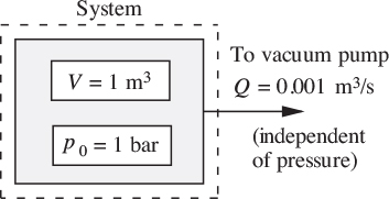
If the initial absolute pressure is p0 = 1 bar, how long will it take for the pressure to fall to a final pressure of 0.0001 bar if the air is evacuated at a constant rate of Q = 0.001 m3/s, at the pressure prevailing inside the tank at any time?
Solution
First, and fairly obviously, choose the tank as the system, shown by the dashed rectangle. Note that there is no inlet to the system, and just one outlet from it. A mass balance on the air in the system (noting that a rate of loss is negative) gives:

Note that since the tank volume V is constant, dV/dt = 0. For an ideal gas:
so that:
Cancellation of M/RT gives the following ordinary differential equation, which governs the variation of pressure p with time t:
Separation of variables and integration between t = 0 (when the pressure is p0) and a later time t (when the pressure is p) gives:

Fig. E2.1. (b) Exponential decay of tank pressure.
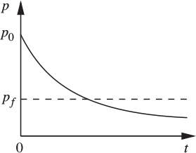
The resulting solution shows an exponential decay of the tank pressure with time, also illustrated in Fig. E2.1(b):
Thus, the time tf taken to evacuate the tank from its initial pressure of 1 bar to a final pressure of pf =0.0001 bar is:

Problem 2.1 contains a variation of the above, in which air is leaking slowly into the tank from the surrounding atmosphere.
Steady-state mass balance for fluid flow
A particularly useful and simple mass balance—also known as the continuity equation—can be derived for the situation shown in Fig. 2.2, where the system resembles a wind sock at an airport. At station 1, fluid flows steadily with density ρ1 and a uniform velocity u1 normally across that part of the surface of the system represented by the area A1. In steady flow, each fluid particle traces a path called a streamline. By considering a large number of particles crossing the closed curve C, we have an equally large number of streamlines that then form a surface known as a stream tube, across which there is clearly no flow. The fluid then leaves the system with uniform velocity u2 and density ρ2 at station 2, where the area normal to the direction of flow is A2.
Fig. 2.2. Flow through a stream tube.

Referring to Eqn. (2.3), there is no accumulation of mass because the system is at steady state. Therefore, the only nonzero terms are m1 (the rate of addition of mass) and m2 (the rate of removal of mass), which are equal to ρ1A1u1 and ρ2A2u2, respectively, so that Eqn. (2.3) becomes:

which can be rewritten as:
where m (= m1 = m2) is the mass flow rate entering and leaving the system.
For the special but common case of an incompressible fluid, ρ1 = ρ2, so that the steady-state mass balance becomes:
in which Q is the volumetric flow rate.
Equations (2.4a/b) would also apply for nonuniform inlet and exit velocities, if the appropriate mean velocities um1 and um2 were substituted for u1 and u2. However, we shall postpone the concept of nonuniform velocity distributions to a more appropriate time, particularly to those chapters that deal with microscopic fluid mechanics.
2.3 Energy Balances
Equation (2.1) is next applied to the general system shown in Fig. 2.3, it being understood that property X is now energy. Observe that there is both flow into and from the system. Also note the quantities defined in Table 2.3.
Fig. 2.3. Energy balance on a system with flow in and out.

Table 2.3. Definitions of Symbols for Energy Balance

A differential energy balance results by applying Eqn. (2.1) over a short time period. Observe that there are two transfers into the system (incoming mass and heat) and two transfers out of the system (outgoing mass and work). Since the mass transfers also carry energy with them, there results:
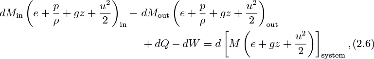
in which each term has units of energy or work. In the above, the system is assumed for simplicity to be homogeneous, so that all parts of it have the same internal, potential, and kinetic energy per unit mass; if such were not the case, integration would be needed throughout the system. Also, multiple inlets and exits could be accommodated by means of additional terms.
Since the density ρ is the reciprocal of v, the volume per unit mass, e + p/ρ = e + pv, which is recognized as the enthalpy per unit mass. The flow energy term p/ρ in Eqn. (2.6), also known as injection work or flow work, is readily explained by examining Fig. 2.4. Consider unit mass of fluid entering the stream tube under a pressure p1. The volume of the unit mass is:
which is the product of the area A1 and the distance 1/ρ1A1 through which the mass moves. (Here, the “1” has units of mass.) Hence, the work done on the system by p1 in pushing the unit mass into the stream tube is the force p1A1 exerted by the pressure multiplied by the distance through which it travels:
Likewise, the work done by the system on the surroundings at the exit is:
Fig. 2.4. Flow of unit mass to and from stream tube.

Steady-state energy balance
In the following, all quantities are per unit mass flowing. Referring to the general system shown in Fig. 2.5, the energy entering with the inlet stream plus the heat supplied to the system must equal the energy leaving with the exit stream plus the work done by the system on its surroundings. Therefore, the right-hand side of Eqn. (2.6) is zero under steady-state conditions, and division by dMin = dMout gives:

in which each term represents an energy per unit mass flowing.
Fig. 2.5. Steady-state energy balance.

For an infinitesimally small system in which differential changes are occurring, Eqn. (2.10) may be rewritten as:

in which, for example, de is now a differential change, and v =1/ρ is the volume per unit mass.
Now examine the increase in internal energy de, which arises from frictional work dF dissipated into heat, heat addition dq from the surroundings, less work pdv done by the fluid. That is: de = dF + dq − pdv. Thus, eliminate the change de in the internal energy from Eqn. (2.11), and expand the term d(pv),

which simplifies to the differential form of the mechanical energy balance, in which heat terms are absent:

For a finite system, for flow from point 1 to point 2, Eqn. (2.13) integrates to:

in which a finite change is consistently the final minus the initial value, for example:
An energy balance for an incompressible fluid of constant density permits the integral to be evaluated easily, giving:

In the majority of cases, g will be virtually constant, in which case there is a further simplification to:

which is a generalized Bernoulli equation, augmented by two extra terms—the frictional dissipation, F, and the work w done by the system. Note that F can never be negative—it is impossible to convert heat entirely into useful work. The work term w will be positive if the fluid flows through a turbine and performs work on the environment; conversely, it will be negative if the fluid flows through a pump and has work done on it.
Power
The rate of expending energy in order to perform work is known as power, with dimensions of ML2/T3, typical units being W (J/s) and ft lbf/s. The relations in Table 2.4 are available, depending on the particular context.
Table 2.4. Expressions for Power in Different Systems
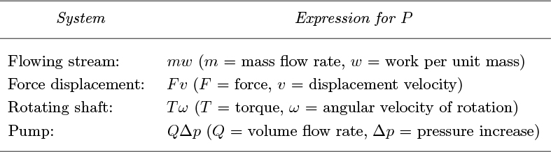
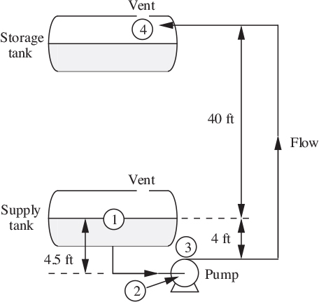
Fig. E2.2 shows an arrangement for pumping n-pentane (ρ = 39.3 lbm/ft3)at 25 °C from one tank to another, through a vertical distance of 40 ft. All piping is 3-in. I.D. Assume that the overall frictional losses in the pipes are given (by methods to be described in Chapter 3) by:

For simplicity, however, you may ignore friction in the short length of pipe leading to the pump inlet. Also, the pump and its motor have a combined efficiency of 75%. If the mean velocity um is 25 ft/s, determine the following:
(a) The power required to drive the pump.
(b) The pressure at the inlet of the pump, and compare it with 10.3 psia, which is the vapor pressure of n-pentane at 25 °C.
(c) The pressure at the pump exit.
Solution
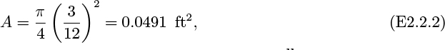
The cross-sectional area of the pipe and the mass flow rate are:
Since the supply tank is fairly large, the liquid/vapor interface in it is descending only very slowly, so that u1 . = 0. An energy balance between points 1 and 4 (where both pressures are atmospheric, so that Δp = 0) gives:


Hence, the work per unit mass flowing is:

in which the minus sign indicates that work is done on the liquid. The power required to drive the pump motor is:
The pressure at the inlet to the pump is obtained by applying Bernoulli’s equation between points 1 and 2:

Since the pipe has the same diameter throughout (3 in.), the velocity u2 entering the pump is the same as that in the vertical section of pipe, 25 ft/s. Solving for the pressure at the pump inlet,
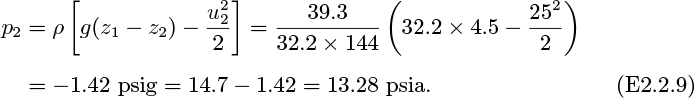
(For better accuracy, friction in the short length of pipe between the tank and the pump inlet should be included, particularly in the context of Chapter 3; however, it will be fairly small and we are justified in ignoring it here.) Note that p2 is above the vapor pressure of n-pentane, which therefore remains as a liquid as it enters the pump. If p2 were less than 10.3 psia, the n-pentane would tend to vaporize and the pump would not work because of cavitation.
The pressure at the pump exit is most readily found by applying an energy balance across the pump. Since there is no change in velocity (the inlet and outlet lines have the same diameter), and no frictional pipeline dissipation:
But p2 = −1.42 psig, w = −3,163 ft2/s2, and Δz =0.5 ft, so that:
The same result could have been obtained by applying the energy balance between points 3 and 4.
2.4 Bernoulli’s Equation
Situations frequently occur in which the following simplifying assumptions can reasonably be made:
1. The flow is steady.
2. There are no work effects; that is, the fluid neither performs work (as in a turbine) nor has work performed on it (as in a pump). Thus, w = 0 in Eqn. (2.17).
3. The flow is frictionless, so that F = 0 in Eqn. (2.17). Clearly, this assumption would not hold for long runs of pipe.
4. The fluid is incompressible; that is, the density is constant. This approximation is excellent for the majority of liquids, and may also be reasonable for some cases of gas flows provided that the pressure variations are moderately small.
Under these circumstances, the general energy balance reduces to: Δ

which is the famous Bernoulli’s equation, one of the most important relations in fluid mechanics.
For flow between points 1 and 2 on the same streamline, or for any two points in a fluid under static equilibrium (in which case the velocities are zero), Eqn. (2.18) becomes:

which states that although the kinetic, potential, and pressure energies may vary individually, their sum remains constant. Each term in (2.19) must have the same dimensions as the first one, namely, velocity squared or L2/T2. Further manipulations in the two principal systems of units yield the following:
1. SI Units
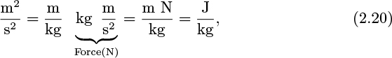
which is readily seen to be energy per unit mass.
2. English Units

which is again energy per unit mass. However, since the poundal is an archaic unit of force, each term in Bernoulli’s equation may be divided by the conversion factor gc ft lbm/lbf s2 if the more practical lbf is required in numerical calculations. For example, the kinetic energy term then becomes:

As previously indicated, we prefer not to include gc—or any other conversion factors—directly in these equations.
Head of fluid
A quantity closely related to energy per unit mass may be obtained by dividing (2.19) through by the gravitational acceleration g:
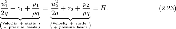
Each term in (2.23) has dimensions of length, and indeed the terms such as u21/2g, z1, p1/ρg, and H are called the velocity head, static head, pressure head, and total head, respectively.
A physical interpretation of fluid head is readily available by considering the steady flow of a liquid from a tank through the idealized frictionless pipe shown in Fig. 2.6(a). At point 1 (the free surface), the velocity u1 is virtually zero for a tank of reasonable size, and the pressure p1 there is also zero (gauge) because the free surface is exposed to the atmosphere. Thus, the velocity and pressure heads are both zero at point 1, so that the total head (H for example) is identical with the static head z1, namely, the elevation of the free surface relative to some datum level. Hence, Eqn. (2.23) can be rewritten as:
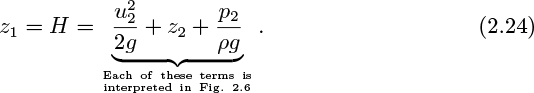
Looking now at point 2, the static head is simply the elevation z2 of that point above the datum level; the pressure head is the height above point 2 to which the liquid rises in the manometer—an amount that is just sufficient to balance the pressure p2; and, by difference, the elevation difference between the top of the liquid in the tube and point 1 must be the velocity head u22/2g.
Fig. 2.6. (a) Physical interpretation of velocity, static, and pressure heads for pipe flow, and (b) pressure head increase across a pump.
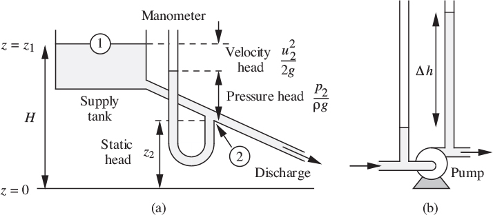
Since the pipe diameter is constant, continuity also requires the velocity and hence the velocity head u22/2g to be constant. Referring to Fig. 2.6(a), since the static head continuously decreases along the pipe, and the total head is constant, the pressure head must constantly increase. But since the pressure at the exit— or very shortly after it—is atmospheric, the pressure head must again be zero! The reader will doubtless ask: “Is there an anomaly?”, and may wish to ponder whether or not the diagram is completely accurate as drawn.
Fig. 2.6(b) shows that the pressure increase Δp across a pump is also equivalent to a head increase Δh =Δp/ρg, being the increase in liquid levels in piezometric tubes placed at the pump inlet and exit.
Note carefully that the above analysis is for an ideal liquid—one that exhibits no friction. In practice, there would be some loss in total head along the pipe.
2.5 Applications of Bernoulli’s Equation
We now apply Eqn. (2.18) to several commonly occurring situations, in which useful relations involving pressures, velocities, and elevations may be obtained. The usual assumptions of steady flow, no external work, no friction, and constant density may reasonably be made in each case.
Tank draining
First, consider Fig. 2.7, in which a tank is draining through an orifice of cross-sectional area A in its base. If the orifice is rounded, the streamlines will be parallel with one another at the exit and the pressure will be uniformly atmospheric there. The elevation of the free surface at point 1 is h above the orifice, where z2 is taken to be zero. There are no work effects between 1 and 2, and the fluid is incompressible. Also, because the liquid is descending quite slowly, there is essentially no frictional dissipation (unless the liquid is very viscous) and the flow is virtually steady. Hence, Eqn. (2.19) can be applied between 1 and 2, giving:

Fig. 2.7. Tank draining through a rounded orifice.

But u1 = 0 if the cross-sectional area of the tank is appreciably larger than that of the orifice; also, p1 = p2, since both are atmospheric pressure. Equation (2.25) then reduces to:
so the exit velocity of the liquid is exactly commensurate with a free fall under gravity through a vertical distance h. The corresponding volumetric flow rate is:
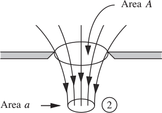
However, if the orifice is sharp-edged with area A, as shown in Fig. 2.8, the cross-sectional area of the jet continues to contract after it leaves the orifice because of its inertia to a value a at a location, known as the vena contracta,1 where the streamlines are parallel to one another. In this case, if Cc is the coefficient of contraction, the following relations give the area of the vena contracta and the total flow rate:
1 Latin for “constricted jet.”
in which the coefficient of contraction is found in most instances to have the value:
Fig. 2.8. Contraction of the jet through a sharp-edged orifice.
Orifice-plate “meter.”
The Bernoulli principle—of a decrease in pressure in an accelerated stream—can be employed for the measurement of fluid flow rates in the device shown in Fig. 2.9. There, an orifice plate consisting of a circular disc with a central hole of area Ao is bolted between the flanges on two sections of pipe of cross-sectional area A1.
Fig. 2.9. Flow through an orifice plate.

Bernoulli’s equation applies to the fluid as it flows from left to right through the orifice of a reduced area because it is found experimentally that a contracting stream is relatively stable, so that frictional dissipation can be ignored, especially over such a short distance. Hence, as the velocity increases, the pressure decreases. The following theory demonstrates that by measuring the pressure drop p1 − p2, it is possible to determine the upstream velocity u1. Let u2 be the velocity of the jet at the vena contracta.
Bernoulli’s equation applied between points 1 and 2, which have the same elevation (z1 = z2), gives:

Conservation of mass between points 1 and 2 gives the continuity equation:
Elimination of u2 between Eqns. (2.31) and (2.32) gives:

Solution for u1 yields:

so that the volumetric flow rate Q is:
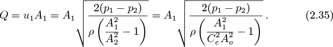
In Eqn. (2.35), the coefficient of contraction Cc is approximately 0.63 in most cases. However, the following version, which is somewhat less logical than Eqn. (2.35) and uses a dimensionless discharge coefficient CD, is used in practice instead:

Fig. 2.10 shows how CD varies with two additional dimensionless groups, namely, the ratio of the orifice diameter to the pipe diameter, and the Reynolds number through the orifice:
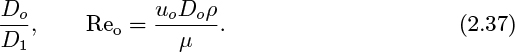
It is easy to show that the Reynolds number at the orifice is given in terms of the upstream Reynolds number Re1 (which is usually more readily available) by the relation:

Downstream of the vena contracta, the jet is found experimentally to become unstable as it expands back again to the full cross-sectional area of the pipe; the subsequent turbulence and loss of useful work means that Bernoulli’s equation cannot be used in the downstream section.
Fig. 2.10. Discharge coefficient for orifice plates. Based on values from G.G. Brown et al., Unit Operations, John Wiley & Sons, New York, 1950.
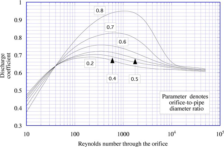
This type of result—the expression of one dimensionless group in terms of one or more additional dimensionless groups—will occur many times throughout the text, and will be treated more generally in Section 4.5 on dimensional analysis. For the moment, however, the reader should note that these dimensionless groups typically represent the ratio of one quantity to a similarly related quantity. The orifice-to-pipe diameter ratio has an obvious geometrical interpretation, stating how large the orifice is in relation to the pipe. The significance of the Reynolds number is not so obvious, but represents the ratio of an inertial effect (given by ρu2, for example), to a viscous effect (already given in Eqn. (1.14) by the product of viscosity and a velocity gradient—μu/D, for example); thus, the ratio of these two quantities is (ρu2)/(μu/D)= ρuD/μ, the Reynolds number. Chapters 3 and 4 emphasize that turbulence is more likely to occur at higher Reynolds numbers.
Pitot tube
The device shown in Fig. 2.11 is also based on the Bernoulli principle, and is used for finding the velocity of a moving craft such as a boat or an airplane. Here, the Pitot tube is attached to a boat, for example, which is moving steadily with an unknown velocity u1 through otherwise stagnant water of density ρ. The submerged tip of the tube faces the direction of motion; the pressure at the tip can be found from the height h to which the water rises in the tube or—more practically—by a pressure transducer (see Section 2.7).
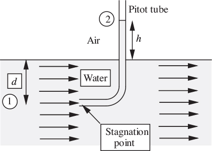
For simplicity, consider the motion relative to an observer on the boat, in which case the Pitot tube is effectively stationary, with water approaching it with an upstream velocity u1. Opposite the Pitot tube, the oncoming water decelerates and comes to rest at the stagnation point at the tip of the tube.
Application of Bernoulli’s equation between points 1 and 2 gives:

in which the first zero recognizes the datum level z1 = 0 at point 1, and the second zero indicates that the water is stagnant with u2 = 0 at point 2. But from hydrostatics, the pressure at point 1 is:
Subtraction of Eqn. (2.40) from Eqn. (2.39) gives:
so that the velocity u1 of the boat is readily determined from the height of the water in the tube. In practice, a pressure transducer would probably be used for monitoring the excess pressure (corresponding to ρgh) instead of measuring the water level, but we have retained the latter because it is conceptually simpler.
A very similar device, called the Pitot-static tube, is shown in Fig. 2.12, and is employed for measuring the velocity at different radial locations in a pipe. Here, two tubes are involved. The left-hand tube simply measures the pressure and the movable right-hand one is essentially a Pitot tube as before. The velocity u1 at the particular transverse location where the Pitot tube is placed is given by:
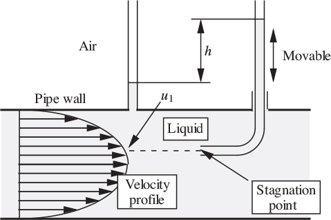
Fig. E2.3. Tank filling from river: (a) before pipe is submerged; (b) after pipe is submerged.
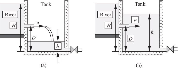
Fig. E2.3 shows a concrete tank that is to be filled with water from an adjacent river in order to provide a supply of water for the sprinklers on a golf course. The level of the river is H = 10 ft above the base of the tank, and the short connecting pipe, which offers negligible resistance, discharges water at a height D = 4 ft above the base of the tank. The inside cross-sectional area of the pipe is a = 0.1 ft2, and that of the tank is A = 1,000 ft2. Derive an algebraic expression for the time t taken to fill the tank, and then evaluate it for the stated conditions.
Solution
The solution is in two parts—before and after the pipe is submerged under the water in the tank, corresponding to (a) and (b) in Fig. E2.3. In both cases, the (gauge) atmospheric pressure is zero.
Part 1. Here, the flow rate is constant, since the water level in the tank is below the pipe outlet and hence offers no resistance to the flow. Bernoulli’s equation, applied between the surface of the water in the river and the pipe discharge to the atmosphere, gives:
so that:
The volumetric flow rate is constant at ua, and the time for the water to reach the level of the pipe is the gain in volume divided by the flow rate:

Part 2. For the submerged pipe, as in Fig. E2.3(b), the flow rate is now variable, because it is influenced by the level in the tank. The discharge pressure equals the hydrostatic pressure ρg(h − D) due to the water in the tank above the discharge point. Bernoulli’s equation, again applied between the surface of the water in the river and the pipe discharge, yields:

or
A volumetric balance (the density is constant) equates the flow rate into the tank to the rate of increase of volume of water in the tank:
Separation of variables and integration (see Appendix A for a wide variety of standard forms) gives:
The filling time for Part 2 is therefore:
The total filling time is obtained by adding Eqns. (E2.3.3) and (E2.3.7):
2.6 Momentum Balances
Momentum
The general conservation law also applies to momentum M, which for a mass M moving with a velocity u, as in Fig. 2.13(a), is defined by:
Strangely, there is no universally accepted symbol for momentum. In this text and elsewhere, the symbols M and m (or ![]() ) frequently denote mass and mass flow rate, respectively. Therefore, we arbitrarily denote momentum and the rate of transfer of momentum due to flow by the symbols M (“script” M) and
) frequently denote mass and mass flow rate, respectively. Therefore, we arbitrarily denote momentum and the rate of transfer of momentum due to flow by the symbols M (“script” M) and ![]() , respectively. Momentum is a vector quantity, and for the simple case shown has the direction of the velocity u. More generally, there may be velocity components ux, uy, and uz (sometimes also written as vx, vy, and vz, or as u, v, and w) in each of the three coordinate directions, illustrated for Cartesian coordinates in Fig. 2.13(b). In this case, the momentum of the mass M has components Mux, Muy, and Muz in the x, y, and z directions.
, respectively. Momentum is a vector quantity, and for the simple case shown has the direction of the velocity u. More generally, there may be velocity components ux, uy, and uz (sometimes also written as vx, vy, and vz, or as u, v, and w) in each of the three coordinate directions, illustrated for Cartesian coordinates in Fig. 2.13(b). In this case, the momentum of the mass M has components Mux, Muy, and Muz in the x, y, and z directions.
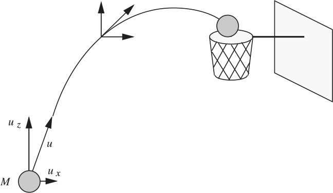
Fig. 2.13. (a) Momentum as a product of mass and velocity; (b) velocity components in the three coordinate directions.

For problems in more than one dimension, conservation of momentum or a momentum balance applies in each of the coordinate directions. For example, for the basketball shown in Fig. 2.14, momentum Mux in the x direction remains almost constant (drag due to the air would reduce it slightly), whereas the upward momentum Muz is constantly diminished—and eventually reversed in sign—by the downward gravitational force.
Fig. 2.14. Momentum varies with time in the x and y directions.
If a system, such as a river, consists of several parts each moving with different velocities u (boldface denotes a vector quantity), the total momentum of the system is obtained by integrating over all of its mass:
Law of momentum conservation
Following the usual law, Eqn. (2.2), the net rate of transfer of momentum into a system equals the rate of increase of the momentum of the system. The question immediately arises: “How can momentum be transferred?” The answer is that there are two principal modes, by a force and by convection, as follows in more detail.
1. Momentum Transfer by a Force
A force is readily seen to be equivalent to a rate of transfer of momentum by examining its dimensions:
In fluid mechanics, the most frequently occurring forces are those due to pressure (which acts normal to a surface), shear stress (which acts tangentially to a surface), and gravity (which acts vertically downwards). Pressure and stress are examples of contact forces, since they occur over some region of contact with the surroundings of the system. Gravity is also known as a body force, since it acts throughout a system.
A momentum balance can be applied to a mass M falling with instantaneous velocity u under gravity in air that offers negligible resistance. Considering momentum as positive downwards, the rate of transfer of momentum to the system (the mass M) is the gravitational force Mg, and is equated to the rate of increase of downwards momentum of the mass, giving:

Note that M can be taken outside the derivative only if the mass is constant. The acceleration is therefore:
and, although this is a familiar result, it nevertheless follows directly from the principle of conservation of momentum.
Another example is provided by the steady flow of a fluid in a pipe of length L and diameter D, shown in Fig. 2.15. The upstream pressure p1 exceeds the downstream pressure p2 and thereby provides a driving force for flow from left to right. However, the shear stress τw exerted by the wall on the fluid tends to retard the motion.
Fig. 2.15. Forces acting on fluid flowing in a pipe.

A steady-state momentum balance to the right (note that a direction must be specified) is next performed. As the system, choose for simplicity a cylinder that is moving with the fluid, since it avoids the necessity of considering flows entering and leaving the system. The result is:

Here, the first term is the rate of addition of momentum to the system resulting from the net pressure difference p1−p2, which acts on the circular area πD2/4. The second term is the rate of subtraction of momentum from the system by the wall shear stress, which acts to the left on the cylindrical area πDL. Since the flow is steady, there is no change of momentum of the system with time, and dM/dt =0. Simplification gives:
which is an important equation from which the wall shear stress can be obtained from the pressure drop (which is easy to determine experimentally) independently of any constitutive equation relating the stress to a velocity gradient.
2. Momentum Transfer by Convection or Flow
The convective transfer of momentum by flow is more subtle, but can be appreciated with reference to Fig. 2.16, in which water from a hose of cross-sectional area A impinges with velocity u on the far side of a trolley of mass M with (for simplicity) frictionless wheels. The dotted box delineates a stationary system within which the momentum Mv is increasing to the right, because the trolley clearly tends to accelerate in that direction. The reason is that momentum is being transferred across the surface BC into the system by the convective action of the jet. The rate of transfer is the mass flow rate m = ρuA times the velocity u, namely:
which is again momentum per unit time.
Fig. 2.16. Convection of momentum.
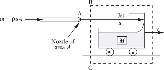
The acceleration of the trolley will now be found by applying momentum balances in two different ways, depending on whether the control volume is stationary or moving. In each case, the water leaves the nozzle of cross-sectional area A with velocity u and the trolley has a velocity v. Both velocities are relative to the nozzle. The reader should make a determined effort to understand both approaches, since momentum balances are conceptually more difficult than mass and energy balances. It is also essential to perform the momentum balance in an inertial frame of reference—one that is either stationary or moving with a uniform velocity, but not accelerating.
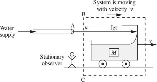
1. Control surface moving with trolley. As shown in Fig. 2.17, the control surface delineating the system is moving to the right at the same velocity v as the trolley. The observer perceives water entering the system across BC not with velocity u but with a relative velocity (u − v), so that the rate m of convection of mass into the control volume is:
Fig. 2.17. Stationary observer—moving system.
A momentum balance (positive direction to the right) gives:
Note that to obtain the momentum flux, m is multiplied by the absolute velocity u [not the relative velocity (u − v), which has already been accounted for in the mass flux m]. Also, the mass of the system is not constant, but is increasing at a rate given by:
It follows from the last three equations that the acceleration a = dv/dt of the trolley to the right is:
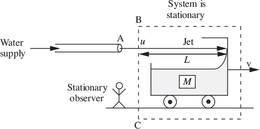
2. Control volume fixed. In Fig. 2.18, the control surface is now fixed in space, so that the trolley is moving within it. Also—and not quite so obviously, that part of the jet of length L inside the control surface is lengthening at a rate dL/dt = v and increasing its momentum ρALu, and this must of course be taken into account. A mass balance first gives:
Rate of addition of mass = Rate of increase of mass,
Likewise, a momentum balance gives:
Rate of addition = Rate of increase.
Fig. 2.18. Stationary observer—fixed system.
By eliminating dM/dt between Eqns. (2.56) and (2.57) and rearranging, the acceleration becomes identical with that in (2.55), thus verifying the equivalence of the two approaches:
Fig. E2.4 shows a plan of a jet of water impinging against a shield that is held stationary by a force F opposing the jet, which divides into several radially outward streams, each leaving at right angles to the jet. If the total water flow rate is Q = 1 ft3/s and its velocity is u = 100 ft/s, find F (lbf).
Fig. E2.4. Jet impinging against shield.

Solution
Perform a momentum balance to the right on the system bounded by the dotted control surface. If the mass flow rate is m, the rate of transfer of momentum into the system by convection is mu. The exiting streams have no momentum to the right. Also, the opposing force amounts to a rate of addition of momentum F to the left. Hence, at steady state:
so that:
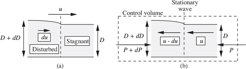
As shown in Fig. E2.5(a), a small disturbance in the form of a wave of slightly increased depth D + dD travels with velocity u along the surface of a layer of otherwise stagnant water of depth D. Note that no part of the water itself moves with velocity u—just the dividing line between the stagnant and disturbed regions; in fact, the water velocity just upstream of the front is a small quantity du, and downstream it is zero. If the viscosity is negligible, find the wave velocity in terms of the depth.
Fig. E2.5. (a) Moving wave front; (b) stationary wave front as seen by observer traveling with wave.
Estimate the warning times available to evacuate communities that are threatened by the following “avalanches” of water:
(a) A tidal wave (closely related to a tsunami2), generated by an earthquake 1,000 miles away, traveling across an ocean of average depth 2,000 ft.
2 According to The New York Times of December 27, 2004, a tsunami is a series of waves generated by underwater seismic disturbances. In the disaster of the previous day, the Indian tectonic plate slipped under (and raised) the Burma plate off the coast of Sumatra. The article reported that the ocean floor could rise dozens of feet over a distance of hundreds of miles, displacing unbelievably enormous quantities of water. The waves reached Indonesia, Thailand, Sri Lanka, and elsewhere, causing immense destruction and the eventual loss of more than 225,000 lives.
(b) An onrush, caused by a failed dam 50 miles away, traveling down a river of depth 12 ft that is also flowing towards the community at 4 mph.
Solution
As shown in Fig. E2.5(a), the problem is a transient one, since the picture changes with time as the wave front moves to the right. The solution is facilitated by superimposing a velocity u to the left, as in Fig. E2.5(b)—that is, by taking the viewpoint of an observer traveling with the wave, who now “sees” water coming from the right with velocity u and leaving to the left with velocity u − du.
All forces, flow rates, and momentum fluxes will be based on unit width normal to the plane of the figure. Because the disturbance is small, second-order differentials such as (dD)2 and du dD can be neglected. Referring to Fig. E2.5(b), the total downstream and upstream pressure forces are obtained by integration:

A mass balance on the indicated control volume relates the downstream and upstream velocities and their depths (remember that calculations are based on unit width, so D × 1= D is really an area):
Since the viscosity is negligible, there is no shear stress exerted by the floor on the water above. Therefore, a steady-state momentum balance to the left on the control volume yields: 1 2
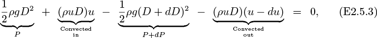
which simplifies to:
Substitution for dD from the mass balance yields the velocity u of the wave:
Note that the wave velocity increases in proportion to the square root of the depth of the water. Another viewpoint is that the Froude number, Fr = u2/gD, being the ratio of inertial (ρu2) to hydrostatic (ρgD) effects, is unity.
The calculations for the water “avalanches” now follow:
(a) Ocean wave:
so that the warning time is:

(a) River wave:

Since the river is itself flowing at 4 mph, the total wave velocity is 13.4+4 = 17.4 mph. Thus, the warning time is:
The velocity of a sinusoidally varying wave traveling on deep water is discussed in Section 7.10.
Further momentum balances for an orifice plate and sudden expansion
This section concludes with two examples in which pressure changes in turbulent zones, where Bernoulli’s equation cannot be applied, are determined from momentum balances.
Fig. 2.19 shows the flow through an orifice plate. Mass balances yield the following (note that A1 = A3):
Fig. 2.19. Overall pressure drop across an orifice plate.

or:

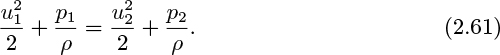
In the upstream section, where the streamlines are converging and the flow is relatively frictionless, Bernoulli’s equation has already been used to relate changes in pressure to changes in velocity:
Elimination of u2 between (2.60) and (2.61) gives the pressure drop in the upstream section:

In the downstream section, it is characteristic of a jet of expanding cross-sectional area that it generates excessive turbulence, so that the frictional dissipation term F is no longer negligible and Bernoulli’s equation cannot be applied. However, the length of pipe between 2 and 3 is sufficiently small so that the wall shear stress imposed by it can be ignored. A momentum balance (positive to the right) on the dotted control volume between locations 2 and 3 gives:
Here, the first two terms correspond to convection of momentum into and from the control volume; the second two terms reflect the pressure forces on the two ends, both of area A1. Although there will be some fluctuations of momentum within the system because of the turbulence, these variations will essentially cancel out over a sufficiently long time period; this quasi steady-state viewpoint says that the flow is steady in the mean. The eddies surrounding the jet at the vena contracta keep recirculating and the net momentum transfer from them across the control surface is zero.
The pressure drop in the downstream section is obtained by eliminating u3 between Eqns. (2.60) and (2.63):

The overall pressure drop is found by adding Eqns. (2.62) and (2.64):

Observe that the last term in Eqn. (2.65), being the product of two squares, must always be positive. Hence, p3 is always less than p1, and there is overall a
loss of useful work. Indeed, the corresponding frictional dissipation term F can be found by employing the overall energy balance, Eqn. (2.17), between points 1 and 3:

Here, the first, second, and fourth terms are zero because overall there is no change in velocity, no elevation change, and zero work performed. The frictional dissipation per unit mass flowing is therefore:

which value can then be used for an inclined or even vertical pipe, the effect of elevation being accounted for by the gΔz term.
The following questions also deserve reflection:
1. Is p3 less than, equal to, or greater than p2? Why?
2. What is involved in performing a momentum balance between points 1 and 2?
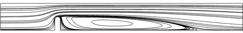
A CFD (computational fluid dynamics) simulation of highly turbulent flow through an orifice plate is presented in Example 9.4 in Chapter 9. To show the power of CFD, the lower half of a small part of that simulation is shown in Fig. 2.20. Note the remarkable similarity to the earlier qualitative sketch of Fig. 2.19.
Fig. 2.20. Streamlines computed by COMSOL Multiphysics for flow from left to right through an orifice plate—see Example 9.4.
A sudden expansion in a pipeline shown in Fig. 2.21 occurs when two pipes of different diameters are joined together. The corresponding F term is obtained by a momentum balance similar to that in the downstream section of the orifice plate, and is left as an exercise (see Problem P2.22).
Fig. 2.21. Sudden expansion in a pipe.
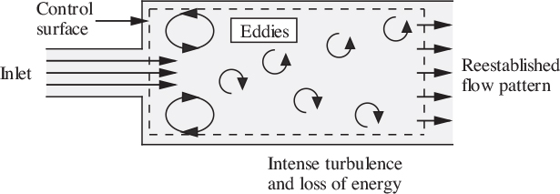
Fig. E2.6(a) shows a flow-measuring instrument called a rotameter, consisting typically of a solid “float” (made of an inert material such as stainless steel, glass, or tantalum) inside a gradually tapered glass tube. As the fluid flows upward, the float reaches a position of equilibrium, from which the flow rate can be read from the adjacent scale, which is often etched on the glass tube.
Fig. E2.6. (a) Section of rotameter, and (b) control volume.
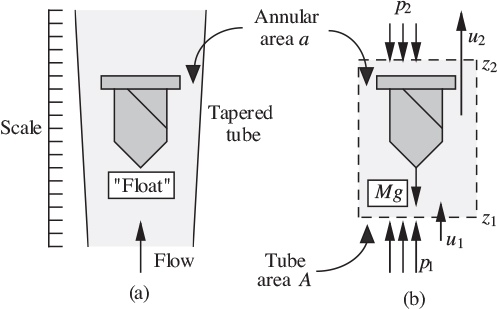
The float is often stabilized by helical grooves incised into it, which induce rotation—hence the name. Other shapes of floats—including spheres in the smaller instruments—may be employed. The problem is to analyze the flow and the equilibrium position of the float. Assume that viscous effects are unimportant, which is true for the majority of industrially important fluids as they pass around the float.
Solution
Some flow-measuring devices, such as the orifice plate and Venturi meter, incorporate a fixed reduction of area, which produces a pressure drop that depends on the flow rate. In contrast, the rotameter depends on the change of an annular area a between the float and the tube, which is a function of the vertical location of the float, to yield an essentially fixed pressure drop at all flow rates. In other words, the annular area functions as an orifice of variable area.
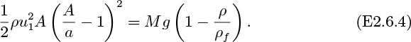
Referring to Fig. E2.6(b), mass, energy, and upward momentum balances yield:

in which ρ and ρf are the densities of the fluid and the float, respectively. In the momentum balance, the three types of terms are indicated by underbraces, and the bracketed expression is the volume of fluid in the control volume. Starting with Eqn. (E2.6.3), terms involving the pressures and elevations can be eliminated by using Eqn. (E2.6.2) and terms involving m and u2 can be eliminated by using Eqn. (E2.6.1), leading after some algebra to:
The flow rate is then:
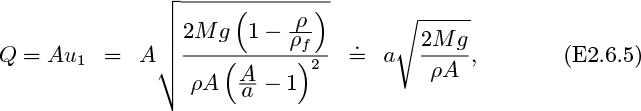
in which the approximate form holds for aℓ A and ρℓ ρf . Since a = a(z) and A = A(z) depend on the location z of the float, Eqn. (E2.6.5) demonstrates that the flow rate can be determined from the equilibrium position of the float. In practice, since a is not known precisely (there may be a vena contracta effect), Eqn. (E2.6.5) can be used for a preliminary design, the rotameter being subsequently calibrated before accurate use.
Angular momentum
So far, we have been concerned with the conservation of momentum in a specified linear direction. However, it is also possible to consider angular momentum, which is introduced by examining Fig. 2.22(a), in which a differential mass dM is rotating with angular velocity ω rad/s in an arc having a radius of curvature r. The angular momentum dA of the mass is defined as:
Fig. 2.22. (a) Mass moving in arc of radius r; (b) integration to find the total angular momentum.
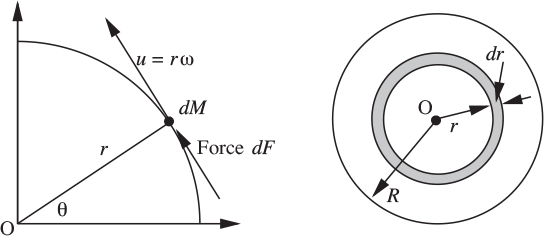
For a finite distributed mass, the total angular momentum is obtained by integration over the entire mass:

in which the moment of inertia I is defined as:
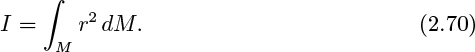
For example, for the flywheel of width W , radius R, and mass M, whose cross section is shown in Fig. 2.21(b):
Also, torque, being the product of a force times a radius, is given in differential and integrated form by:

and is analogous to force in linear momentum problems and will result in a transfer of angular momentum. In the same way that the application of a force F to a constant mass M moving with velocity v leads to the law F = Mdv/dt, one form of an angular momentum balance is:
Here, T is the torque applied to the axle of the flywheel whose moment of inertia is I, resulting in an angular acceleration dω/dt.
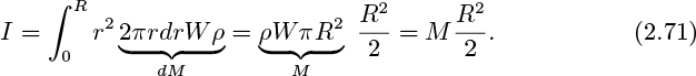
As a final example, consider the impeller of a centrifugal pump, whose cross section is shown in Fig. 2.23. (For practical reasons, the vanes are usually curved, not straight, as discussed further in Section 4.2.)
Fig. 2.23. Cross section of pump impeller.
The impeller rotates with angular velocity ω, and its rotation causes the fluid to be thrown radially outwards between the vanes by centrifugal action (again, see Section 4.2). The fluid enters at a radial position r1 and leaves at a radial position r2; the corresponding tangential velocities u1 and u2 denote the inlet and exit liquid velocities relative to a stationary observer. The arrows A, B, C, and D illustrate the liquid velocity relative to the rotating impeller.
An angular momentum balance on the impeller gives:
For steady operation, the derivative is zero, and the torque required to rotate the impeller is:
Here, m is the mass flow rate through the pump, subscripts 1 and 2 denote inlet and exit conditions, and u = rω denotes the corresponding tangential velocities. The corresponding power needed to drive the pump is the product of the angular velocity and the torque (see also Table 2.4):
2.7 Pressure, Velocity, and Flow Rate Measurement
Previous sections have alluded to various ways of measuring the most important quantities associated with static and flowing fluids. This section reviews and amplifies such methods. Excellent and comprehensive surveys are available in a book and on a CD.3
3 See R.J. Goldstein, ed., Fluid Mechanics Measurements, 2nd ed., Hemisphere Publishing Corporation,
Pressure
A piezometer is the generic name given to a pressure-measuring device. Three basic types are recognized here; in each case, learning from the principle of the Pitot tube, it is important that the opening to the device be tangential to any fluid motion, otherwise an erroneous reading will result.
New York, 1996; and Material Balances & Visual Equipment Encyclopedia of chemical Engineering Equipment, CD produced by the Multimedia Education Laboratory, Department of chemical Engineering, University of Michigan, Susan Montgomery (Director), 2002.
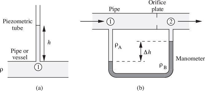
1. Transparent tubes can be connected to the point(s) where the pressure is needed, two examples being given in Fig. 2.24:
(a) In the piezometric tube, the height to which the liquid rises is observed, and the required gauge pressure at point 1 in the pipe or vessel is p1 = ρgh. Fairly obviously, this arrangement can only be used if the fluid is a liquid and not a gas.
(b) For measuring a pressure difference, such as occurs across an orifice plate, a differential “U” manometer can be employed, using a liquid that is immiscible with the one whose pressure is desired (and which may now be either a liquid or a gas). The arrangement shown is for ρB >ρA, and the required pressure difference is p1 − p2 =(ρB − ρA)gΔh. For ρB <ρA, the manometer tube would be an inverted “U” and would be placed above the pipe. The manometer can also be employed in situation (a) if the right-hand leg is vented to the atmosphere, in which case the fluid whose pressure is needed can then be a gas.
Fig. 2.24. (a) piezometric tube, and (b) manometer.
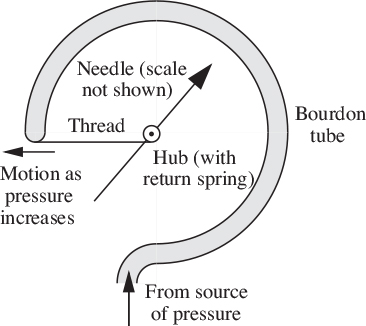
2. The Bourdon gauge, of which the essentials are illustrated in Fig. 2.25 (the linkage to the needle is actually more intricate), employs a curved, flattened metal tube, open at one end and closed at the other. Pressure applied to the open end tends to cause the tube to straighten out, and this motion is transmitted to a needle that rotates and points to the appropriate reading on a circular scale.
Fig. 2.25. Elements of Bourdon tube pressure gauge.
3. The pressure transducer employs a small thin diaphragm, usually contained in a hollow metallic cylinder that is “plugged” into the location where the pressure is needed. Variations of pressure cause the diaphragm to bend, and the extent of such distortion can be determined by different methods. For example, piezoresistive and piezoelectric material properties of either the diaphragm or another sensing element bonded to it will cause variations in the strain to be translated into variations in the electrical resistance or electric polarization, either of which can be converted into an electrical signal for subsequent processing. Advances in semiconductor fabrication have allowed a wide variety of pressure transducers to become readily available, and these are clearly the preferred instruments if the pressure is to be recorded or transmitted to a process-control computer.
Velocity
Fluid velocities can be determined by several methods, some of the more important being:
1. Tracking of small particles or bubbles moving with the fluid. By photographing over a known short time period, the velocity can be deduced from the distance traveled by a particle. For flow inside a transparent pipe, the distance of the particle from the wall can be determined either by focusing closely on a known location or, better, by using stereoscopic photography with two cameras and comparing the apparent particle locations on the resulting two negatives. Laser-Doppler velocimetry (LDV) determines the velocity by measuring the Doppler shift of a laser beam caused by the moving microscopic particle. Infrared lasers are used for assessing upper-atmosphere turbulence.
2. Pitot tube measurements, as already discussed.
3. Hot-wire anemometry, in which a very small and thin electrically heated wire suspended between two supports is introduced into the moving stream. Measurements are made of the resistance of the wire, which depends on its temperature, which is governed by the local heat-transfer coefficient, which in turn depends on the local velocity.
Flow rate
The following is a representative selection of the wide variety of methods and instruments for measuring flow rates of fluids.
1. Discharge of the flowing stream into a receptacle so that the volume or mass of fluid flowing during a known period of time can be measured directly.
2. Devices based on the Bernoulli principle, in which the pressure decreases because of an increased velocity through a restriction. Examples are the orifice plate and rotameter already discussed, and the Venturi (see Problem 2.12).
3. Flow of a liquid over a weir or notch, in which the depth of the liquid depends on the flow rate.
4. Turbine meter, consisting of a small in-line turbine placed inside a section of pipe; the rotational speed, which can be transmitted electrically to a recorder, depends on the flow rate.
5. Thermal flow meter, in which a small heater is located between two temperature detectors—one (A) upstream and the other (B) downstream of the heater. For a given power input, the temperature difference (TB −TA) is measured and will vary inversely with the flow rate, which can then be determined.
6. Target meter, typically consisting of a disk mounted on a flexible arm and placed normal to the flow in a pipe. The displacement of the disk, and hence the flow rate, is determined from the output of a strain gauge attached to the arm.
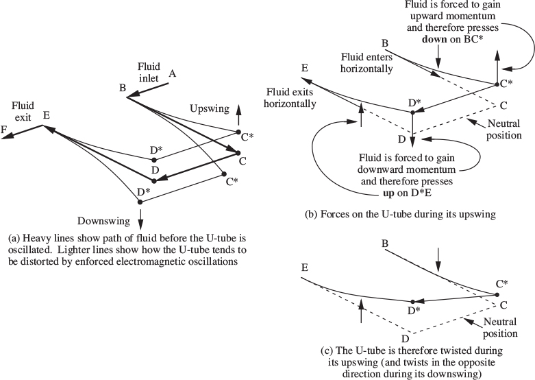
7. Coriolis flow meter. Here—see Fig. 2.26(a)—the fluid is forced to flow through a slightly flexible U-tube BCDE (with suitably rounded corners) that is vibrated up and down by a magnetic driver. Fig. 2.26(b) examines what happens when the U-tube is in the “upswing” position. Suppose that the orientation is such that the fluid enters horizontally. Because the fluid is forced to conform to the path BC* it acquires some vertically upward momentum and therefore exerts an opposite or downward force on the leg BC*. And because it must lose this vertical momentum before it leaves the U-tube at E, the fluid exerts an upward force on the leg D*E. The net result (Fig. 2.26(c)) is that—seen from the CD end—the U-tube twists clockwise while in the upswing mode. And when it is in the downswing mode, exactly the opposite rotation occurs. Electromagnetic sensors near the two long arms of the U-tube detect the magnitude of the twisting motion, which depends on the mass flow rate of the fluid. The instrument is therefore useful for measuring mass flow rates even though the fluid may be non-Newtonian and possibly contain some gas bubbles. It is called a Coriolis meter because it can also be analyzed by considering the forces on a moving fluid in a rotating or oscillating system of coordinates.
Fig. 2.26. Principles of a Coriolis mass-flow meter.
8. Vortex-shedding meter. An obstacle is placed in the flowing stream, and vortices are shed on alternate sides of the wake. The frequency of shedding, and hence the flow rate, is determined by various methods, one of which measures the oscillations of a flexible strip placed in the wake.
Problems for Chapter 2
1. Evacuation of leaking tank—M . This problem concerns the tank shown in Fig. P2.1 and is the same as Example 2.1, except that there is now a small leak into the tank from the outside air, whose pressure is 1 bar. The mass flow rate of the leak equals c(ρ0 − ρ), where c = 10−5 m3/s is a constant, ρ0 is the density of the ambient air, and ρ is the density of the air inside the tank. The initial density of air inside the tank is also ρ0.
What is the lowest attainable pressure p* inside the tank? How long will it take the pressure to fall halfway from its initial value to p*?
Fig. P2.1. Evacuation of tank with a leak.

2. Slowed traffic—E . A two-lane highway carries cars traveling at an average speed of 60 mph. In a construction zone, where the cars have merged into one lane, the average speed is 20 mph and the average distance between front bumpers of successive cars is 25 ft. What is the average distance between front bumpers in each lane of the two-lane section? Why? How many cars per hour are passing through the construction zone?
3. “Density” of cars—E . While driving down the expressway at 65 mph, you count an average of 18 cars going in the other direction for each mile you travel. At any instant, how many cars are there per mile traveling in the opposite direction to you?
4. Ethylene pipeline—E . Twenty lbm/s of ethylene gas (assumed to behave ideally) flow steadily at 60 °F in a pipeline whose internal diameter is 8 in. The pressure at upstream location 1 is p1 = 60 psia, and has fallen to p2 = 25 psia at downstream location 2. Why does the pressure fall, and what are the velocities of the ethylene at the two locations?
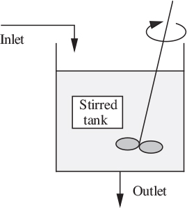
5. Transient behavior of a stirred tank—E . The well-stirred tank of volume V = 2 m3 shown in Fig. P2.5 is initially filled with brine, in which the initial concentration of sodium chloride at t = 0 is c0 = 1 kg/m3. Subsequently, a flow rate of Q = 0.01 m3/s of pure water is fed steadily to the tank, and the same flow rate of brine leaves the tank through a drain. Derive an expression for the subsequent concentration of sodium chloride c in terms of c0, t, Q, and V . Make a sketch of c versus t and label the main features. How long (minutes and seconds) will it take for the concentration of sodium chloride to fall to a final value of cf =0.0001 kg/m3?
Fig. P2.5. Stirred tank with continuous flow.
6. Stirred tank with crystal dissolution—M . A well-stirred tank of volume V =2m3 is filled with brine, in which the initial concentration of sodium chloride at t =0 is c0 = 1 kg/m3. Subsequently, a flow rate of Q = 0.01 m3/s of pure water is fed steadily to the tank, and the same flow rate of brine leaves the tank through a drain. Additionally, there is an ample supply of sodium chloride crystals in the bottom of the tank, which dissolve at a uniform rate of m = 0.02 kg/s.
Why is it reasonable to suppose that the volume of brine in the tank remains constant? Derive an expression for the subsequent concentration c of sodium chloride in terms of c0, m, t, Q, and V . Make a sketch of c versus t and label the main features. Assuming an inexhaustible supply of crystals, what will the concentration c of sodium chloride in the tank be at t = 0, 10, 100, and ∞ s? Carefully define the system on which you perform a transient mass balance.
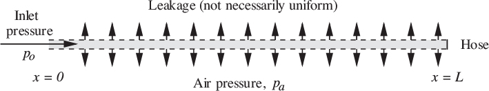
7. Soaker garden hose—D. A “soaker” garden hose with porous canvas walls is shown in Fig. P2.7. Water is supplied at a pressure p0 at x = 0, and the far end at x = L is blocked off with a cap. At any intermediate location x, water leaks out through the wall at a volumetric rate q = β(p − pa) per unit length, where p is the local pressure inside the hose and the constant β and the external air pressure pa are both known.
Fig. P2.7. A garden hose with porous walls.
You may assume that the volumetric flow rate of water inside the hose is proportional to the negative of the pressure gradient:
where the constant α is also known. (Strictly speaking, Eqn. (P2.7.1) holds only for laminar flow, which may or may not be the case—see Chapter 3 for further details.) By means of a mass balance on a differential length dx of the hose, prove that the variations of pressure obey the differential equation:
where P =(p − pa) and γ2 = β/α. Show that:
satisfies Eqn. (P2.7.2), and determine the constants A and B from the boundary conditions. Hence, prove that the variations of pressure are given by: p − pa p0 − pa
Then show that the total rate of loss of water from the hose is given by:
Finally, sketch (p − pa)/(p0 − pa) versus x for low, intermediate, and high values of γ. Point out the main features of your sketch.
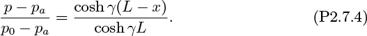
8. Performance of a siphon—E . As shown in Fig. P2.8, a pipe of cross-sectional area A =0.01 m2 and total length 5.5 m is used for siphoning water from a tank. The discharge from the siphon is 1.0 m below the level of the water in the tank. At its highest point, the pipe rises 1.5 m above the level in the tank. What is the water velocity v (m/s) in the pipe? What is the lowest pressure in bar (gauge), and where does it occur? Neglect pipe friction. Are your answers reasonable?
Fig. P2.8. Siphon for draining tank.
If the siphon reaches virtually all the way to the bottom of the tank (but is not blocked off), is the time taken to drain the tank equal to t = V/vA, where V is the initial volume of water in the tank, and v is still the velocity as computed above when the tank is full? Explain your answer.
9. Pitot tube—E . The speed of a boat is measured by a Pitot tube. When traveling in seawater (ρ =64lbm/ft3), the tube measures a pressure of 2.5 lbf/in2 due to the motion. What is the speed (mph) of the boat? What would be the speed in fresh water (ρ = 62.4 lbm/ft3), also for a pressure of 2.5 lbf/in2?
10. Leaking carbon dioxide—M . A long vertical tube is open at the top and contains a small orifice in its base, which is otherwise closed. The lower 10-m section of the tube is filled with carbon dioxide (MW = 44). Otherwise, there is air (MW = 28.8) above the carbon dioxide in the tube and also outside the tube. Calculate the velocity (m/s) of carbon dioxide that issues from the orifice. In which direction does it flow?
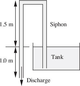
11. Two pressure gauges—E . Fig. P2.11 shows two pressure gauges that are mounted on a vertical water pipe 40 ft apart, yet they read exactly the same pressure, 100 psig.
(a) Is the water flowing? Why?
(b) If so, in which direction is it flowing? Why? Hint: You may wish to use an overall energy balance in the pipe between the two gauges to check your answer.
Fig. P2.11. Two pressure gauges.
12. Venturi “meter”—M . A volumetric flow rate Q of liquid of density ρ flows through a pipe of cross-sectional area A, and then passes through the Venturi “meter” shown in Fig. P2.12, whose “throat” cross-sectional area is a. A manometer containing mercury (ρm) is connected between an upstream point (station 1) and the throat (station 2), and registers a difference in mercury levels of Δh. Derive an expression giving Q in terms of A, a, g, Δh, ρ, ρm, and CD.

If the diameters of the pipe and the throat of the Venturi are 6 in. and 3 in. respectively, what flow rate (gpm) of iso-pentane (ρ = 38.75 lbm/ft3) would register a Δh of 20 in. on a mercury (s = 13.57) manometer? What is the corresponding pressure drop in psi? Assume a discharge coefficient of CD = 0.98. Note: Those parts of the manometer not occupied by the mercury are filled with iso-pentane, since there is free communication with the pipe via the pressure tappings.
13. Orifice plate—M . A horizontal 2-in. I.D. pipe carries kerosene at 100 °F, with density 50.5 lbm/ft3 and viscosity 3.18 lbm/ft hr. In order to measure the flow rate, the line is to be fitted with a sharp-edged orifice plate, with pressure tappings that are connected to a mercury manometer that reads up to a 15-in. difference in the mercury levels. If the largest flow rate of kerosene is expected to be 560 lbm/min, specify the diameter of the orifice plate that would then just register the full 15-in. difference between the mercury levels.
14. Tank draining—M . A cylindrical tank of diameter 1 m has a well-rounded orifice of diameter 2 cm in its base. How long will it take an initial depth of acetone equal to 2 m to drain completely from the tank? How long would it take if the orifice were sharp-edged? If needed, the density of acetone is 49.4 lbm/ft3.
Fig. P2.15. Draining tank with oil and water.
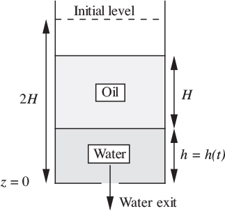
15. Draining immiscible liquids from a tank—M . Fig. P2.15 shows a tank of cross-sectional area A that initially (t = 0) contains two layers, each of depth H: oil (density ρo), and water (ρw). A sharp-edged orifice of cross-sectional area a and coefficient of contraction 0.62 in the base of the tank is then opened. Derive an expression for the time t taken for the water to drain from the tank, in terms of H, g, A, a, ρo, and ρw. Neglect friction and assume that Aℓ a. You should need one of the integrals given in Appendix A.
Fig. P2.16. Cylindrical liquid-storage tank.

16. Draining a horizontal cylindrical tank—D. A cylindrical tank of radius r and length L, vented at the top to the atmosphere, is shown in side and end elevations in Fig. P2.16. Initially (t = 0), it is full of a low-viscosity liquid, which is then allowed to drain through an exit pipe of length H and cross-sectional area A.
Prove that the time taken to drain just the tank (excluding the exit pipe) is:
If L =5 m, r =1 m, H = 1 m, what value of A will enable the tank to drain in one hour? If necessary, use Simpson’s rule to approximate the integral.
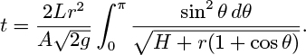
17. Lifting silicon wafers—M . Your supervisor has suggested the device shown in Fig. P2.17 for picking up delicate circular silicon wafers without touching them. A mass flow rate m of air of constant density ρ at a pressure p0 is blown down a central tube of radius r1, which is connected to a flange of external radius r2. The device is positioned at a distance H above the silicon wafer, also of radius r2, that is supposedly to be picked up. The air flows radially outwards with radial velocity ur(r) in the gap and is eventually discharged to the atmosphere at a pressure p2, which is somewhat lower than p0.
Fig. P2.17. Picking up a silicon wafer.
If the flow is frictionless and gravitational effects may be neglected:
(a) Obtain an expression for ur in terms of the radial position r and any or all of the given parameters. Sketch a graph that shows how ur varies with r between radial locations r1 and r2.
(b) What equation relates the velocity and pressure in the air stream to each other? Sketch another graph that shows how the pressure p(r) in the gap between the flange and wafer varies with radial position between r1 and r2. Hint: it may be best to work backwards, starting with a pressure p2 at radius r2. Clearly indicate the value p0 on your graph.
(c) Comment on the likely merits of the device for picking up the wafer.
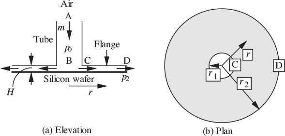
18. Rocket performance—M . Fig. P2.18 shows a rocket whose mass is M lbm and whose vertical velocity at any instant is v ft/s. A propellant is being ejected downwards through the exhaust nozzle with a mass flow rate m lbm/s and a velocity u ft/s relative to the rocket. The gravitational acceleration is g ft/s2 and the rocket experiences a drag force F = kv2 lbmft/s2, where k is a known constant.
Fig. P2.18. Rocket traveling upward.
(a) What is the absolute downward velocity of the propellant leaving the exhaust nozzle?
(b) What is the flux of momentum downward through the nozzle?
(c) Is the mass of the rocket constant?
(d) Perform a momentum balance on the moving rocket as the system. Make it quite clear whether your viewpoint is that of an observer on the ground or one traveling with the rocket. Hence, derive a formula for the rocket acceleration dv/dt, in terms of M, m, v, u, and k.
19. Jet airplane—E . A small jet airplane of mass 10,000 kg is in steady level flight at a velocity of u = 250 m/s through otherwise stationary air (ρa = 1.0 kg/m3). The outside air enters the engines, where it is burned with a negligible amount of fuel to produce a gas of density ρg = 0.40 kg/m3, which is discharged at atmospheric pressure with velocity v = 600 m/s relative to the airplane through exhaust ports with a total cross-sectional area of 1 m2. Calculate:
(a) The mass flow rate (kg/s) of gas.
(b) The frictional drag force (N) due to air resistance on the external surfaces of the airplane.
(c) The power (W) of the engine.
20. Jet-propelled boat—M . As shown in Fig. P2.20, a boat of mass M =1,000 lbm is propelled on a lake by a pump that takes in water and ejects it, at a constant velocity of v = 30 ft/s relative to the boat, through a pipe of cross-sectional area A = 0.2 ft2. The resisting force F of the water is proportional to the square of the boat velocity u, which has a maximum value of 20 ft/s.
What is the acceleration of the boat when its velocity is u = 10 ft/s? For a stationary observer on the lakeshore, use two approaches for a momentum balance and check that they give the same result. (Take a control volume large enough so that the water ahead of the boat is undisturbed.)
(a) A control surface moving with the boat.
(b) A control surface fixed in space, within which the boat is moving. The power for propelling the boat is known to be:
where m is the mass flow rate of water through the pump. Explain this result as simply as possible from the viewpoint of an observer traveling with the boat. Give a reason why the power P decreases as the velocity u of the boat increases!
Fig. P2.20. Jet-propelled boat.

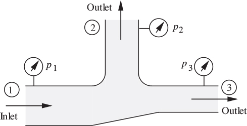
21. Branch pipe—M . The system shown in Fig. P2.21 carries crude oil of specific gravity 0.8. The total volumetric flow rate at point 1 is 10 ft3/s. Branches 1, 2, and 3 are 5, 4, and 3 inches in diameter, respectively. All three branches are in a horizontal plane, and friction is negligible. The pressure gauges at points 1 and 3 read p1 = 25 psig and p3 = 20 psig, respectively. What is the pressure at point 2? (Hint: Note that Bernoulli’s equation can only be applied to one streamline at a time!)
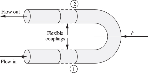
22. Sudden expansion in a pipe—M . Fig. P2.22 shows a sudden expansion in a pipe. Why can’t Bernoulli’s equation be applied between points 1 and 2, even though the flow pattern is fully established at both locations?
Prove that there is an overall increase of pressure equal to:
Where does the energy come from to provide this pressure increase? Also prove that the frictional dissipation term is:

Fig. P2.22. Sudden expansion in a pipe.

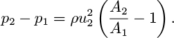
23. Force on a return elbow—M . Fig. P2.23 shows an idealized view of a return elbow or “U-bend,” which is connected to two pipes by flexible hoses that transmit no forces. Water flows at a velocity 10 m/s through the pipe, which has an internal diameter of 0.1 m. The gauge pressures at points 1 and 2 are 3.0 and 2.5 bar, respectively. What horizontal force F (N, to the left) is needed to keep the return elbow in position?
Fig. P2.23. Flow around a return elbow.
24. Hydraulic jump—M . Fig. P2.24 shows a hydraulic jump, which sometimes occurs in open channel or river flow. Under the proper conditions, a rapidly flowing stream of liquid suddenly changes to a slowly flowing or tranquil stream with an attendant rise in the elevation of the liquid surface.
By using mass and momentum balances on control volumes that extend unit distance normal to the plane of the figure, neglecting friction at the bottom of the channel, and assuming the velocity profiles to be flat, prove that the downstream depth d2 is given by:

If u1 = 5 m/s and d1 = 0.2 m, what are the corresponding downstream values? (An overall energy balance—not required here—will show that the viscous or frictional loss F per unit mass flowing is positive only for the direction of the jump as shown; hence, a deep stream cannot spontaneously change to a shallow stream.)

25. Reducing elbow—M . Fig. P2.25 shows a reducing elbow located in a horizontal plane (gravitational effects are unimportant), through which a liquid of constant density is flowing. The flexible connections, which do not exert any forces on the elbow, serve only to delineate the system that is to be considered; they would not be used in practice, because the retaining forces Fx and Fy would be provided by the walls of the pipe.
Neglecting frictional losses, derive expressions for the following, in terms of any or all of the known inlet gauge pressure p1, inlet velocity u1, inlet and exit diameters D1 and D2 (and hence the corresponding cross-sectional areas A1 and A2), and liquid density ρ:
(a) The exit velocity u2 and pressure p2.
(b) The retaining forces Fx and Fy needed to hold the elbow in position. Calculate the two forces Fx and Fy if D1 = 0.20 m, D2 = 0.15 m, p1 = 1.5 bar (gauge), u1 = 5.0 m/s, and ρ =1,000 kg/m3 (the liquid is water).
26. Jet-ejector pump—M . Water from a supply having a total head of 100 ft is used in the jet of an ejector, shown in Fig. P2.26, in order to lift 10 ft3/s of water from another source (at a lower level) that has a total head of −5 ft.

The nozzle area of the jet pipe is 0.05 ft2 and the annular area of the suction line at section 1 is 0.5 ft2. Determine the volumetric flow rate from the 100-ft head supply and the total delivery head for the ejector at section 2.
27. Speed of a sound wave—M . As shown in Fig. P2.27(a), a sound wave is a very small disturbance that propagates through a medium; its wave front, which moves with velocity c, separates the disturbed and undisturbed portions of the medium. (No part of the fluid itself actually moves with a velocity c.) In the undisturbed medium, the velocity is u = 0, the pressure is p, and the density is ρ. Just behind the wave front, in the disturbed medium, these values have been changed by infinitesimally small amounts, so that the corresponding values are du, p + dp, and ρ + dρ. The system is best analyzed from the viewpoint of an observer traveling with the wave front, as shown in Fig. P2.27(b), which is obtained by superimposing a velocity c to the left, so the wave front is now stationary, and the flow is steady, from right to left.
Fig. P2.27. Propagation of sound wave; (a) relative to a stationary observer; (b) relative to an observer traveling with the wave front.

By appropriate steady-state mass and momentum balances on a control volume, which you should clearly indicate, prove that the velocity of sound is:

(Although not needed here, it may further be shown that the above derivative should be evaluated at constant entropy.)
28. Car retarding force—M . Experimentally, how would you most easily determine the total retarding force (wind, road, etc.) on a car at various speeds?
Fig. P2.29. Plan of garden sprinkler.

29. Garden sprinkler, arms rotating—E . Fig. P2.29 shows an idealized plan of a garden sprinkler. The central bearing is well lubricated, so the arms are quite free to rotate about the central pivot. Each of the two nozzles has a cross-sectional area of 5 sq mm, and each arm is 20 cm long. Why is there rotation in the indicated direction? If the water supply rate to the sprinkler is 0.0001 m3/s, determine:
(a) The velocity u (m/s) of the water jets relative to the nozzles.
(b) The angular velocity of rotation, ω, of the arms, in both rad/s and rps.
30. Garden sprinkler, arms fixed—E . Consider again the sprinkler of Problem 2.29. For the same water flow rate, what applied torque is needed to prevent the arms from rotating?
31. Oil/water separation—M . Design a piece of equipment, as simple as possible, that will separate, by settling, a stream of an oil/water mixture into two individual streams of oil and water, as sketched in Fig. P2.31 (where the relative levels are not necessarily correct).
Fig. P2.31. Unit for separating oil and water.
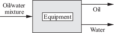
Adhere to the following specifications:
(a) The exit streams are at atmospheric pressure.
(b) Anticipate that the inlet stream will fluctuate with time in both its oil and water content, with upper flow rate limits of 10 and 40 gpm, respectively.
(c) To insure proper separation, the residence time in the equipment of both the oil and water should be, on average, at least 20 minutes. For each phase, the residence time is defined as t = V/Q, the volume V occupied by the phase divided by its volumetric flow rate Q.
(d) A small relative water flow rate should not cause oil to leave through the water outlet, nor should a small relative oil flow rate cause water to leave through the oil outlet.
Your answer should specify the following details, at least:
(a) The volume and shape of the equipment.
(b) The locations of the inlet and exit pipes.
(c) The internal configuration.
32. Slowing down of the earth—D. If a and b are the semi-major and semi-minor axes, respectively, consider the ellipse whose equation is:
Consider the ellipsoid, shown in Fig. P2.32, formed by rotating the ellipse about its minor axis. Write down expressions for the mass dM and moment of inertia dI (about the semi-minor axis) for the disk of radius x and thickness dy shown in the figure. Hence, prove that the mass and moment of inertia of the ellipsoid are:
Fig. P2.32. Rotating ellipsoid.

At midnight on December 31, 1995, an extra second was added to all cesium-133 atomic clocks to align them more closely with time as measured by the earth’s rotational speed, which had been declining. Twenty such “leap” seconds were added in the twenty-four years from 1972 to 1995. One theory for the slowing down is that the earth is gradually bulging at the equator and flattening at the poles.4 Assuming that the earth was a perfect sphere in 1972, and was in 1995 an ellipsoid, by what fraction of its original radius had it changed at the equator and at the poles? If the earth’s radius is 6.37 × 10⁶ m, what are the corresponding distances?
4 Curt Suplee, “Setting Earth’s clock,” Washington Post, December 31, 1990. See also Dava Sobel, “The 61-second minute,” New York Times, December 31, 1995.
33. Head for a real liquid—M . Fig. 2.6 gave an interpretation of fluid heads for an ideal, frictionless liquid. For a real liquid, in which pipe friction is significant, redraw the diagram and explain all of its features. Incorporate four equally spaced manometer locations, starting at the entrance to the pipe and finishing at its exit.
34. Acceleration of a jet airplane—M . Fig. P2.34 shows an airplane of mass M that is flying horizontally with velocity u through otherwise stationary air. The airplane is propelled by a jet engine that ejects hot gas of density ρg at atmospheric pressure with velocity v relative to the engine, through exhaust ports of total cross-sectional area A. The drag force F is cu2, where c is a known constant.
Fig. P2.34. Airplane in horizontal flight.
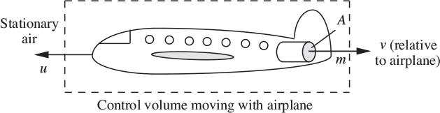
Answer the following, using any or all of the symbols u, v, ρg, A, M, and c, as already defined:
(a) Write down an expression for m, the mass flow rate of hot gas leaving the engines.
(b) As “seen” by a stationary observer on the ground, what is the velocity and direction of the exhaust gases?
(c) Perform a momentum balance on a control surface moving with the airplane, and derive an expression for its acceleration a. Assume that the mass of fuel consumed is negligibly small in comparison with that of the air passing through the engine.
(d) Compute a (m/s2) if u = 100 m/s, v = 300 m/s, ρg =0.4 kg/m3, A =2 m2, M =104 kg, and c =0.60 kg/m.
35. Performance of a “V-notch”—M . Fig. P2.35(a) shows a “V-notch,” which is a triangular opening of half-angle θ cut in the end wall of a tank or channel carrying a liquid. We wish to deduce the volumetric flow rate Q of liquid spilling over the notch from the height H of the free surface above the bottom of the notch.
Fig. P2.35. Discharge over a V-notch.

The side elevation, Fig. P2.35(b), shows a representative streamline, flowing horizontally at a constant depth h below the free surface, between an upstream point 1 (where the pressure is hydrostatic and the velocity negligibly small) to a downstream point 2 at the notch exit, where the pressure is atmospheric (all the way across the section A–A). What is the reason for supposing that the velocity of the liquid as it spills over the notch is: ![]()
By integrating over the total depth of the notch, determine Q in terms of H, g, and θ. Hint: First determine the width w of the notch at a depth h in terms of H, h, and θ. (In practice, there is a significant further contraction of the stream after it leaves the notch, and the theoretical value obtained for Q has to be multiplied by a coefficient of discharge, whose value is typically CD . =0.62.)
36. Tank-draining with a siphon—M . Fig. P2.36 shows a tank of horizontal cross-sectional area A that is supplied with a steady volumetric flow rate Q of liquid, and that is simultaneously being drained through a siphon of cross-sectional area a, whose discharge is at the same level as the base of the tank. Frictional dissipation in the siphon may be neglected.
Fig. P2.36. Siphon for draining tank.

(a) Assuming that pipe friction is negligible, prove that the steady-state level in the tank is given by:
(b) If the incoming flow rate of liquid is now suddenly increased to 2Q, prove that the time taken for the depth of liquid to rise to 2h* (shown by the uppermost dashed line) is given by the following expression, in which you are expected to compute the value of the coefficient α:

Hints: You should need one of the integrals given in Appendix A. Start by performing a transient mass balance on the tank when the depth of liquid is h, between h* and 2h*. Comment on the fact that the higher the flow rate, the longer the time it will take!
37. Fluid “jetser”—M . The October 1993 Journal of Engineering Education gives an account of a competition in the Civil Engineering department at Oregon State University. There, “Students design and build a fluid jetser powered solely by water from a reservoir connected to a nozzle and mounted on a wheeled platform.” A possible configuration for such a “fluid jetser” is shown in Fig. P2.37.
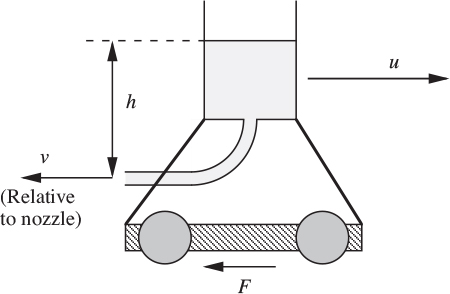
Neglecting fluid friction, use Bernoulli’s equation to derive an expression for v (the exit velocity of the water, relative to the nozzle) in terms of the current value of the height differential h. If the cross-sectional area of the nozzle is A, and the density of water is ρ, give an expression for the mass flow rate m that is leaving the nozzle.
Then perform a momentum balance on the moving jetser, as seen by a stationary observer. Hence, derive an expression for the acceleration du/dt in terms of any or all of h, A, F (the drag force), u, M (the current mass of the vehicle), ρ, and any physical constant(s) that you think are necessary.
38. Force to hold orifice pipe in river—D (C). A thin-walled pipe, of diameter 4 in., is held stationary in a river flowing at 6 ft/s parallel to its axis. The pipe contains a sharp-edged orifice, of diameter 3 in., with a contraction coefficient of 0.60 based on the area. Neglecting entry losses and shear forces on the pipe, and assuming that the orifice is distant from either end of the pipe, calculate the flow rate through the pipe and the force required to hold it in the stream.
39. Froth on sieve tray—D (C). Fig. P2.39 shows the flow pattern on a sieve tray operating at a high liquid flow rate and with a gas that is negligibly absorbed in the liquid. The liquid flows from left to right across the tray; AB is a region of clear liquid where the velocity is uL and the density ρL; the perforations begin at B, and BC is a froth zone, the mean density of the froth being ρF . Show by a momentum balance that the fluid depths in the two regions are related by the equation:
Fig. P2.39. Formation of a froth on a sieve tray.
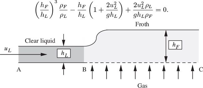
Calculate hF when hL = 0.2 ft, uL = 0.5 ft/s, ρF /ρL = 0.5. Calculate the ratio pL/pF of the pressure increases in the liquid and froth layers.
40. Multiple orifice plates—M (C). What is meant by the pressure recovery behind an orifice plate? Show that the overall pressure drop across an orifice plate, allowing for partial pressure recovery downstream, is kQm, where Q is the volumetric flow rate, m is the mass flow rate, and k is a function of the geometry of the system. Assume that k is constant, but comment on this assumption.
Fig. P2.40. Four orifice plates in a Wheatstone-bridge arrangement.

Four identical orifice plates are connected together in an arrangement analogous to a Wheatstone bridge, as shown in Fig. P2.40. The pump delivers a constant mass flow rate m2 of an incompressible liquid from D to B. Show that, provided m2 is large, the pressure drop between A and C is directly proportional to the liquid mass flow rate m1 in the pipe XY.
What is the critical value of m2, below which this expression for the pressure drop ceases to hold?
41. Pressure recovery in sudden expansion—M (C). Show that at a sudden enlargement in a pipe, the pressure rise is a maximum when the diameter of the larger pipe is ![]() times the fixed diameter of the smaller pipe, and that the rate of energy dissipation is then ρau3/8, in which u is the velocity in the smaller pipe of cross-sectional area a.
times the fixed diameter of the smaller pipe, and that the rate of energy dissipation is then ρau3/8, in which u is the velocity in the smaller pipe of cross-sectional area a.
42. Manifold in reactor base—D (C). Fig. P2.42 shows a manifold MMM for injecting liquid into the base of a reactor. The manifold is formed from a pipe of cross-sectional area A. Liquid enters with velocity v through a pipe P of cross-sectional area a, and leaves uniformly around the circumference of the manifold via a large number of small holes. The rate of recirculation is indicated by the velocity V at section BB just upstream of the injection point. By assuming no loss of energy between sections B and A, but assuming that momentum is conserved from section A to section B, show that, when wall friction is negligible:
Fig. P2.42. Manifold for injecting liquid into the base of a reactor.
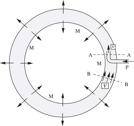
43. Leaking ventilation duct—M (C). A ventilation duct of square cross section operating just above atmospheric pressure has a damaged joint, the longitudinal section being shown in Fig. P2.43. The cross-sectional area open to the atmosphere is 10% of the total cross-sectional area (measured normal to the flow direction).
Fig. P2.43. Ventilation duct with damaged joint.
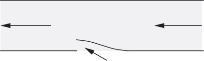
If the velocity upstream of the damaged section is 3 m/s, obtain an expression for the inward leakage rate as a function of the pressure drop along the duct. Neglect pressure drop due to friction. If friction were taken into account, what additional information would be required to solve the problem?
44. Packed-column flooding—M (C). Fig. P2.44 shows an apparatus for investigating the mechanism of flooding in packed columns. A is a vertical cylinder covered by a liquid film that runs down steadily and continuously under gravity. The nozzle B, shown in section, is symmetrical about the centerline of A, and at a typical section X–X the area between the wall of the nozzle and the liquid surface is A = a + bx2.
Fig. P2.44. Apparatus for investigating “flooding.”

Show that if the liquid surface remains cylindrical, and the gas velocity is uniform across any section X–X, the pressure gradient dp/dx in the gas stream will be a maximum at ![]() and will arrest the downward flow of liquid at a gas flow rate Q given by:
and will arrest the downward flow of liquid at a gas flow rate Q given by:
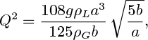
in which ρG and ρL are the gas and liquid densities, respectively.
45. Interpretation of pressure head—M. Analyze the situation in Fig. 2.6(a), and comment critically as to whether the liquid level in the manometer is reasonable as drawn.
46. Velocities and pressures—M. Water flows from point A in the reservoir through a circular channel of varying diameter to its final discharge at point B. Sketch clearly the general trends in the velocity and gauge pressure along the streamline from A to B.
Fig. P2.46. Water flow through varying channel.
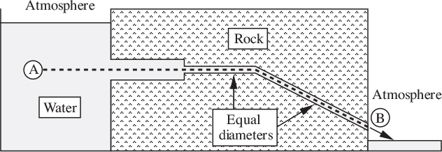
47. True/false. check true or false, as appropriate:
(a) Heat terms are present in the mechanical energy balance, and are absent in Bernoulli’s equation.
T ![]() F
F ![]()
(b) If pure water flows into a tank of brine of constant volume, the concentration of salt in the exit stream decreases exponentially with time.
T ![]() F
F ![]()
(c) Streamlines can cross one another if the fluid has a sufficiently high velocity.
T ![]() F
F ![]()
(d) As gasoline flows steadily upward in a pipe of uniform diameter, its velocity decreases because of the negative influence of gravity.
T ![]() F
F ![]()
(e) In the energy balance or Bernoulli’s equation, the term Δp/ρ has the same units as the square of a velocity.
T ![]() F
F ![]()
(f) If Bernoulli’s equation is divided through by gc, then each term becomes a fluid head, and has the units of length, such as feet or meters.
T ![]() F
F ![]()
(g) Consider an initial (t = 0) liquid level of h = h0 in Fig. 2.7 (tank draining), with a corresponding initial exit flow rate of ![]() The time taken to drain the tank will be the initial volume of liquid in the tank divided by Q0.
The time taken to drain the tank will be the initial volume of liquid in the tank divided by Q0.
T ![]() F
F ![]()
(h) A Pitot tube works on the principle of converting kinetic energy into potential energy.
T ![]() F
F ![]()
(i) As fluid flows through an orifice plate to the location of the vena contracta, its pressure will rise, because it is going faster there.
T ![]() F
F ![]()
(j) If a value for the frictional dissipation term F is known for an orifice plate in a horizontal pipe, it can also be applied to situations that are not necessarily horizontal.
T ![]() F
F ![]()
(k) If a mercury manometer connected across an orifice plate with kerosene flowing of density ρk through it registers a difference of Δh in levels, the corresponding pressure drop is p1 − p2 = ρHggΔh.
T ![]() F
F ![]()
(l) A stream of mass flow rate m and velocity u convects momentum at a rate mu2.
T ![]() F
F ![]()
(m) At any instant, the rate of increase of momentum of a liquid-fueled rocket is Mdv/dt, where M is the current mass of the rocket and v is its velocity.
T ![]() F
F ![]()
(n) The thrust of a jet engine is m(v − u), where m is the mass flow rate through the engine, v is the velocity of the exhaust relative to the engine, and u is the velocity of the craft on which the engine is mounted.
T ![]() F
F ![]()
(o) There is always a pressure decrease across a sudden expansion in a pipeline.
T ![]() F
F ![]()
(p) A hydraulic jump is irreversible, and can occur only when a relatively deep stream of liquid suddenly becomes a relatively shallow stream.
T ![]() F
F ![]()
(q) The momentum of a baseball decreases between the mound and plate because of gravitational forces.
T ![]() F
F ![]()
(r) A boat, traveling forwards at a velocity u on a lake, has a pump on board that takes water from the lake and ejects it to the rear at a velocity v relative to the boat. The velocity of the water as seen by an observer on the shore is v − u in the forwards direction.
T ![]() F
F ![]()
(s) After the fluid downstream of an orifice plate has reestablished its flow pattern, it will return to the same pressure that it had upstream of the orifice plate.
T ![]() F
F ![]()
(t) Bernoulli’s equation (with w = F = 0) holds across a sudden expansion in a pipe.
T ![]() F
F ![]()
(u) A momentum balance can be used to determine the frictional dissipation term, F, for a sudden expansion in a pipeline.
T ![]() F
F ![]()
(v) A pirouetting (spinning) ice skater, with her arms outstretched, rotates faster when she brings her hands together above her head mainly because of the reduced air drag.
T ![]() F
F ![]()