
Chapter 9. Turbulent Flow
9.1 Introduction
TURBULENT fluid motion has been aptly described as “an irregular condition of flow in which the various quantities show a random variation with time and space coordinates, so that statistically distinct average values can be discerned.”1
1 J.O. Hinze, Turbulence—an Introduction to Its Mechanism and Theory, McGraw-Hill, New York, 1959.
A thorough understanding of turbulence has not been achieved to date, and may never be attained in the foreseeable future. For this reason, the subject is sometimes neglected in introductory fluid mechanics courses. But this should not be the case, and we should not be discouraged from trying to learn something about it, because—as nice as the solutions for laminar flow are—turbulence is the more normal state of affairs in fluid flow. To be sure, there are important cases in which the flow is indeed laminar, and at least two fields come readily to mind: polymer processing (typically with high viscosities) and microfluidics (with very tiny channel dimensions). However, there are countless other situations involving turbulence, such as gas flow in long-distance pipelines, liquid flow in heat exchangers, blood flow in the heart, combustion of gases, many industrial reactors, and so on.
We cannot resist the temptation of reproducing the famous quotation recalled by Parviz Moin and John Kim2: “The difficulty with turbulence was wittily expressed in 1932 by the British physicist Horace Lamb, who, in an address to the British Association for the Advancement of Science, reportedly said, ‘I am an old man now, and when I die and go to heaven there are two matters on which I hope for enlightenment. One is quantum electrodynamics, and the other is the turbulent motion of fluids. And about the former I am rather optimistic.’”
2 Tackling Turbulence with Supercomputers, http://turb.seas.ucla.edu/˜jkim/sciam/turbulence.html
In this chapter, our goals will be:
1. To gain some understanding of turbulent flow in pipes, channels, and jets.
2. To investigate the analogies between the turbulent transport of momentum and thermal energy.
3. To learn more about how computational fluid dynamics (CFD) is starting to allow us to tackle turbulence in more complicated situations by the numerical solution of certain equations of motion. In particular, we shall study the k–ε method, which deals with the production and dissipation of turbulent kinetic energy. Although the method has some limitations, its relatively easy implementation (by Fluent and COMSOL, for example) does at least lead to plausible and useful results in many instances.
The reader will already know that the Reynolds number, being a measure of the relative importance of inertial effects to viscous effects, is an important factor in determining whether turbulence is likely to occur or not. At low Reynolds numbers, viscous effects dominate, and will dampen out any small perturbations in the flow. But at higher Reynolds numbers this is no longer the case, and the predominance of the nonlinear inertial terms in the Navier-Stokes equations will lead to an amplification of small perturbations. The consequence is that in addition to the general trend of flow there will be superimposed eddies, being regions that are typically rotating and hence have vorticity, behaving as little whirlpools. For pipe flow, the eddies that are initially formed at the expense of pressure energy are of a size that is the same order of magnitude as the pipe diameter. But these larger eddies are themselves unstable and break down into progressively smaller eddies, the general scheme being shown in simplified form in Fig. 9.1.
Fig. 9.1. Simplified overall picture of the cascade process.

Although the energy per eddy is highest for the large eddies, there are so many more of the smaller eddies that the total amount of mechanical energy passed down the chain or cascade remains essentially constant. But the process eventually terminates, when the eddies become so small that their velocity variations occur over such short distances (known as the Kolmorogov limit) that the resulting high-velocity gradients cause viscosity to kick in and convert the mechanical energy into heat.
Mathieu and Scott, authors of an excellent and comprehensive introduction to turbulence, state that the energy cascade from large to small turbulent eddies was first postulated by Lewis F. Richardson.3 And it was in Richardson’s publication that he summarized his beliefs in the famous lines:
3 J. Mathieu and J. Scott, An Introduction to Turbulent Flow, Cambridge University Press, 2000, p. 61. The following reference is given: L.F. Richardson, Weather Prediction by Numerical Process, Cambridge University Press, 1922.
Big whorls have little whorls, Which feed on their velocity; And little whorls have lesser whorls, And so on to viscosity.
Although turbulence is more likely to occur at the higher Reynolds numbers, it is also promoted by the shearing action of a solid surface, and tends to be enhanced in the wake downstream of an object such as an airplane wing or golf ball. But note that at moderate Reynolds numbers it is possible to have a laminar flow that is unstable but cannot be classified as turbulent. The last example in Chapter 13 shows how CFD can simulate (with considerable accuracy) the flow past a cylinder at a moderate Reynolds number of 100. In that event, the instability of the laminar flow causes vortices to be shed alternately from opposite sides of the cylinder, forming a Kármán vortex street. However, the vortices are generated in a regular pattern and therefore do not satisfy the criterion of randomness or chaotic behavior that characterizes turbulence.
Generally, turbulent flow occurs at sufficiently high values of the Reynolds number, at conditions under which laminar flow becomes unstable and the velocities and pressure no longer have constant or smoothly varying values. For pipe flow, the general picture is that relatively large rotational eddies are formed in the region of high shear near the wall, and that these degenerate into progressively smaller eddies, in which the energy is dissipated into heat by the action of viscosity.
To proceed, we recognize that turbulence is inherently a three-dimensional phenomenon, and at any point P there will be fluctuations in time of the three velocity components shown in Fig. 9.2.4 It is first necessary to introduce the concept of a time-averaged quantity, denoted by an overbar, defined as the mean value of that quantity over a time period T that is very large in comparison with the time scale of the individual fluctuations. Thus, ![]() is the time-averaged value of the x velocity component, vx.
is the time-averaged value of the x velocity component, vx.
4 Nevertheless, useful information about turbulence can still be obtained in situations that have just two coordinates of primary interest, such as r and z that occur in pipe flow.
Fig. 9.2. Fluctuating velocity components.
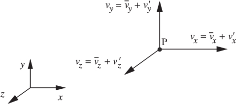
Then, at any point in space, we can think of the three individual velocity components and the pressure at any instant of time as being given by:
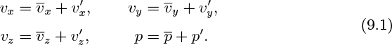
Here, ![]() etc. denote fluctuations from the mean values, and which may change very rapidly—in a matter of milliseconds, as shown in Fig. 9.3; in such event, a value of T equal to a few seconds would be appropriate for the time averaging just described. This chapter generally deals with flows such as those in pipes and jets that are steady in the mean—that is, these time-averaged quantities do not vary with time; in other situations, they may fluctuate slowly with time.
etc. denote fluctuations from the mean values, and which may change very rapidly—in a matter of milliseconds, as shown in Fig. 9.3; in such event, a value of T equal to a few seconds would be appropriate for the time averaging just described. This chapter generally deals with flows such as those in pipes and jets that are steady in the mean—that is, these time-averaged quantities do not vary with time; in other situations, they may fluctuate slowly with time.
Fig. 9.3. Variation of instantaneous velocity vx with time t. The fluctuations typically occur over a period of a few milliseconds.
If the fluctuations shown in Fig. 9.3 could be examined under a succession of increasingly powerful magnifying glasses, the fluctuations would not be smooth and a certain amount of “fuzziness” would be seen, corresponding to the continuously smaller eddies in the overall energy cascade. However, a limit would eventually be reached (the Kolmorogov limit) when the length scale is sufficiently small that the fluctuations do finally look smooth.
By definition, the time averages of the fluctuations are zero, since—on the average—they are equally likely to be above the mean or to fall below it:
Therefore, the time averages of the mean quantities are the mean quantities themselves; for example:
The intensity of the turbulence is typically in the range given by:

in which the root-mean-square of the fluctuating velocity component is defined as:
Time-averaged continuity equation
From Eqn. (5.52), the continuity equation with constant density is:

Now substitute the instantaneous velocity components from Eqn. (9.1) and time average the entire equation. A representative term, and its subsequent rearrangement, is:

Observe the four intermediate steps involved:
1. The time average of the partial derivative of a quantity equals the partial derivative of the time average of that quantity.
2. The time average of the sum of two quantities equals the sum of their individual time averages.
3. From Eqn. (9.3), the time average of a mean quantity, (vx) in this case, is that mean quantity itself.
4. From Eqn. (9.2), the time average of a fluctuating component is zero.
Time averaging the other derivatives as well yields the time-averaged continuity equation:

which is identical with the original continuity equation except that time-averaged velocities have replaced the instantaneous velocities.
Time-averaged momentum balances
(The reader who is not interested in tedious derivations, or doesn’t have time for them, can skip immediately from Eqn. (9.9) to the final result, Eqn. (9.13).) The x momentum balance (for example) in terms of the viscous stress components is, from Eqn. (5.72):

We again substitute the instantaneous velocity components from Eqn. (9.1) and time average the resulting equation to give the time-averaged x momentum balance. However, the following intermediate steps, relating to the nonlinear terms on the left-hand side, are useful. First note that these terms can be rewritten, with the aid of the continuity equation, (9.6), as:

Eqn. (9.10) may also be proved by noting that the left-hand side can be written as v · ∇vx. The vector identity ∇ · vxv = vx∇ · v + v · ∇vx = v · ∇vx for an incompressible fluid [see Eqn. (5.24)] leads directly to the right-hand side of Eqn. (9.10).
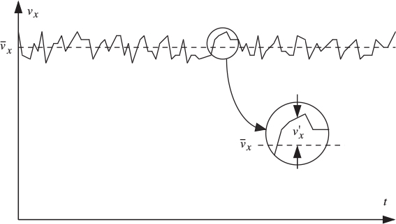
Now substitute the instantaneous velocity components from Eqn. (9.1) into the right-hand side of Eqn. (9.10) and time-average the result. We now have to deal with the time averages of quantities such as ![]() . Time-averaged in the usual way, these terms become:
. Time-averaged in the usual way, these terms become:
which, with the aid of time-averaged continuity equation, (9.8), may be rephrased as:

By replacing the time-averaged nonlinear terms on the left-hand side of Eqn. (9.9) with those from Eqn. (9.12), the complete time-averaged x momentum balance becomes:

Here, the time-averaged viscous shear stresses, such as ![]() , are based in the usual way by Newton’s law on the time-averaged velocity profiles. Observe that the time-averaged momentum balance is the same as the original (instantaneous) momentum balance, except that:
, are based in the usual way by Newton’s law on the time-averaged velocity profiles. Observe that the time-averaged momentum balance is the same as the original (instantaneous) momentum balance, except that:
1. Time-averaged values have replaced the original instantaneous values.
2. Additional stresses, known as the Reynolds stresses, have now appeared on the right-hand side, and represent the transport of momentum due to turbulent velocity fluctuations. A physical interpretation of these stresses will be given in the next section. Calculations for all but the lowest intensities of turbulence show that a Reynolds stress such as ![]() (the superscript t denotes turbulence) is very much larger than its viscous or molecular counterpart
(the superscript t denotes turbulence) is very much larger than its viscous or molecular counterpart ![]() (except very close to a wall), so the latter can be ignored in most situations.
(except very close to a wall), so the latter can be ignored in most situations.
Time-averaged y and z momentum balances give similar results.
A short example will give a better understanding of a term such as ![]() that appears in a typical Reynolds stress. For simplicity, consider a hypothetical situation in which only “quantum” values of the fluctuating components are permitted, and only allow each of
that appears in a typical Reynolds stress. For simplicity, consider a hypothetical situation in which only “quantum” values of the fluctuating components are permitted, and only allow each of ![]() and
and ![]() to have values of either −1 (low) or 1 (high). Investigate the possible values for
to have values of either −1 (low) or 1 (high). Investigate the possible values for ![]() . (A more elaborate investigation would involve a statistical analysis of a continuous distribution of velocities, but the main thrust would not differ significantly from that in the present, more elementary, treatment.)
. (A more elaborate investigation would involve a statistical analysis of a continuous distribution of velocities, but the main thrust would not differ significantly from that in the present, more elementary, treatment.)
Solution
Table 9.1 shows three possibilities, two in which the fluctuations ![]() and
and ![]() are correlated, and the other in which they are independent of each other.
are correlated, and the other in which they are independent of each other.
Table 9.1. Possible Values for Velocity Fluctuations
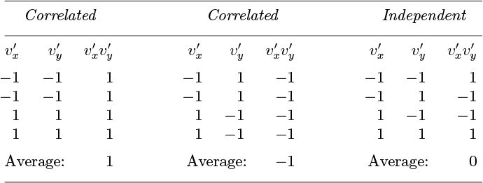
Observe that in the first two cases, the time-averaged values ![]() of the product are nonzero, being (1+1+1+1)/4 = 1 when the individual fluctuations move in concert with each other (high values occur together, and so do low values), and −1 when they are opposed to each other (a high value of one occurs with a low value of the other). In the third example, when the fluctuations are quite independent of each other, the time-averaged value
of the product are nonzero, being (1+1+1+1)/4 = 1 when the individual fluctuations move in concert with each other (high values occur together, and so do low values), and −1 when they are opposed to each other (a high value of one occurs with a low value of the other). In the third example, when the fluctuations are quite independent of each other, the time-averaged value ![]() is zero. The Reynolds stresses are therefore only nonzero when there is a certain degree of correlation between the fluctuations in the different coordinate directions. Such correlations do tend to occur in turbulent flow.
is zero. The Reynolds stresses are therefore only nonzero when there is a certain degree of correlation between the fluctuations in the different coordinate directions. Such correlations do tend to occur in turbulent flow.
9.2 Physical Interpretation of the Reynolds Stresses
The Reynolds stresses may also be understood by considering the fragments of fluid, or “eddies,” that suddenly jump across a unit area of the plane X–X due to turbulent motion, as shown in Fig. 9.4. Here, we are considering two-dimensional flow with ![]() and
and ![]() (no overall motion in the y direction).
(no overall motion in the y direction).
Fig. 9.4. Motion of an eddy upward across the plane X–X.

Observe that the instantaneous rate of transfer of x momentum in the y direction, from below X–X to above it, is, per unit area:
This result is obtained by noting that the x momentum of the eddy is ![]() per unit volume, and that the volume flux in the y direction is simply the velocity
per unit volume, and that the volume flux in the y direction is simply the velocity ![]() . Hence, considering fluid crossing X–X from either above or below, at all possible velocities, the time-averaged rate of transfer of x momentum in the y direction, is, per unit area:
. Hence, considering fluid crossing X–X from either above or below, at all possible velocities, the time-averaged rate of transfer of x momentum in the y direction, is, per unit area:
The conventional direction for shear stress is expressed in Fig. 5.12 and also by the box in Fig. 9.4, so we need the rate of transfer of x momentum from above X–X to below it—that is, in the negative y direction; the resulting shear stress due to turbulent fluctuations must therefore include a negative sign:
9.3 Mixing-Length Theory
Unfortunately, there is no universal law whereby the turbulent shear stress of Eqn. (9.16) can be predicted, and it is necessary to resort to a semitheoretical approach in conjunction with experimental observations.
Consider the rate of transport ![]() of x momentum, whose time-averaged value is
of x momentum, whose time-averaged value is ![]() per unit volume, across the representative plane X–X shown in Fig. 9.5. Suppose that this momentum is transferred from one plane to another by a series of eddies that—on the average—move a distance λ in the y direction and then suddenly lose their identity and mix completely with the surrounding fluid.
per unit volume, across the representative plane X–X shown in Fig. 9.5. Suppose that this momentum is transferred from one plane to another by a series of eddies that—on the average—move a distance λ in the y direction and then suddenly lose their identity and mix completely with the surrounding fluid.
Fig. 9.5. Transport of x momentum across the plane X–X.
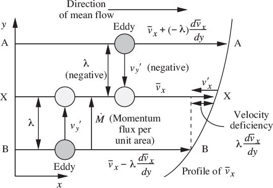
In more detail, there will be x momentum transport across unit area of X–X by elements of fluid coming with velocities ![]() from planes A–A and B–B at distances λ from above and below X–X. Since
from planes A–A and B–B at distances λ from above and below X–X. Since ![]() and λ have the same sign for the same eddy (both are positive for the eddy from B–B and both are negative for the eddy from A–A), the same equation holds in either direction. Thus, we only need to consider the eddy traveling upward from B–B.
and λ have the same sign for the same eddy (both are positive for the eddy from B–B and both are negative for the eddy from A–A), the same equation holds in either direction. Thus, we only need to consider the eddy traveling upward from B–B.
Also note from Fig. 9.5 that if the value of momentum is ![]() at the midplane X–X, it will be less than this value at the lower plane B–B; assuming that the gradient
at the midplane X–X, it will be less than this value at the lower plane B–B; assuming that the gradient ![]() is approximately constant, the deficiency is
is approximately constant, the deficiency is ![]() . A total derivative is used, it being assumed that the time-averaged velocity profile is fully established.
. A total derivative is used, it being assumed that the time-averaged velocity profile is fully established.
Per unit area, the rate of turbulent transfer of x momentum from B–B across X–X is:

As noted, Eqn. (9.17) holds equally well for the transfer in either direction.
The time-averaged net upward rate of transport, in the y direction, is therefore:

But, by definition, ![]() . Also assume that the gradient
. Also assume that the gradient ![]() is constant over the region, giving:
is constant over the region, giving:

in which the time-averaged quantity ![]() is called the eddy kinematic viscosity; the subscript T emphasizes a turbulent quantity.
is called the eddy kinematic viscosity; the subscript T emphasizes a turbulent quantity.
To proceed further, we must transform ![]() into something more tractable. To start, it can be reexpressed as the product of the RMS (root-mean-square) values of its individual components, multiplied by a correlation-coefficient R:
into something more tractable. To start, it can be reexpressed as the product of the RMS (root-mean-square) values of its individual components, multiplied by a correlation-coefficient R:
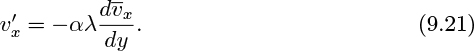
Also consider the mechanism that causes a turbulent fluctuation ![]() in the x velocity component at the central plane X–X, noting that the curve in Fig. 9.5 represents the time-averaged x velocity,
in the x velocity component at the central plane X–X, noting that the curve in Fig. 9.5 represents the time-averaged x velocity, ![]() . Clearly, the x velocity is lower at the plane B–B than it is at the midplane X–X, by an amount
. Clearly, the x velocity is lower at the plane B–B than it is at the midplane X–X, by an amount ![]() , also known as the velocity “deficiency.” Thus, an eddy suddenly moving from B–B to X–X will also have an x momentum deficiency, and will impart a negative “kick” to the x velocity at the plane X–X. The resulting fluctuation will be proportional to the velocity deficiency. Approximately, if α is a constant:
, also known as the velocity “deficiency.” Thus, an eddy suddenly moving from B–B to X–X will also have an x momentum deficiency, and will impart a negative “kick” to the x velocity at the plane X–X. The resulting fluctuation will be proportional to the velocity deficiency. Approximately, if α is a constant:
The same result will hold for an eddy traveling downward from A–A to X–X, for in that case λ is negative and the fluctuation is positive. In terms of RMS values:

Experimentally, ![]() tends to be proportional to
tends to be proportional to ![]() —that is, the velocity fluctuations are generally correlated with each other:
—that is, the velocity fluctuations are generally correlated with each other:

Here, the coefficient β would be unity for isotropic turbulence, in which the intensity of turbulence is uniform in all directions.
From Eqns. (9.19), (9.20), and (9.23):
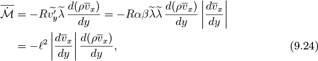
a result obtained by Prandtl in 1925, in which:
is the Prandtl mixing length.
Also note that the eddy kinematic viscosity can be expressed in terms of the Prandtl mixing length and the velocity gradient:

Similar analyses can be performed for the rates of turbulent transport of heat and mass (the last typically for a single chemical species when others are present). All results are summarized in Table 9.2, in which cp denotes specific heat, and ![]() and c are the time-averaged temperature and species concentration, respectively. Since the shear stress conventionally denotes a transfer of momentum in the negative y direction (see Section 9.2), there is a minus sign preceding
and c are the time-averaged temperature and species concentration, respectively. Since the shear stress conventionally denotes a transfer of momentum in the negative y direction (see Section 9.2), there is a minus sign preceding ![]() ; however, heat and mass transfer are conventionally taken in the positive y direction so no minus sign is needed in these cases. Partial derivatives are used for the temperature and concentration gradients because in a heat exchanger or tubular reactor
; however, heat and mass transfer are conventionally taken in the positive y direction so no minus sign is needed in these cases. Partial derivatives are used for the temperature and concentration gradients because in a heat exchanger or tubular reactor ![]() and c would almost certainly vary both in the transverse (y) direction and in the direction of the main flow.
and c would almost certainly vary both in the transverse (y) direction and in the direction of the main flow.
Table 9.2. Summary of Relations for Turbulent Transport
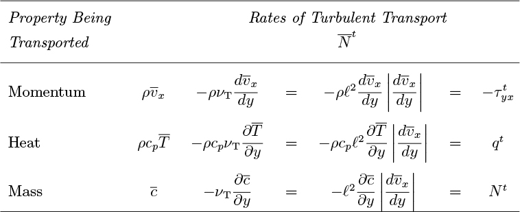
Table 9.2 assumes that the eddy thermal diffusivity αT and the eddy diffusivity DT are the same as the eddy kinematic viscosity νT, which is true only as a first approximation. Section 9.13 explores the relation between turbulent heat and momentum transport in more detail.
9.4 Determination of Eddy Kinematic Viscosity and Mixing Length
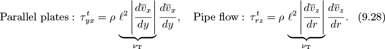
Note that the eddy kinematic viscosity can be determined fairly readily as a function of position. For flow between parallel plates and for pipe flow, momentum balances on the elements shown in Fig. 9.6 give:

Fig. 9.6. Shear stresses for (a) parallel plates, (b) pipe.

where y is here measured from the centerline. Here, the typically very small laminar or viscous shear stresses ![]() and
and ![]() have been ignored, but could easily be retained if high accuracy is needed, especially near the walls. Since pressure drops and hence pressure gradients can easily be measured, the turbulent shear stress
have been ignored, but could easily be retained if high accuracy is needed, especially near the walls. Since pressure drops and hence pressure gradients can easily be measured, the turbulent shear stress ![]() or
or ![]() can be deduced at any location. Velocity profiles and hence velocity gradients such as
can be deduced at any location. Velocity profiles and hence velocity gradients such as ![]() can also be measured by means of a Pitot tube or laser-Doppler velocimetry. The mixing lengthℓ and the eddy kinematic viscosity νT are then obtained from:
can also be measured by means of a Pitot tube or laser-Doppler velocimetry. The mixing lengthℓ and the eddy kinematic viscosity νT are then obtained from:
For both smooth and rough pipes, experiments show5 that the ratio of the mixing length to the pipe radius is given very accurately by:
5 See Eqn. (20.18) in H. Schlichting, Boundary Layer Theory, Pergamon Press, New York, 1955.
which is plotted in Fig. 9.7. Note that as the wall is approached, l =0.4y, which is the simplified result used in the Prandtl hypothesis. However, at greater distances from the wall, the eddies have more freedom to travel and a maximum value is reached at the centerline.
Fig. 9.7. Variation of dimensionless mixing length with location.

Further, the experiments of Nikuradse in smooth pipes show the variation of the dimensionless eddy kinematic viscosity is given approximately by:

and very accurately by:

in which there is no term in (y/a)4. The accurate correlation of Eqn. (9.31) is plotted in Fig. 9.8.
Fig. 9.8. Variation of dimensionless eddy viscosity with location.

Recall from Eqn. (9.28) that the eddy viscosity is given by the product of the square of the mixing length and the magnitude of the velocity gradient:

The shape of the curve in Fig. 9.8 is now easily explained. Moving away from the wall, as l increases, the eddy viscosity also increases and indeed reaches a maximum halfway to the centerline. Thereafter, the declining velocity gradient is the dominant factor, and the eddy viscosity falls significantly (but not quite to zero) as the centerline is reached.
9.5 Velocity Profiles Based on Mixing-Length Theory
The Prandtl hypothesis
Consider pipe flow, with axial coordinate z. The simplest model—that of Prandtl—assumes a direct proportionality between the mixing lengthℓ and the distance y from the wall, the argument being that the eddies have more freedom of motion the further they are away from the wall. Also assume a constant shear stress ![]() , equal to its value τw at the wall, which is strictly only true for a small interval near the wall:
, equal to its value τw at the wall, which is strictly only true for a small interval near the wall:
Actually, Eqns. (9.33) and (9.34) are overestimates for both ℓ and ![]() ; fortuitously, both overestimates will tend to cancel each other and give an excellent result for the turbulent velocity profile! Note that for the moment it is more expedient to work with y than r as the transverse coordinate, hence the notation
; fortuitously, both overestimates will tend to cancel each other and give an excellent result for the turbulent velocity profile! Note that for the moment it is more expedient to work with y than r as the transverse coordinate, hence the notation ![]() .
.
Mixing-length theory also gave the formula:

in which ![]() is recognized as positive, since the time-averaged velocity increases as the distance from the wall increases.6 From the above:
is recognized as positive, since the time-averaged velocity increases as the distance from the wall increases.6 From the above:
6 For the rest of the chapter, the designation “time-averaged” will be dropped, it being assumed that any quantity with an overline is so denoted.

which integrates to:

in which c is a constant of integration. Experimentally, it is found, perhaps rather surprisingly, that the velocity profile of Eqn. (9.37) also holds in the central region of a pipe, with k . =0.4. Since ln y is fairly insensitive to changes in y, Eqn. (9.34) predicts a fairly “flat” turbulent velocity profile, in accordance with experimental observation.
Note that the logarithmic law cannot possibly hold very close to the wall, because as y tends to zero, it gives an ever-increasing negative velocity, and an ever-increasing velocity gradient.
Von Kármán proposed that the mixing length should be proportional to the ratio of the first two derivatives of the velocity:
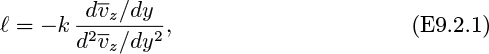
in which k is a dimensionless constant. Investigate the merits of this hypothesis and compare its predictions for the velocity profile with that of Prandtl.
Solution
The Prandtl hypothesis expressed the mixing length in terms of the distance from the wall. But turbulence can occur in a region well away from a wall (in the upper atmosphere, to take an extreme example), where the impact of the wall is small—that is, where there is no obvious length scale on which to base ℓ.
First, observe that the ratio of the first and second derivatives of the velocity in Eqn. (E9.2.1) has indeed the desired dimensions of length. Thus, an obvious advantage of the von Kármán hypothesis is that it gives the mixing length in terms of the local behavior of the velocity profile, rather than relying on the presence of a wall for the length scale.
From Eqns. (9.32) and (E9.2.1), again assuming near the wall that ![]() :
:

which integrates to:
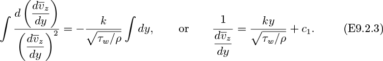
The constant of integration c1 disappears if we assume that the velocity gradient ![]() becomes very steep and approaches infinity at the wall, where y = 0. A second integration gives:
becomes very steep and approaches infinity at the wall, where y = 0. A second integration gives:
which is identical with the result from Prandtl’s hypothesis.
A disadvantage of the von Kármán hypothesis is that it fails if ![]() is zero, a situation that can quite easily occur—for example, at the inflection points in the velocity profiles of the turbulent jets discussed in Section 9.13.
is zero, a situation that can quite easily occur—for example, at the inflection points in the velocity profiles of the turbulent jets discussed in Section 9.13.
Suppose that the more realistic shear-stress distribution for pipe flow, ![]() , where a is the pipe radius and r is the distance from the centerline, is used in conjunction with the mixing-length theory of Eqn. (9.29) and the von Kármán hypothesis of Example 9.2. A double integration, noting an infinite velocity gradient at the wall to determine one constant of integration, gives:
, where a is the pipe radius and r is the distance from the centerline, is used in conjunction with the mixing-length theory of Eqn. (9.29) and the von Kármán hypothesis of Example 9.2. A double integration, noting an infinite velocity gradient at the wall to determine one constant of integration, gives:

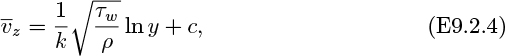
in which ![]() is the centerline velocity. For reasons already given, this seemingly more sophisticated result is not as accurate as the simpler law of Eqn. (9.34).
is the centerline velocity. For reasons already given, this seemingly more sophisticated result is not as accurate as the simpler law of Eqn. (9.34).
9.6 The Universal Velocity Profile for Smooth Pipes
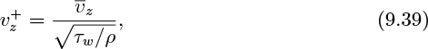
The logarithmic law of Eqn. (9.37) is now rephrased in terms of dimensionless variables. First, define a dimensionless distance from the wall, y+, and a dimensionless velocity, ![]() , by:
, by:
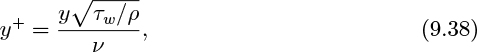
in which ν is the kinematic viscosity. Equation (9.37) can then be rewritten as:

or:
in which A is a constant of integration and B = 1/k. The quantity ![]() known as the friction velocity and is given the symbol
known as the friction velocity and is given the symbol ![]() .
.
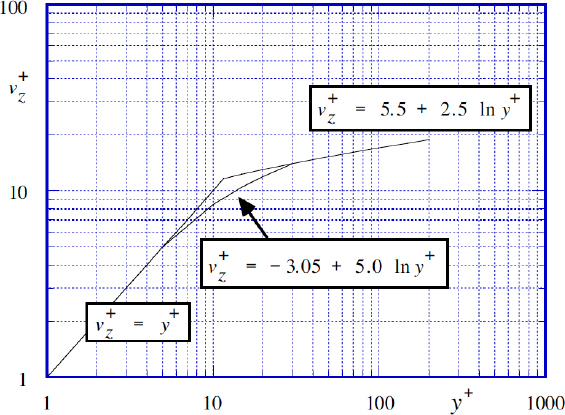
Equation (9.41) is known as the universal velocity profile, because it gives exceptionally good agreement with experimental velocities over a very wide range of Reynolds number for smooth pipes.7 Experimentally, the constants are A =5.5 and B =2.5, giving:
7 For example, see the velocities displayed on page 405 of Schlichting, op. cit.
Of course, Eqn. (9.42) does not hold very close to the wall, where, by integration of ![]() in the laminar sublayer:
in the laminar sublayer:
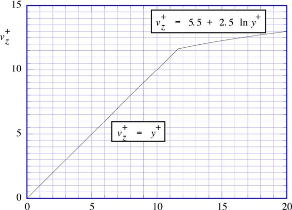
As shown in Fig. 9.9, the turbulent and laminar velocity profiles of Eqns. (9.42) and (9.43) intersect at y+ =11.63.
Fig. 9.9. The universal velocity profile.
To represent the experimental data of Nikuradse even better, particularly in a buffer region between the laminar sublayer and the fully developed turbulent core, von Kármán divided the complete velocity profile into three regions:
Laminar sublayer:
Buffer region:
Turbulent core:
The following velocity profile, based on a theory of Sleicher and discussed further in Problem 9.10, also gives an excellent fit of turbulent velocities in the laminar sublayer and buffer regions:
9.7 Friction Factor in Terms of Reynolds Number for Smooth Pipes
For the purposes of obtaining the total flow rate, and hence the mean velocity, the logarithmic profile v+z = A + B ln y+ can be assumed to hold over the whole pipe, because the laminar sublayer is so thin and contributes virtually nothing to the flow. Thus, the mean z velocity is:

which can be shown by integration (see Example 9.3) to equal:
Thus, for the profile with A =5.5 and B =2.5 in Eqn. (9.46):
the integration gives:

Recall the Fanning friction factor, defined as:
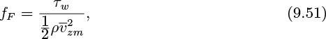
in which ![]() has the same meaning as um used in Chapter 3. It follows from Eqns. (9.50) and (9.51) that—based on the universal velocity profile—the friction factor and Reynolds number are related by:
has the same meaning as um used in Chapter 3. It follows from Eqns. (9.50) and (9.51) that—based on the universal velocity profile—the friction factor and Reynolds number are related by:

Experimentally, a law similar to Eqn. (9.52),

agrees with experiment for smooth pipes over a very wide range of Re (from 5×10³ up to at least 3.4 × 10⁶ and probably beyond).
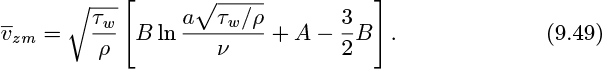
For the velocity profile given by ![]() , prove the formula for the mean velocity given in Eqn. (9.49).
, prove the formula for the mean velocity given in Eqn. (9.49).
Solution
Noting the definitions of the dimensionless velocity and distance from the wall, the given velocity profile can be rewritten as:

The mean velocity vzm is therefore:

Noting that insertion ln ydy = y ln y − y and y ln ydy =(y2/2) ln y − (y2/4), integration, of limits, and collection of terms gives:

which is the desired result.
9.8 Thickness of the Laminar Sublayer
The thickness of the laminar sublayer will be diminished as the Reynolds number increases, because the more vigorous turbulent eddies approach the wall more closely. For simplicity in the following analysis, ignore the presence of the buffer region, and assume just a “two-piece” model, which is needed for the Prandtl-Taylor analogy of Section 9.13.
Start with the known velocity profiles in the two regions, which are also shown in Fig. 9.10:
Laminar sublayer:
Turbulent core:
Fig. 9.10. Velocity profiles in the laminar sublayer and part of the turbulent core.
The thickness δ of the laminar sublayer is now determined as a function of the Reynolds number. At the junction between the two regions, the velocities must match each other:
That is, the thickness δ of the laminar sublayer and the velocity vzδ at the laminar sublayer/turbulent core junction are:

That is,

Although fF is given by Eqn. (9.53), a somewhat simpler relationship—of admittedly more limited range (Re < 105)—is the Blasius law:
From Eqns. (9.56) and (9.57), the ratio of the laminar sublayer thickness to the pipe diameter is:
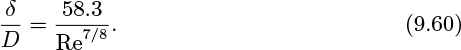
For a slightly different velocity-profile equation, the one-seventh power law,
in which vzc is the centerline velocity, the result is only marginally different:

If representative values for the Reynolds numbers are substituted into the above equations, they will show that:
1. The laminar sublayer is an extremely thin region, across which the velocity builds up to a significant portion of its centerline value.
2. The thickness of the laminar sublayer decreases almost in direct proportion to the value of the Reynolds number.
If a three-piece velocity profile is considered, as in Fig. 9.9, then the outer edge of the laminar sublayer occurs at y+ = 5, and the ratio δ/D becomes:
9.9 Velocity Profiles and Friction Factor for Rough Pipe
In turbulent flow, the wall irregularities may or may not project through the laminar sublayer. Depending on the extent of the wall roughness ε as discussed in Section 3.4, three regimes may be delineated—each supported by experiment— with differing dependencies for the friction factor:
Hydraulically smooth pipe:
Transition state:
Completely rough pipe:
The turbulent velocity profiles in all three regions can be represented by:
in which the values of B and the corresponding velocity profiles, except for the transition region, are:
Hydraulically smooth pipe:

Completely rough pipe:

For smooth pipe, we have already noted that Eqn. (9.68) is the universal velocity profile. For completely rough pipe, Eqn. (9.69) is independent of the pipe radius, and its validity is completely substantiated by experiments over a very wide range of roughness ratios ε/D.8
8 See page 420 of Schlichting, op. cit., for experimental evidence.
The Colebrook and White equation is consistent with the above observations and represents the variation of the Fanning friction factor with the relative roughness and the Reynolds number over a very wide range of roughnesses and (turbu-lent) Reynolds numbers:

9.10 Blasius-Type Law and the Power-Law Velocity Profile
Experimentally, for smooth pipe, provided that the Reynolds number is no larger than 105:
More generally, for other values of the Reynolds number:

But, by definition of the friction factor:
From Eqns. (9.71) and (9.72), elimination of the friction factor gives:
Now take a power-law velocity profile of the general form:
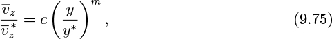
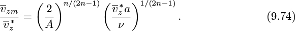
which gives, after suitable integration:

By equating exponents on the Reynolds number in Eqns. (9.74) and (9.76):
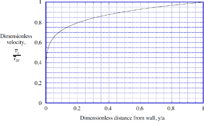
For example, if n = 4, then m = 1/7, which is a familiar result, and is shown in Fig. 9.11.
Fig. 9.11. One-seventh power-law velocity profile.
There is also another relation between c in the velocity profile and A in the expression for fF. Determination of either of these experimentally shows that c =8.74, that is:

Solving for ![]() :
:

which can now be back-substituted into the expression for the wall shear stress, Eqn. (9.73):

This last expression is analogous to the Blasius law, but now contains the velocity ![]() at a definite distance y from the wall. Note that it was used for finding the thickness of the turbulent boundary layer in Section 8.5.
at a definite distance y from the wall. Note that it was used for finding the thickness of the turbulent boundary layer in Section 8.5.
9.11 A Correlation for the Reynolds Stresses
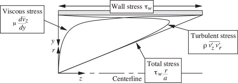
Fig. 9.12 shows how the total shear stress for flow in a pipe is the sum of the viscous and turbulent contributions. Note that the turbulent or Reynolds stress term dominates over most of the region, but declines sharply to zero at the wall, whereas that the viscous term is the main effect very close to the wall.
Fig. 9.12. A graph showing how the total shear stress is the sum of the viscous and turbulent stresses. All quantities shown are positive. (Not to scale.)
In recent years, S.W. Churchill and S.C. Zajic have proposed a valuable alternative to mixing length and eddy viscosity correlations for flow in simple geometries, and their approach concentrates instead on the Reynolds stress term.9
9 S.W. Churchill and S.C. Zajic, “Prediction of fully developed turbulent convection with minimal explicit empiricism,” American Institute of chemical Engineers Journal, Vol. 48, No. 5 (May 2002), p. 927.
For pipe flow the starting point is the time-averaged z momentum equation, similar to Eqn. (9.13). With the usual simplifications, there results:

The wall shear stress τw, which is traditionally taken to be a positive quantity, is related to the pressure gradient by Eqn. (9.27):
Thus, separation of variables and integration of Eqn. (9.81) gives:

Since both integrands are zero at the lower limit, the result is:
But the viscous stress is given by ![]() , in which y = a − r is the distance from the wall, giving:
, in which y = a − r is the distance from the wall, giving:
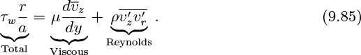
Fig. 9.12 illustrates Eqn. (9.85) by showing approximately how the viscous and Reynolds stresses vary, such that their sum equals the total stress.
Churchill and coworkers have developed an accurate correlation for a quantity that they designate ![]() , namely
, namely ![]() , the fraction of the total stress that is attributable to the Reynolds stress:
, the fraction of the total stress that is attributable to the Reynolds stress:
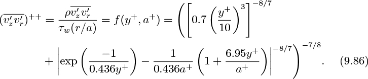
Here, the form and values of the coefficients have been chosen by a variety of methods to give the best fit to available evidence.
The seemingly curious arrangements of the exponents comes directly from an ingenious way of interpolating between two asymptotes or limiting values, documented by Churchill and Usagi10:
10 S.W. Churchill and R. Usagi, “A general expression for the correlation of rates of transfer and other phenomena,” American Institute of chemical Engineers Journal, Vol. 18, p. 1121 (1972).
The functions y0(x) and y∞(x) are arranged so that they dominate, respectively, at the opposite extremes of the range of values of x, so that y(x) is correctly represented at these extremes. The exponent p is chosen to represent the data most accurately between these limits.
Churchill11 points out that the primary purpose of the correlation of Eqn. (9.86) is to provide predictions for ![]() and
and ![]() that are almost exact. Starting from Eqn. (9.85), substituting for
that are almost exact. Starting from Eqn. (9.85), substituting for ![]() from Eqn. (9.86), noting that y = a − r, and rearranging, we have:
from Eqn. (9.86), noting that y = a − r, and rearranging, we have:
11 Private communication, April 2005.

After expressing vz and y in dimensionless form, this differential equation may be integrated successively to give the velocity profile and the mean velocity, and hence—by a development similar to that in Section 9.7—the friction factor.
An additional article by Churchill, Shinoda, and Arai gives an excellent historical review of several correlative strategies for turbulent flow in pipes.12
12 S.W. Churchill, M. Shinoda, and N. Arai, “An appraisal of experimental, predictive, and correlative contributions to fully developed turbulent flow in a round tube,” Thermal Science & Engineering, Vol. 10, No. 2 (2002).
9.12 Computation of Turbulence by the k–[epsilon1] Method
Mixing-length theory as presented in the first part of this chapter provides a good explanation for turbulent velocities in a pipe, but suffers from two insurmountable drawbacks as the basis for turbulent flow in more general situations:
1. It essentially describes a local phenomenon. But turbulence at one location could easily be influenced by convection currents from turbulence upstream, or even downstream in the case of a recirculating flow—as in the eddies for the orifice plate in Fig. 2.19 or the sudden expansion in Fig. 2.21.
2. It cannot predict turbulent flow patterns for any new situation that involves complex geometry.
Hitherto, mixing-length theory gave a turbulent velocity fluctuation, such as ![]() , that was proportional to the mean velocity gradient, such as
, that was proportional to the mean velocity gradient, such as ![]() in Eqn. (9.21). But Prandtl and Kolmorogov reasoned that it would be more logical to relate quantities such as
in Eqn. (9.21). But Prandtl and Kolmorogov reasoned that it would be more logical to relate quantities such as ![]() and the Reynolds stresses to a property of the turbulence itself . Two such properties are:
and the Reynolds stresses to a property of the turbulence itself . Two such properties are:
1. The turbulent kinetic energy per unit mass of the fluctuating components: ![]() , with dimensions L2/T2. In index notation, where summation is implied for repeated subscripts, the kinetic energy can also be written as
, with dimensions L2/T2. In index notation, where summation is implied for repeated subscripts, the kinetic energy can also be written as ![]() .
.
2. The turbulent dissipation rate ε of this kinetic energy, with dimensions L2/T3.
Recall from Example 5.9 the vector form of the three momentum balances for a fluid of constant density but variable viscosity:
For turbulent flow, the Reynolds stresses can be included by enhancing the molecular viscosity μ with the turbulent eddy viscosity ρνT. Bearing in mind that the time-averaged velocity ![]() and pressure
and pressure ![]() are now involved, we have:
are now involved, we have:
in which the continuity equation has been included for completeness.
The k–ε method asserts that the eddy kinematic viscosity at any point should depend only on k and ε at that point. Since νT has dimensions L2/T, it follows that:
in which Cμ is the first of five adjustable coefficients.
We are then faced with the problem of how to compute k and ε as functions of time and position. Starting from the time-averaged equations of motion, and also considering the rate of dissipation of energy by viscous action, a long and involved derivation, with a small amount of empiricism, leads to the transport equation for the kinetic energy. The reader who wishes to learn the details of this and/or related matters, is referred to a number of sources.13, 14, 15, 16, 17 Here, we only really need the final transport equation for the turbulent kinetic energy:
13 B.E. Launder and D.B. Spalding, Lectures in Mathematical Models of Turbulence, Academic Press, London, 1972.
14 H. Tennekes and J.L. Lumley, A First Course in Turbulence, The MIT Press, Cambridge, MA, 1972.
15 P.A. Libby, Introduction to Turbulence, Taylor & Francis, Washington, D.C., 1996.
16 P.A. Durbin and B.A. Petterson Reif, Statistical Theory and Modeling for Turbulent Flows, Wiley & Sons, Ltd., Chichester, 2001.
17 J. Mathieu and J. Scott, An Introduction to Turbulent Flow, Cambridge University Press, Cambridge, 2000.

Largely by analogy—that is, with less rigor—a similar equation governs variations of the dissipation rate:

The five model constants have been chosen so that the k–ε method gives predictions that conform reasonably well with experiments:
The k–ε method is implemented by solving Eqns. (9.90a), (9.90b), (9.92), and (9.93) simultaneously—a daunting task indeed, and one that must be performed by the digital computer. An additional problem occurs in that the equations either start to break down in the viscous layer next to a boundary wall, or would need an impossibly fine mesh in the wall region to achieve accurate results. One approach, implemented by COMSOL, is to assume (quite reasonably) that the velocity component parallel to the wall is a logarithmic function of the distance from the wall, as in the universal velocity profile. If needed, complete details can be found in one of the COMSOL manuals.18
18 For example, COMSOL Documentation in the Help pull-down menu when running COMSOL Multiphysics.
Two examples of software for implementing the method are presented in this book—COMSOL (based on the finite-element method) in the present chapter and Fluent (based on the finite-volume method) in Chapter 13. As with all simulations, the user should at least ponder—do the results appear reasonable or not? Certainly, even though it gives reasonably good results in many circumstances, we should have no illusion that the k–ε method can completely solve all turbulent-flow problems.
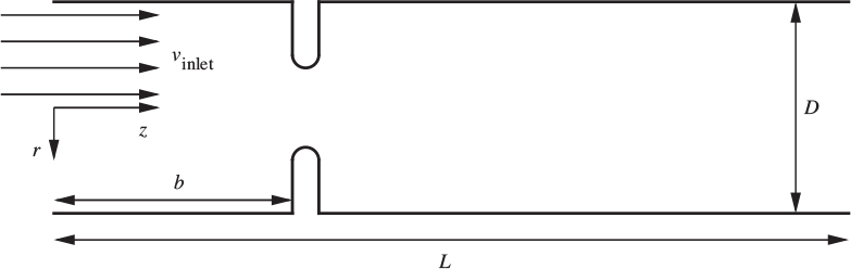
Use COMSOL to investigate the flow pattern in a short segment of pipe that contains an orifice plate, as presented in Fig. 2.19. The fluid is water, with density ρ =62.4lbm/ft3 and kinematic viscosity ν =1.077×10⁻⁵ ft2/s. The dimensions in feet represented in Fig. E9.4.1 are L =0.5, D =0.1, and b =0.1. The dimensions of the intrusion representing the orifice plate are given in Steps 5–7 below. The axial inlet velocity is uniformly vinlet = 1.0 ft/s (with zero radial velocity u0), corresponding to a Reynolds number of 9,285, well in the turbulent-flow region even upstream of the orifice plate. The exit pressure is zero.
Fig. E9.4.1. Geometry of an orifice plate in a pipe.
Make diagrams of the following:
1. The finite-element mesh.
2. Streamlines (time-averaged, as for all subsequent values).
3. Surface plots for velocity magnitudes and turbulent kinematic viscosity, kinetic energy, and logarithm of the dissipation rate.
Solution
See Chapter 14 for more details about COMSOL Multiphysics. All mouse-clicks are left-clicks (the same as Select) unless specifically denoted as right-clicks (R).
Select the Physics
1. Open COMSOL and L-click Model Wizard, 2D Axisymmetric, Fluid Flow (the little rotating triangle is called a “glyph”), Single Phase, Turbulent Flow, Turbulent Flow k–ε, Add. Note that COMSOL uses the symbols u, v, w for the velocity components, k for the turbulent kinetic energy, and ep for the turbulent dissipation rate.
2. L-click Study, Stationary, Done.
Define the Parameters
3. R-click Global Definitions and select Parameters. In the Settings panel to the right of the Model Builder panel enter the parameter rho1 in the Name column and 62.4 [lb/ft3] (as lb/ft^3) in the Expression column. Similarly, enter the kinematic viscosity nu1 as 1.077e-5 [ft2/s] and the inlet velocity, Vinlet, as 1.0 [ft/s]. Note the automatic conversion to SI units.
Establish the Geometry
4. R-click Geometry and select Rectangle. Enter the values for Width and Height as 0.05 [ft] and 0.5 [ft]. Note the default setting is based on the lower left corner being at (0,0). L-click Build Selected.
5. R-click Geometry and select Rectangle. Enter the values for Width and Height as 0.02 [ft] and 0.01 [ft]. Change the coordinate (r, z) of the lower left corner to 0.03 [ft] and 0.1 [ft]. L-click Build Selected.
6. R-click Geometry and L-click Boolean and Partitions, Difference. Select the object to add by L-clicking the large rectangle. Activate the Objects to subtract by L-clicking the On/Off toggle and selecting the small rectangle by L-clicking. L-click Build Selected.
7. R-click Geometry and select Circle. Enter 0.005 [ft] as the Radius and change the r and z values of the center to 0.03 [ft] and 0.105 [ft]. L-click Build Selected.
8. R-click Geometry and L-click Boolean and Partitions, Difference. Select the object from Step 6 by L-clicking it, to add it to the Objects to add. Activate the Objects to subtract by L-clicking the On/Off toggle and selecting the circle by L-clicking. L-click Build Selected.
Define the Fluid Properties
9. R-click the Materials node within Component 1 and select Blank Material. Note that the new material must have the required material parameters that we desire. Enter the parameters rho1 and nu1*rho1 as the values for Density and Dynamic viscosity. Click Turbulent Flow k-ε and then the Equations glyph under Settings, to see the equations being solved.
Define the Boundary Conditions
10. Select the Wall 1 and Axial Symmetry 1 nodes in the Turbulent Flow k-ε tree and inspect the corresponding boundaries in blue. Note the default wall boundary condition is Wall Functions.
11. R-click Turbulent Flow k-ε and select Inlet to define an inlet boundary condition. L-click to select the lowest edge, which is the inlet. Change the value for U0 to Vinlet.
12. R-click Turbulent Flow k-ε and select Outlet to define an outlet boundary condition. L-click to select the top edge, which is the outlet. Note the default is Pressure outlet and the reference pressure is zero.
Create the Mesh and Solve the Problem
13. L-click the Mesh node and note the Element size is Normal. L-click Build All. R-click Mesh, Statistics, and note there are 18,078 elements.
14. R-click Study 1 and select Parametric sweep. In the Settings panel, locate the Study settings. At the bottom of the Parameter definition, L-click the plus icon to add a parameter to the study. You can now use the drop-down box to select nu1 . Enter the values 1.077e-3, 1.077e-4, 1.077e-5, in the parameter list and set the parameter unit to ft^2/s (note: brackets must not be used here—they will lead to an error notice). As a result, COMSOL will start with an artificially high viscosity (100 times its true value) in order to dampen out any instabilities, and then approach the solution by gradually decreasing the viscosity until its true value is reached. The intermediate value 1.077e-4 means that the current solution at that stage (when the viscosity is 10 times its true value) will be saved and will be available for eventual plotting if needed.
15. R-click the Study node and select Compute. You can watch the progress of the solution by clicking on the Progress button under the Graphics window. Observe that there are 51,820 degrees of freedom—that is, the number of unknowns in the simultaneous nonlinear equations being solved (including any Dirichlet boundary conditions). The solution took about five minutes on the author’s Mac Book Pro computer. (For a similar solution using the “Coarse” mesh, there were 9,702 elements and 29,585 degrees of freedom, and the solution took about one minute.)
Explore the Solution, Starting with the Mesh
16. R-click Results and L-click 2D Plot Group. In the Settings window, select the final parameter of interest for the value of nu1 , i.e. 1.077e-5 in the Data section.
17. R-click the new 2D Plot Group 5 and L-click Mesh. Set the Element color to White. The mesh will probably appear without clicking on Plot.
Streamlines
18. R-click Results and L-click 2D Plot Group.
19. R-click the new 2D Plot Group 6 and L-click Streamline. In the Settings window, note the correct velocity components u and w are selected. Change the Positioning to Start point controlled. Again, the plotting will probably be automatic.
Turbulent Kinematic Viscosity, Kinetic Energy, and Dissipation Rate
20. Right-click Results and L-click 2D Plot Group.
21. Right-click the new 2D Plot Group 7 and L-click Surface 7. In the Settings window, change the Expression being plotted by L-clicking the Expression Builder (triangular glyphs) to the far right of Expression (see Fig. E11.3.5) and L-click Component 1, Turbulent Flow k-ε, Turbulence variables, spf.nuT—Turbulent kinematic viscosity. L-click Plot. Alternatively, you could simply have entered the name spf.nuT (where spf denotes single-phase flow).
22. Study the plot and change the Expression to Turbulent Kinetic Energy, either using the Expression Builder or by simply using the name k.
Fig. E9.4.2. (a) Finite-element mesh (extra-coarse, for clarity—normal was used for the actual solution), (b) streamlines (with arrow showing the general direction of flow), and (c) a surface plot showing the magnitudes of the velocity. The abscissas and ordinates give distances in meters.

23. Again study the plot and change the Expression to log(ep), the logarithm to base e of the dissipation rate, which will enable a better overall representation of the areas with the lower values of ep (the high value of which is very largely concentrated at the tip of the orifice plate).
Pressure Cross-Plot
24. Create a data set along the axis of symmetry. R-click Data Sets within the Results tree and select Cut Line 2D. In the Settings window, enter the values (0.0, 0.0) and (0.0, 0.5), each number being followed by [ft], for Points 1 and 2. L-click Plot near the top of the Settings window to display the cut line.
25. R-click Results and L-click 1D Plot Group. In the Settings window, L-click the dropdown dialog and change the data set to Cut Line 2D 1. Make sure that you select the correct parameter value for nu1 , by changing the Parameter selection to Last.
26. R-click the 1D Plot Group 8 and select Line Graph. In the Settings window, change the Expression to Plot to pressure p. In the Coloring and style section, change the Color to Black. L-click Plot.
Fig. E9.4.3. Surface plots of (a) turbulent kinematic viscosity νT , (b) turbulent kinetic energy k, and (c) loge (logarithm to the base e) of the turbulent dissipation rate ep. Arrows show the general direction of flow. The abscissas and ordinates give distances in meters.

Discussion of Results
(a) The “normal” finite-element mesh was used for the calculations, but is too fine to show any detail if reproduced here. Instead, we display an “extra coarse” mesh, containing 3,281 elements. Observe that COMSOL concentrates the elements near the walls, and especially at the orifice plate. It is in these locations that the highest velocity gradients will be encountered.
(b) The streamlines represent the time-averaged motion, and not the paths taken by the water. Observe the contraction through the orifice and the very substantial recirculating eddy in the “backwater” just downstream of the orifice plate.
(c) The surface plot shows the magnitude of the velocity. Since some of the information from the original color is lost in black-and-white, we have added boxes that show general trends of values. Either by observing the original color bar at the right, or clicking on various parts of the diagram, the highest velocity is found to occur on the centerline, a little downstream from the orifice (0.05 m or about 0.16 ft from the inlet), with a value of about 1.48 m/s or 4.85 ft/s, which compares with the inlet velocity of 1.0 ft/s.
Here, we present three more surface plots, perforce reduced from color to black-and-white, but with added labels that show relative magnitudes. In each case, there is a “plume” emanating from the orifice, in which the turbulent effects are greatly enhanced.
(a) In the plume, the turbulent (kinematic) viscosity, νT , continues to increase in intensity all the way to the exit. The maximum value of νT is about 5.9×10⁻³, almost 550 times the molecular kinematic viscosity. The values can be placed in perspective by noting that νT = Cμk2/ε, and comparing νT with k and ε from the turbulent kinetic energy (k) and dissipation (ep) figures.
(b) The turbulent kinetic energy first continues to increase along the plume, but has subsided considerably by the time the flow reaches the exit.
(c) The turbulent dissipation rate is extremely high at the orifice plate, and indeed its value there completely overshadows its value at all other locations. On a linear plot, there is an extremely high spot at the orifice plate, but low everywhere else. A much better ides of the distribution can be obtained by plotting the logarithm (to base e) of ε, log(ep), as shown here. Note that the general distribution is roughly the same as that of the turbulent kinetic energy, but that it decays somewhat faster.
Here, we see a cross-plot of the pressure along the centerline, from inlet to exit. As the velocity increases from 1.0 to about 4.85 ft/s, there is—from Bernoulli’s equation—a sharp but smooth reduction in pressure as the vena contracta is reached at z . = 0.13 ft. Thereafter, as some kinetic energy is converted back to pressure energy, there is some recovery of pressure as the exit is approached, in agreement with the macroscopic analysis on page 87.
Fig. E9.4.4. Variation of pressure from 720 Pa at the inlet to zero at the outlet. The abscissa is the distance from the inlet (m).
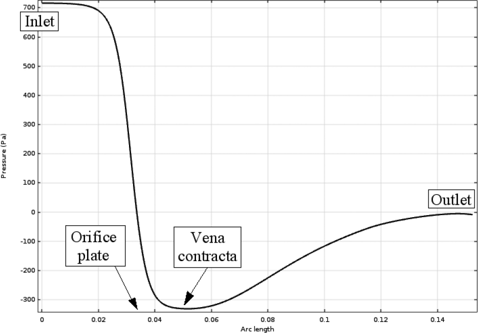
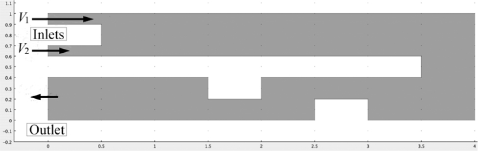
Fig. E9.5.1. Flow of jets into a channel. The axes are in meters.
Problem Statement
Consider the duct in the x/y-plane shown in Fig. E9.5.1, in which the dimensions are in meters, and which extends indefinitely normal to the plane of the diagram. Two reacting gases, each with density ρ = 1.18 kg/m3 and kinematic viscosity ν = 1.83 × 10⁻⁵ m2/s, enter at the top left with velocities V1 = 30 m/s and V2 = 10 m/s, and leave at the bottom left at zero pressure.
(a) Calculate the Reynolds number (based on the channel width of 0.4 m after the gases have mixed) and verify that the flow is likely to be turbulent (Re > 5,000, say).
(b) If the flow is indeed turbulent, use COMSOL to solve the problem using the k–ε method.
(c) Construct the following plots and comment on them:
1. Velocity magnitude.
2. Turbulent kinematic viscosity.
3. Pressure.
4. Logarithm of the turbulent kinetic energy.
5. Logarithm of the turbulent dissipation rate.
6. Arrows that show the velocity vectors.
7. Streamlines.
Solution
Chapter 14 has more details about running COMSOL Multiphysics. All mouse clicks are left-click (the same as Select), unless specifically denoted as R-Click.
check the Reynolds Number
Note that the width of each inlet is 0.1 m and the width after mixing is W = 0.4 m. The mean velocity after mixing is therefore ![]() . Thus, the Reynolds number is
. Thus, the Reynolds number is ![]() , highly turbulent.
, highly turbulent.
Select the Physics
1. Open COMSOL and L-click Model Wizard, 2D, Fluid Flow (the little rotating triangle is called a “glyph”), Single Phase, Turbulent Flow, Turbulent Flow k–ε, Add. L-click Study, Stationary, Done.
Define the Parameters
2. R-click Global Definitions and select Parameters. In the Settings window to the right of the Model Builder enter the parameter rho1 in the Name column and 1.18 [kg/m3] (as kg/m^3) in the Expression column. Similarly, enter the kinematic viscosity nu1 as 1.83e-5 [m2/s] and the two inlet velocities, V 1 and V 2, as 30 [m/s] and 10 [m/s], respectively. For later convenience, define the dynamic viscosity mu1 using the expression nu1 * rho1.
Establish the Geometry
3. Create the geometry using simple rectangles and Boolean operations. Right-click Geometry 1 and select Rectangle to create the rectangle r1. Enter the values for Width and Height as 4 [m] and 1 [m]. Note the default position is based on the lower left corner being located at (0,0). The units may be omitted because the default is [m]. L-click Build Selected.
4. Similarly, create the following four rectangles with width, height, and base combinations: r2, Size (3.5, 0.2), Base (0.0, 0.4); r3, Size (0.5, 0.2), Base (0.0, 0.7); r4, Size (0.5, 0.2), Base (1.5, 0.2); and r5, Size (0.5, 0.2), Base (2.5, 0.0). L-click Build All.
5. Form the final geometry. R-click Geometry and L-click Boolean and Partitions, Difference. Select the largest rectangle, r1, by L-clicking it and note that it appears under Objects to add. Activate the Objects to subtract by L-clicking the On/Off toggle and select the remaining embedded rectangles, r2 through r5, to include them under Objects to subtract. L-click Build Selected. Define the Fluid Properties
6. R-click the Materials node within Component 1 and select Blank Material. Enter rho1 and mu1 as the values for Density and Dynamic viscosity. Define the Boundary Conditions
7. Select the Wall 1 node in the Turbulent Flow k–ε tree and inspect and note that the default wall boundary condition is Wall functions. R-click Turbulent Flow k–ε and select Inlet to define the first inlet boundary condition, Inlet 1. L-click to select the highest left edge (#7), which is Inlet 1. Change the value for U0 to V 1. Similarly, add the second inlet boundary condition, Inlet 2, by selecting the next lower edge (#4) and setting U0 to V 2.
8. Define the zero-pressure outlet condition. R-click Turbulent Flow k–ε and select Outlet to define an outlet boundary condition. L-click to select the lowest left edge (#1), which is the outlet. Note the default is Pressure outlet and the reference pressure is zero. Additionally, ensure the Suppress backflow is deselected and Normal flow is selected. Click Turbulent Flow k–ε and then the Equations glyph under Settings, to see the equations being solved.
Create the Mesh and Solve the Problem
9. L-click the Mesh node and set the Element size to Fine, which is a reasonable starting size for the mesh. L-click Build All and use the graphics function to zoom and inspect the default boundary layer mesh. The image may be moved around by “grabbing” it while holding the Control key down. After a R-click on Mesh 1, note under Statistics that there are 36,886 elements—and 137,685 degrees of freedom (unknowns) to be solved.
10. Following the recommendations in “Wall Functions” on page 744, modify the boundary-layer mesh. Within the Mesh node, under Settings, change the Sequence type to User-controlled mesh, allowing custom setting for the boundary layer mesh. Note that the original mesh setting in the previous step is propagated to the present user settings. Expand the Boundary Layers node by L-clicking on the glyph to its left and L-click Boundary Layer Properties. Change the Number of boundary layers, Boundary layer stretching factor, and Thickness adjustment factor to 8, 1.1, and 1, respectively, as shown in Fig. E9.5.2. This will produce a boundary mesh with reasonable wall lift-off in viscous units. L-click Build Selected.
Fig. E9.5.2. Entries for Boundary Layer Properties.
11. Save the model file periodically.
12. R-click the Study node and select Compute. This will take more time to solve than other examples. Above the Graphics window, L-click the Convergence Plot tab to watch the solution convergence (466 s for the author’s computer), resulting in a surface plot of the velocity magnitude.
13. Inspect the default results for this physics. Particularly note the default Wall Resolution plots and refer to the explanation on page 744. Construct the Necessary Plots
14. Make a surface plot to inspect solution variables. R-click Results and L-click 2D Plot Group. R-click the new 2D Plot Group 4 and L-click Surface. In the Settings window, change the Expression being plotted by L-clicking the Expression Builder (the little triangular glyph) at the right of Expression and Left-click Component 1, Turbulent Flow k–ε, Turbulence variables, spf.nuT - Turbulent kinematic viscosity. L-click Plot.
15. R-click Results and L-click 2D Plot Group. R-click the new 2D Plot Group 5 and L-click Surface. In the Settings window, replace the Expression with the variable p, which is pressure. L-click Plot.
16. Repeat Step 15 using 2D Plot Group 6 and log(k), the logarithm of the turbulent kinetic energy (which gives a better overview than k itself). L-click Plot (not shown here).
17. Repeat Step 15 using 2D Plot Group 7 and log(ep), the logarithm of the turbulent dissipation rate (which gives a better overview than ep itself). L-Plot.
18. Create an arrow plot to visualize flow direction. R-click Results and L-click 2D Plot Group 8. R-click the newly created plot group and L-click Arrow Surface. L-click Plot to update the vector scene. Note that the default arrow resolution is too low to visualize the flow. In the Settings Panel, modify the number of x and y grid points to be 40. L-click Plot to update the scene.
19. Display the streamlines. R-click Results and L-click 2D Plot Group 9. R-click the new 2D Plot Group and L-click Streamline. Several recirculation zones in this example present an issue for defining the streamline starting positions. So, change the Positioning option in the Streamline Positioning section of the Settings panel to Uniform density. Change the Separating distance to 0.01. L-click Plot.
Display of Results and Comments
Fig. E9.5.3. Streamlines showing the time-averaged motion. The faster-moving upper jet entrains the slower-moving lower jet and also creates two clockwise-rotating vortices (C). In the bottom part, there is a slower-moving vortex immediately after each “step”—A (counter-clockwise) and B (clockwise).
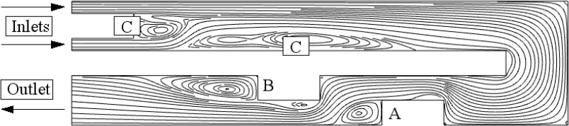
Fig. E9.5.4. Arrow plot. The fast-moving upper jet spreads out and decelerates as its momentum is transferred in the transverse direction by turbulence. The higher velocities are at A (incoming upper jet) and B and C (constricted areas).
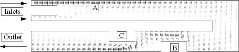
Fig. E9.5.5. Velocity magnitudes. In the original, the color bar at the right ranges from low (blue) to high (red). The very high values occur as the upper jet comes in at A, and also at the two constricted areas at B and C.

Fig. E9.5.6. Turbulent kinematic viscosity νT . The very high values occur well downstream from the inlet and the two lower constrictions. The highest value of the turbulent kinematic viscosity is about 0.170 m2/s, some 9,290 times the molecular kinematic viscosity ν =1.83 × 10⁻⁵ m2/s.

Fig. E9.5.7. Logarithm of the turbulent dissipation rate ε, very low for the slow-moving entrance lower jet A, and very rapidly increasing as the flow impinges against the sharp corners at B and C. If ε (and not its logarithm) were plotted, the two high areas would dominate and everything else would appear quite low and uniformly indistinct in comparison.

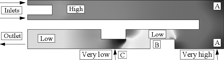
Fig. E9.5.8. Pressure distribution, naturally high at the inlet and low at the exit. The stream stagnates at the two corners marked A, resulting in very high pressures at those locations. Because of the reduced area for flow at B and C, the fluid accelerates and there is a reduction of pressure because of the Bernoulli effect. Near the exit, there is a deceleration and the pressure recovers somewhat.
9.13 Analogies Between Momentum and Heat Transfer
The fact that turbulent eddies can transport heat and mass as well as momentum has already been mentioned in Section 9.3. The question then arises—for example—can an experimental observation on momentum transport be used to make a prediction about heat transfer? The answer, as we shall see, is yes, provided that a realistic model is used.
The Reynolds analogy
Fig. 9.13 shows the simplest model, used in the Reynolds analogy, in which idealized turbulent eddies are constantly moving in both directions between the turbulent “core,” or mainstream, and the walls of the containing duct or pipe. Let m denote the mass flux (mass per unit time per unit area) of such motion in either direction. The rate of transport of z momentum from the mainstream to the wall is ![]() , where
, where ![]() is the mean velocity in the mainstream; in the reverse direction it is
is the mean velocity in the mainstream; in the reverse direction it is ![]() , since the velocity
, since the velocity ![]() at the wall is zero. The difference between these two rates of transport corresponds to a net shear force exerted by the fluid on the wall:
at the wall is zero. The difference between these two rates of transport corresponds to a net shear force exerted by the fluid on the wall:
Net rate of momentum transport:
Fig. 9.13. Momentum and heat transport by turbulent eddies.

By the same token, the rate of heat transport from the mainstream to the wall is ![]() , where
, where ![]() is the mean temperature in the mainstream and cp is the specific heat; in the reverse direction it is
is the mean temperature in the mainstream and cp is the specific heat; in the reverse direction it is ![]() . The difference between these two rates of transport corresponds to a net heat flux from the mainstream to the wall:
. The difference between these two rates of transport corresponds to a net heat flux from the mainstream to the wall:
Net rate of heat transport:
The unknown mass flux m is conveniently eliminated from Eqns. (9.95) and (9.96):
Division by ![]() gives:
gives:
But the first group is just half the Fanning friction factor, fF/2 ; from the definition of the heat-transfer coefficient, h, we can also substitute ![]() , giving: 1 2
, giving: 1 2
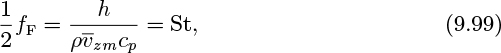
in which St is a dimensionless group known as the Stanton number.
Note that each of the dimensionless groups in Eqn. (9.99) has a ready physical interpretation. The friction factor measures the ratio of the overall momentum transport (to the wall) to inertial effects in the mainstream; and the Stanton number indicates the relative importance of the overall heat transport (to the wall) to convective effects in the mainstream. In effect, the Reynolds analogy simply states that these two ratios are identical, because the same basic model has been assumed for both momentum and heat transfer.
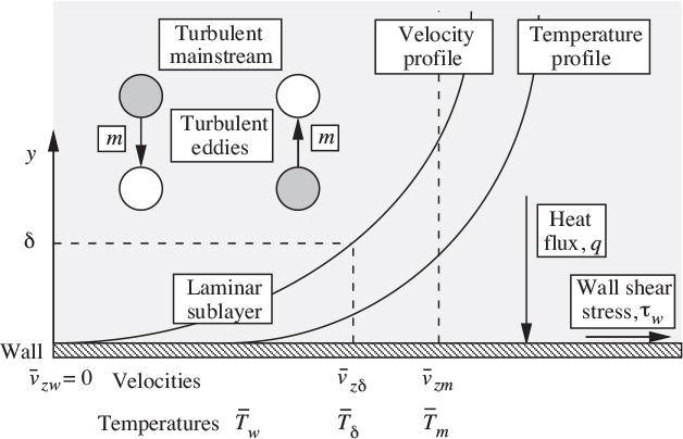
Prandtl-Taylor analogy
An obvious refinement to the Reynolds analogy, which is employed in the Prandtl-Taylor analogy, is to insert between the wall and the eddies a laminar sublayer, of thickness δ, in which turbulent effects are negligible, momentum transport being determined by viscous action and heat transport being controlled by thermal conduction. Referring to the general scheme and notation shown in Fig. 9.14, and assuming linear velocity and temperature variations in the very thin laminar sublayer, the two transport rates are now:
Net rate of momentum transport:
Net rate of heat transport:

Fig. 9.14. Addition of a laminar sublayer to the turbulent mainstream.
Either of these last two pairs of equations can be divided by the other in order to eliminate both δ and m. Either ![]() or
or ![]() can then be eliminated from the remaining two equations, the former being preferred since little is known about it. Several lines of algebra, including the manipulations already seen in the Reynolds analogy, lead to:
can then be eliminated from the remaining two equations, the former being preferred since little is known about it. Several lines of algebra, including the manipulations already seen in the Reynolds analogy, lead to:

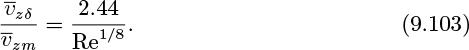
Observe that for Pr = 1, the Prandtl-Taylor analogy simplifies to the Reynolds analogy. Further, from Eqns. (9.61) and (9.62), the required velocity ratio can be shown to be:
Further refinements may be made by inserting a buffer region between the turbulent mainstream and the laminar sublayer. Mass transfer may also be included in the analogies.
Investigate the merits of the Reynolds and Prandtl-Taylor analogies by comparing their predictions for the Nusselt number Nu = hD/k against those obtained from the well-known Dittus-Boelter equation, a correlation that is based on experimentally determined heat-transfer coefficients in smooth pipe:
Solution
1. Reynolds analogy. For simplicity, use the predictions of the Blasius equation for the friction factor, which holds over a fairly wide range of Reynolds numbers:
A combination of Eqns. (9.99) and (E9.6.2) gives:

Multiplication of both sides by ![]() and rearrangement leads to:
and rearrangement leads to:
or:
in which the definitions of the Nusselt and Prandtl numbers have been recognized. Thus, we now have a basis for predicting the heat-transfer coefficient h via the Nusselt number. For a representative Reynolds number of Re = 50,000, Table E9.6 gives in the column “RA” (Reynolds analogy) values of Nu from Eqn. (E9.6.5) for three different Prandtl numbers. Note also the column “DB”, which gives values for Nu from the well-known Dittus-Boelter equation, (E9.6.1), representative of experimental values:
Table E9.6. Nusselt Numbers at Re = 50,000
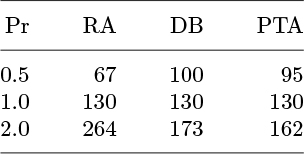
Observe the outstanding agreement at Pr = 1 between the prediction of the Reynolds analogy and the essentially experimental value given by the DittusBoelter equation. Note also the significant differences between the two for Pr = 0.5 and 2. The essence of this discrepancy may be found by reexpressing the Prandtl number as:
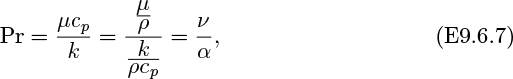
in which ν and α are the kinematic viscosity and thermal diffusivity, respectively. These last two represent the rates at which momentum and heat diffuse through a fluid by molecular action—factors that are completely ignored in the Reynolds analogy.
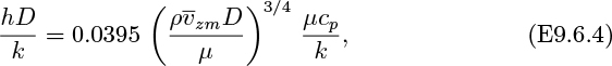
2. Prandtl-Taylor analogy. By similar arguments, if the Blasius equation is again assumed for the friction factor, the Prandtl-Taylor analogy of Eqn. (9.102) yields:
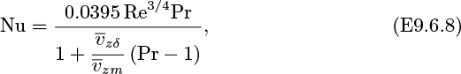
in which the velocity ratio is given in Eqn. (9.103).
The Nusselt numbers predicted from Eqn. (E9.6.8) can also be evaluated, three representative values being given in the last column of Table E9.4. Note that the agreement with the Dittus-Boelter values is now much improved for both Pr = 0.5 and 2, thus illustrating the success of the more realistic Prandtl-Taylor analogy.
9.14 Turbulent Jets
The previous sections in this chapter have discussed turbulence in which the presence of a wall exerted a profound effect on the flow pattern. It is possible to extend the ideas developed so far to the situation of free turbulence, essentially unaffected by such confining boundaries. Two situations are of general interest:
1. The turbulent jet, in which fluid issues from a narrow constriction, to form a turbulent plume of ever-increasing breadth and decreasing velocity.
2. The turbulent wake behind a stationary nonstreamlined object situated in a fluid stream (or an object that is moving in an otherwise stagnant fluid). Again, the wake gradually broadens out downstream.
To a first approximation, both the jet and the wake share five important features in common with the boundary layers discussed in Chapter 8:
1. The flow is primarily in one principal direction, corresponding to the axis of the jet.
2. There is a region of turbulence whose extent gradually increases in the downstream direction.
3. The derivatives of the velocities are considerably larger in the direction trans-verse to the jet or wake than they are in the principal direction of flow.
4. An order-of-magnitude analysis can be used to simplify the equations of motion.
5. In some cases, the solution is facilitated by introducing a stream function.
Under these circumstances, the arguments extended in Section 8.3 for the simplification of the equations of motion still apply, except of course that time-averaged velocities must now be used. There are two further modifications: (a) a turbulent shear stress must be used instead of the viscous stress, and (b) the pressure is essentially constant, apart from a region immediately behind the object in the case of the wake. Only the turbulent jet will be studied here, because it is of greater interest to chemical engineers who are concerned with the rate at which two reactants (represented by the jet and its environment) interact with each other. Two types of jets will be considered:
1. A jet issuing from a long slot—the plane turbulent jet.
2. A jet issuing from a small circular orifice—the axisymmetric turbulent jet.
The plane turbulent jet
First, consider flow in the x/y plane, in which Fig. 9.15 shows fluid issuing to the right from a narrow slotlike opening into a “sea” of fluid in which the pressure is constant. The flow rate is sufficiently high so that the jet is turbulent, and its half-width b increases in the x direction, linearly as it transpires, although this is not assumed a priori. The more usual, but theoretically somewhat more complicated case, of axisymmetric flow will be discussed later. The simplified equations of motion are:
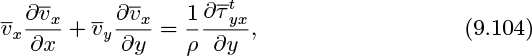
Fig. 9.15. Plane turbulent jet (the broadening effect is exaggerated).

Note the absence of any time derivative—that is, the flow is “steady in the mean.” Also, because the pressure is constant and there is no external force to modify it, the rate of momentum transfer per unit depth in the x direction, ![]() , must be constant:
, must be constant:

Next, consider the turbulent shear stress, for which two treatments are possible, depending on the representation of the eddy kinematic viscosity:
1. From the Prandtl mixing-length theory (this subsection).
2. From a simplified eddy-viscosity theory (the next subsection).
Now proceed with the first of these alternatives. According to the mixing-length theory, which still holds in the absence of a wall, the turbulent shear stress is given by:
in which the underbrace emphasizes the terms that comprise the eddy kinematic viscosity.
As in the case of the boundary-layer problem, we hope that similarity of velocity profiles can be achieved, that this will be expedited by the following assumptions:
1. Paralleling the Blasius solution, a new dimensionless space coordinate ζ can be introduced.
2. The mixing lengthℓ depends only on x, and is directly proportional to b.
3. The half-width of the turbulent zone is proportional to some power p of the x coordinate.
4. The velocity is proportional to a function of ζ and inversely proportional to another power q of x:
The values of p and q can be found by investigating the dependency of each term of Eqns. (9.104) and (9.106) on x. Note that ![]() is of order x−q,
is of order x−q, ![]() is of order x−2q, and the integral of Eqn. (9.106) is of order xp−2q. But since
is of order x−2q, and the integral of Eqn. (9.106) is of order xp−2q. But since ![]() /ρ is constant, it can have no dependency on x, so that:
/ρ is constant, it can have no dependency on x, so that:
By similar arguments, the reader can discover the dependencies on x shown in Table 9.4, in which the continuity equation, (9.108), has been invoked to determine the order of ![]() .
.
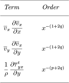
For Eqn. (9.104) to balance, we must have 1 + 2q = p +2q, so that:
Physically, the fact that p = 1 confirms the earlier supposition that the jet spreads linearly with distance ![]() also indicates that the velocities decline proportionally to x−1/2.
also indicates that the velocities decline proportionally to x−1/2.
The solution is expedited by introducing a stream function ψ such that:

Bearing in mind the preceding development, we can now set:
from which the velocities are:

in which the prime denotes differentiation with respect to ζ.
Substitute these expressions for the velocities into the momentum balance, and choose β = (2α2)−1/3 so that α is absorbed into the definition of ζ. After some algebra, Eqn. (9.104) yields an ordinary differential equation in the unknown function f(ζ):

This last equation integrates directly to:

the constant of integration being zero because at the centerline (ζ = 0), considerations of symmetry ![]() give f = f' = 0. A numerical integration of Eqn. (9.115), subject to the initial conditions at ζ = 0 of f = 0 and f' = 1 (an arbitrary choice—the value of γ can then be selected so that the integrated velocity matches any specified flow rate from the jet), yields the plots of f' (needed for
give f = f' = 0. A numerical integration of Eqn. (9.115), subject to the initial conditions at ζ = 0 of f = 0 and f' = 1 (an arbitrary choice—the value of γ can then be selected so that the integrated velocity matches any specified flow rate from the jet), yields the plots of f' (needed for ![]() ) and ζf' − f/2 (needed for
) and ζf' − f/2 (needed for ![]() ) versus ζ, shown in Fig. 9.16.
) versus ζ, shown in Fig. 9.16.
Fig. 9.16. Axial and transverse velocities for plane turbulent jet.

The two time-averaged turbulent velocities ![]() and
and ![]() can then be obtained for any values of γ (determined by the strength of the jet) and the downstream distance x. Finally, note that the numerical results are in complete agreement with the experimental values determined by Förthmann.19 Experimental evidence of Reichardt gives β =7.67, corresponding to α =0.0333.20
can then be obtained for any values of γ (determined by the strength of the jet) and the downstream distance x. Finally, note that the numerical results are in complete agreement with the experimental values determined by Förthmann.19 Experimental evidence of Reichardt gives β =7.67, corresponding to α =0.0333.20
19 As reported on p. 594 of S. Goldstein’s Modern Developments in Fluid Dynamics, Clarendon Press, Oxford, 1957.
20 As reported on p. 500 of Schlichting, op. cit.
As expected, the axial velocity follows a bell-shaped curve, symmetrical about the centerline, with the following characteristics:
1. Since ![]() is plotted, the actual velocities
is plotted, the actual velocities ![]() will decrease as the distance x from the jet increases.
will decrease as the distance x from the jet increases.
2. Because the dimensionless distance ζ = βy/x is plotted, the region in which ![]() is significant will increase as x increases.
is significant will increase as x increases.
That is, the jet simultaneously spreads out and gets slower.
The transverse velocity also shows some interesting features. Consider, for example, positive values of the transverse dimensionless coordinate:
1. For 0 <ζ < 1.25 approximately, ![]() is positive, corresponding to the spreading of the jet.
is positive, corresponding to the spreading of the jet.
2. For the region ζ > 1.25, vy becomes negative and eventually levels out at a significant nonzero negative value, even though the axial velocity is essentially zero. This region corresponds to entrainment of fluid outside the turbulent zone into the jet.
Alternative form for the eddy kinematic viscosity in a plane turbulent jet
An analytical and quicker, but slightly less accurate, solution to the turbulent jet problem is obtained by using a simpler expression for the eddy kinematic viscosity:
in which c is another constant, b is the half-width of the jet, and vxc is the centerline velocity. Observe that the dimensions of νT are still L2/T, and that the model is still physically quite realistic, because the value of νT increases both with:
1. The space available for turbulent fluctuations, as expressed by the half-width b of the jet.
2. The general intensity of velocities, as expressed by the centerline velocity ![]() .
.
The solution again uses the stream function ψ of Eqn. (9.111). Bearing in mind the preceding development, in which b varied linearly with x, we can now set: vxc =

from which the velocities are:

Substitution into the momentum balance and simplification gives:

which integrates once to:
the constant of integration being zero because at the centerline symmetry again gives f = f' = 0. A second integration yields:
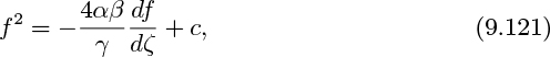
the value of the constant being obtained by noting that at the centerline, f = 0 and f' = 1. Thus, with an appropriate choice for β, we have:

The solution of Eqn. (9.122) and the expression for f' , from which the axial velocity profile can be obtained, are:

This analytical solution agrees quite well with the somewhat more accurate numerical solution displayed in Fig. 9.16, except that it slightly overpredicts the velocities for ζ > 1.5.
The axisymmetric turbulent jet
For a jet issuing from a circular orifice, cylindrical coordinates with axisymmetry are used, as in Fig. 9.17.
Fig. 9.17. Axisymmetric turbulent jet.
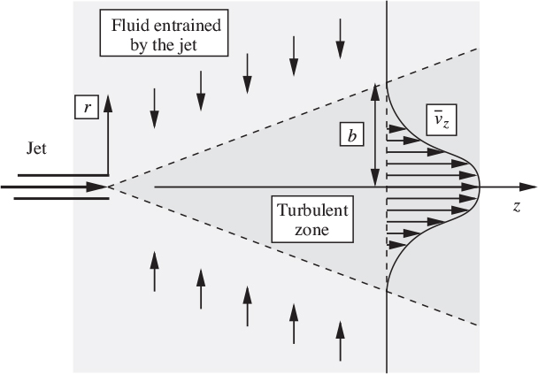
The simplified equations of motion are:

Also, the rate of momentum transfer in the z-direction, ![]() , must be constant:
, must be constant:
The turbulent shear stress and the eddy kinematic viscosity are also given by:

in which c1 is a constant, b is the half-width of the jet, and ![]() is the centerline velocity. Similar to the earlier development of Eqn. (9.108), we can introduce:
is the centerline velocity. Similar to the earlier development of Eqn. (9.108), we can introduce:
From arguments similar to those centered on Eqns. (9.109) and (9.110), and Table 9.4:
The eddy kinematic viscosity νT is therefore constant everywhere, so the equations reduce to:

Although these equations appear formidable, they nevertheless have the following analytical solution, with ![]() again appearing as a bell-shaped curve21:
again appearing as a bell-shaped curve21:
21 See, for example, pp. 161 and 500 of Schlichting, op. cit.
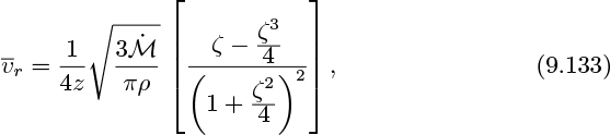
in which:
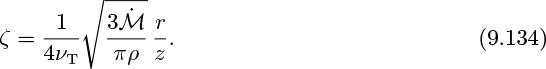
The above theoretical axial velocity profile is well substantiated by the experimental evidence of Reichardt, although the use of mixing-length theory—as opposed to the above assumption of a constant eddy viscosity—gives somewhat better agreement for large values of ζ.22 Reichardt’s experiments also gave ![]() .
.
22 See, for example, p. 501 of Schlichting, op. cit.
Problems for Chapter 9
Unless otherwise stated, all flows are steady state, with constant density and viscosity.
1. Agitation of particles—M (C). A liquid containing a suspension of particles is flowing down a channel inclined at an angle θ to the horizontal. The particles are kept in suspension by the turbulent motion of the liquid, which has a uniform depth λ.
Assuming that the Prandtl mixing length has the form ![]() , where k is a constant, show that the velocity
, where k is a constant, show that the velocity ![]() at a point distant y from the base of the channel may be expressed in the following form, in which c is a constant:
at a point distant y from the base of the channel may be expressed in the following form, in which c is a constant:
Assuming that all the particles settle with the same vertical velocity vg relative to the liquid, and that the mixing length for the particles is the same as for the turbulent motion of the liquid, prove that (except near the lower surface) the number of particles n per unit volume varies with depth according to:
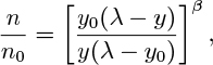
where n0 is the value of n at a distance y0 above the base of the channel, and in which:
If y0 = λ/2, plot n/n0 against y/λ for β = 0.1 and 1. Comment briefly on your results.
2. Logarithmic velocity profile from dimensional analysis—M. For fully developed turbulent flow in a smooth pipe, the following suggestions have been made concerning the distribution of the velocity ![]() :
:
(a) Near the wall, ![]() depends only on ρ, μ, τw, and y, but not on the pipe radius a; that is,
depends only on ρ, μ, τw, and y, but not on the pipe radius a; that is, ![]() . Perform a dimensional analysis along the lines of Section 4.10, and show that
. Perform a dimensional analysis along the lines of Section 4.10, and show that ![]() , where
, where ![]() and
and ![]() .
.
(b) Near the center, the deviation of the velocity from its centerline value ![]() is determined purely by turbulence. That is,
is determined purely by turbulence. That is, ![]() , independent of the viscosity μ. Use dimensional analysis to obtain a functional form for the velocity deviation in this turbulent region.
, independent of the viscosity μ. Use dimensional analysis to obtain a functional form for the velocity deviation in this turbulent region.
(c) If, generally, ![]() , use dimensional analysis to obtain the general functional form for
, use dimensional analysis to obtain the general functional form for ![]() .
.
Hence, if there exists a buffer region in which both (a) and (b) are applicable, demonstrate on dimensional grounds that the velocity profile must be logarithmic in form, both in this buffer region and in the fully turbulent core.
3. Blasius and power-law relationship—E. In Section 9.10 the following statement was made: “There is also another relation between c in the velocity profile and A in the expression for fF.” What is that relation?
4. A novel turbulent velocity profile—M. The suggestion has been made for turbulent flow in a pipe of diameter D =2a that the eddy kinematic viscosity at any location is of the form ![]() , where
, where ![]() is the time-averaged velocity at that location. Based on this model:
is the time-averaged velocity at that location. Based on this model:
(a) What are the dimensions of the constant c?
(b) Give a brief possible explanation for the model.
(c) What is a realistic expression for the turbulent shear stress ![]() at any radius r in terms of the wall shear stress τw?
at any radius r in terms of the wall shear stress τw?
(d) Obtain an expression for the velocity profile ![]() in terms of r, c, a, ρ, τw, and the centerline velocity
in terms of r, c, a, ρ, τw, and the centerline velocity ![]() .
.
(e) Assuming that this velocity profile holds all the way up to the wall, obtain an expression for ![]() that depends only on r, a, and
that depends only on r, a, and ![]() .
.
(f) Evaluate ![]() for r/a = 0, 0.25, 0.5, 0.75, and 1, and comment briefly whether or not this velocity profile is realistic.
for r/a = 0, 0.25, 0.5, 0.75, and 1, and comment briefly whether or not this velocity profile is realistic.
5. Turbulent condensate film—M. Consider the flow of a film of liquid condensate of thickness λ on the outside of a vertical tube, approximated in Fig. P9.5 as a vertical plate.
You are to model the flow in two regimes, without resorting to the universal velocity profile as discussed earlier:
1. A very thin laminar sublayer (LSL) of thickness δ, in which the shear stress is virtually the same as its value τw at the wall.
2. A much thicker turbulent mainstream (TMS), in which the velocity can be assumed to be of the form:
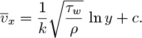
The condensate density is ρ and its viscosity is μ, both assumed constant. Also assume continuity of both the velocity and the velocity gradient at the LSL/TMS junction.
(a) What is the reason for supposing that ![]()
(b) If the liquid flowing down the plate is iso-octane, show that the wall shear stress equals τw . = 81.5 dynes/cm2, and then obtain numerical values for the following:
(i) The thickness δ (cm) of the laminar sublayer.
(ii) The velocity (cm/s) at the LSL/TMS junction.
(iii) The velocity at the free surface of the condensate.
Data (for iso-octane, at 99.3 °C): ρ =0.692 g/cm3, g = 981 cm/s2, μ =0.266 cP = 0.00266 g/cm s, λ =0.12 cm, k =0.40.
Fig. P9.5. Turbulent condensate film with laminar sublayer.

6. Turbulent mixing of reactants—M (C). A constant stream of gas A flows turbulently along a smooth pipe. A relatively small flow rate of a second reacting gas B is to be injected axially by a ring of jets concentric with the axis of the pipe.
At what radius R, expressed as a fraction of the pipe radius a, would you place the ring of jets to give the most rapid initial mixing between A and B? You may assume that:
(a) The most rapid mixing occurs where the eddy diffusivity (taken to be identical with the eddy kinematic viscosity νT) is a maximum.
(b) The velocity profile obeys the one-seventh power law:
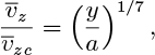
in which ![]() is the centerline velocity.
is the centerline velocity.
7. Pneumatic particle transport—M. A gas of density ρg and viscosity μg flows turbulently with mean velocity ![]() in a horizontal tube of diameter D that is partly filled with solid spherical particles of diameter d and density ρp. At sufficiently high gas velocities, the particles will be agitated by the turbulence and conveyed along the tube by the gas—a phenomenon known as pneumatic transport. We wish to investigate the principal dimensionless group that could be used for correlating experimental data on variables such as flow regimes and the fraction νT of the total volume occupied by the particles.
in a horizontal tube of diameter D that is partly filled with solid spherical particles of diameter d and density ρp. At sufficiently high gas velocities, the particles will be agitated by the turbulence and conveyed along the tube by the gas—a phenomenon known as pneumatic transport. We wish to investigate the principal dimensionless group that could be used for correlating experimental data on variables such as flow regimes and the fraction νT of the total volume occupied by the particles.
Fig. P9.7. Particle at wall in turbulent flow.
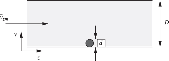
As shown in Fig. P9.7, conduct a preliminary investigation into the gas velocity that is needed to pick up a single particle from its initial position on the wall. Assume the following:
(a) Analogous to the drag on spherical objects in fluid streams, we can define a dimensionless drag coefficient:
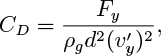
which can reasonably be expected to be constant at sufficiently high Reynolds numbers. Here, Fy is the force exerted in the y direction on the particle due to a sudden transverse velocity fluctuation ![]() .
.
(b) The fluctuation ![]() is proportional to the magnitude of a similar fluctuation
is proportional to the magnitude of a similar fluctuation ![]() in the axial velocity, which is given by a standard expression from mixing-length theory.
in the axial velocity, which is given by a standard expression from mixing-length theory.
(c) The mixing length ℓ' is proportional to the pipe diameter.
Demonstrate from the above that the value of the following dimensionless group is likely to determine whether or not the particle will be picked up from the wall:

8. Velocity at the outer edge of the laminar sublayer—M. Starting from Eqns. (9.61) (the one-seventh power law) and (9.62) (for the thickness of the laminar sublayer), prove Eqn. (9.103), which gives the velocity at the outer edge of the laminar sublayer:
Evaluate this velocity ratio for Re = 104, 105, and 106, and comment on the results.
9. Various quantities in turbulent flow—M. Quoting any formula(s) for the universal velocity profile, prove the following relationship between the dimensionless mean velocity and the dimensionless pipe radius for flow in a smooth pipe:
Comment briefly on any assumptions that have been made in the derivation of this equation.
Water (ρ = 1, 000 kg/m3, μ = 0.001 kg/m s) flows through a hydraulically smooth 5.0-cm (0.05 m) diameter pipe under a pressure gradient of −dp/dz = 14,000 N/m3. Find the wall shear stress (N/m2), the mean velocity (m/s), the Reynolds number, the thickness of the laminar sublayer (m), and the velocity (m/s) at the junction between the laminar sublayer and the buffer region.
Estimate the heat-transfer coefficient (W/m2 °C) between the water and the pipe wall if water has a specific heat of cp =4,184 J/kg °C.
10. An alternative to the Prandtl hypothesis—M. Sleicher proposed that in a region close to the wall, the eddy kinematic viscosity obeys23:
23 C.A. Sleicher, Jr., “Experimental velocity and temperature profiles for air in turbulent pipe flow,” Transactions of the American Society of Mechanical Engineers, Vol. 80, pp. 693–704 (1958).
vT = v(cy+)2.
By considering both turbulent and viscous contributions to the shear stress, which still essentially equals its wall value, prove that the corresponding velocity profile is:
If c = 0.088, show that the above velocity profile merges smoothly—both in magnitude and slope—with ![]() , and discover the value of y+ at which the transition occurs.
, and discover the value of y+ at which the transition occurs.
11. Turbulent mass transfer—D. Considering gas flow of molecular weight Mw in a pipe as represented by a central turbulent core with a laminar sublayer next to the wall, derive the following analogy between mass and momentum transfer when the partial pressure of A is pAm in the mainstream and zero at the wall:
Here, NA is the molal flux, P is the total pressure, and Sc = ν/D is the Schmidt number, where D is the diffusion coefficient across the laminar sublayer.
The catalytic isomerization of butene–1 to butene–2,
CH3CH2CH=CH2 → CH3 CH=CHCH3
is carried out continuously and isothermally at 800 °F and 1 atm in a lime-coated porcelain tube of 2-in. I.D., and with the tube wall serving as the catalyst. Assuming that the rate of reaction is essentially the rate of which butene–1 diffuses to the wall, estimate the length of tube required to give 80% conversion of a pure butene–1 feed. Assume that the laminar sublayer is thin and contributes little to the overall flow, and that the concentration and velocity profiles are flat over most of the turbulent region.
Data: at 800°F, D = 0.59 ft2/hr, μ = 0.044 lbm/ft hr, cf = 0.0086, and uL/um = 0.72.
12. Thickness of the laminar sublayer—M. In Section 9.8, the thickness of the laminar sublayer was shown to be δ/D =58.3/Re7/8 for a logarithmic velocity profile in the mainstream.
Conduct a similar derivation to verify the corresponding result for a velocity profile in the turbulent region given by the one-seventh power law, ![]() . Evaluate this thickness ratio for Re = 104, 105, and 106. Comment on your results.
. Evaluate this thickness ratio for Re = 104, 105, and 106. Comment on your results.
13. Turbulent heat transfer—M (C). In a gas-cooled nuclear reactor, the fissile material is made into straight tubular fuel elements of length L and internal diameter D. Coolant passes through the tubes, which are embedded in a block of moderating material of thickness L, shown in Fig. P9.13. At a distance x from the inlet, the rate of heat production per unit length is q sin(πx/L).
Fig. P9.13. Representative coolant tube in a nuclear reactor.

By using the Reynolds analogy, prove that the position xm at which the temperature at the inner surface of the fuel element is a maximum is given by:
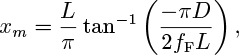
in which fF is the Fanning friction factor.
Assume that an energy balance leads to the following equation for the variation of coolant temperature T with distance x:
where m is the mass flow rate of coolant and cp is its specific heat, h is the heat-transfer coefficient, and Tw is the local wall temperature.
14. Turbulent velocity profile—M (C). A fluid in turbulent flow passes through a smooth circular pipe, and the velocity distribution is given by the equation:

If this equation holds across the whole pipe, calculate the ratio of the maximum velocity to the mean velocity at Re = 105. At what position should a Pitot tube be placed to measure the mean velocity at this Reynolds number?
15. Reynolds analogy for minimum pumping power—M (C). A gas of molecular weight Mw is pumped through a cylindrical coolant duct in order to remove heat from part of a nuclear reactor. The temperature rise ΔT , the logarithmic-mean temperature difference ΔTlog mean, the transfer area A, and heat load q are specified, so in the heat-balance equation:
(4)
the only variables are the mass flow rate m and the specific heat cp of the gas. Thus, mcp is a constant, c1 for example.
Use the Reynolds analogy to prove that the pumping power P = QΔp (where Q is the volumetric flow rate and Δp is the pressure drop in the duct) is lowest if a gas is selected with the largest possible value of ![]() . Assume ρ = Mwp/RT for the gas, with p, R, and T effectively constant, so that ρ = c2Mw, where c2 is another constant.
. Assume ρ = Mwp/RT for the gas, with p, R, and T effectively constant, so that ρ = c2Mw, where c2 is another constant.
16. Turbulent mass flux—E. Consider flow in a pipe of diameter D and length L with a mean axial velocity ![]() . Note that the Reynolds analogy gives the turbulent mass flux per unit area of the wall as
. Note that the Reynolds analogy gives the turbulent mass flux per unit area of the wall as ![]() . Let mt be the total such mass flux based on the total wall area of the pipe. Also define mc as the convective mass flow rate along the pipe. For flow in a smooth pipe of diameter D =0.05 m at a Reynolds number Re = 104, how long would the pipe have to be so that mt = mc?
. Let mt be the total such mass flux based on the total wall area of the pipe. Also define mc as the convective mass flow rate along the pipe. For flow in a smooth pipe of diameter D =0.05 m at a Reynolds number Re = 104, how long would the pipe have to be so that mt = mc?
17. Theory for a plane turbulent jet—D. Prove Eqn. (9.114) from the development that precedes it.
18. Calculation of velocities for a plane turbulent jet—D. (a) Verify that by defining new variables f0 = f and f1 = df/dζ, Eqn. (9.115) can be expressed as two first-order ordinary differential equations:

subject to the boundary conditions:
(b) As discussed in Appendix A, use a spreadsheet to implement Euler’s method (or similar) to solve Eqn. (P9.18.1) subject to the boundary conditions (P9.18.2), from ζ = 0 to a value where the velocities are negligible. (Any other standard software for solving differential equations may be used instead.) Try different step-sizes Δζ to make sure that you have used one that is sufficiently small for accurate results. Plot f' and ζf' − f/2 against both negative and positive values of ζ, one-half of which can be obtained from symmetry.
Hint: if your computed values appear improbable, did you make the right choice when faced with an alternative?
19. Streamlines and velocities for a plane turbulent jet—M. Sketch the streamlines for the turbulent jet, for which the velocities are shown in Fig. 9.16. Include both the jet and the region outside it. Also show the axial velocity profiles at three stages in the development of the jet.
20. Analytical solution for the plane turbulent jet—M. Verify Eqn. (9.123) from the development that precedes it, and compare the numerical values for f' with those deduced from Fig. 9.16.
21. Entrainment by a plane turbulent jet—M. For the plane turbulent jet discussed in Section 9.14, what is the dependency of the total mass flow rate per unit depth in the jet on the axial distance x? Comment critically on your answer.
Assume the “simplified” analytical solution given by Eqn. (9.123).
22. Axisymmetric turbulent jet—D. For the axisymmetric turbulent jet, verify that:
(a) The powers of z appearing in Eqn. (9.128) for ζ and ![]() are p = q =1.
are p = q =1.
(b) The velocities given in Eqns. (9.132) and (9.133) satisfy the appropriate differential momentum and mass balances and that the total rate of momentum transfer is ![]() .
.
23. Entrainment by an axisymmetric turbulent jet—M. For the axisymmetric turbulent jet discussed in Section 9.14, what is the dependency of the total mass flow rate in the jet on the axial distance z? Comment critically on your answer.
24. Streamlines and velocities in an axisymmetric turbulent jet—M. (a) Verify that the velocities in Eqns. (9.132) and (9.133) are consistent with the stream function:

(b) Sketch several streamlines, both within the jet and outside it. Also show the axial velocity profiles at three stages in the development of the jet.
(c) Plot dimensionless axial and radial velocity profiles in the manner of Fig. 9.16.
25. The Prandtl number and the Reynolds analogy—E. Table E9.6 showed that the Reynolds analogy underestimated/overestimated the heat-transfer coefficient for Prandtl numbers lower/higher than one. With reference to the definition of the Prandtl number as the ratio of the kinematic viscosity to the thermal diffusivity, explain on physical grounds why this is so.
26. Order of terms for turbulent jet—E. Verify the orders of the three terms appearing in Table 9.4 relating to a plane turbulent jet.
27. True/false. check true or false, as appropriate:
(a) Turbulent fluctuations typically occur in a matter of microseconds.
T ![]() F
F ![]()
(b) The time-averaged continuity equation contains the time-averaged velocities instead of the instantaneous velocities.
T ![]() F
F ![]()
(c) Extra terms, known as the Reynolds stresses, occur when the momentum balances are time-averaged.
T ![]() F
F ![]()
(d) The Reynolds stresses can be explained by considering the transport of momentum by turbulent eddies.
T ![]() F
F ![]()
(e) Mixing-length theory attempts to unify the turbulent transport of momentum, heat, and mass.
T ![]() F
F ![]()
(f) The Prandtl hypothesis assumes that the mixing lengthℓ does not depend on the distance from the wall.
T ![]() F
F ![]()
(g) The Prandtl hypothesis, in conjunction with the assumption of an approximately constant shear stress, leads to a logarithmic-type velocity profile.
T ![]() F
F ![]()
(h) The laminar sublayer is a thin region next to the wall, in which turbulent fluctuations are essentially negligible.
T ![]() F
F ![]()
(i) A friction factor is the ratio of the wall shear-stress effects to inertial effects.
T ![]() F
F ![]()
(j) In the universal velocity profile, the junction between the laminar sublayer and the turbulent core occurs at approximately y+ = 25.
T ![]() F
F ![]()
(k) The thickness of the laminar sublayer increases as the Reynolds number increases.
T ![]() F
F ![]()
(l) The Colebrook and White equation gives the friction factor for both laminar and turbulent flow in a pipe.
T ![]() F
F ![]()
(m) The Blasius law, fF=0.079Re−1/4, is consistent with the one-seventh power law turbulent velocity profile.
T ![]() F
F ![]()
(n) The Prandtl hypothesis,ℓ = ky, somewhat underestimates the mixing length for general values of y.
T ![]() F
F ![]()
(o) The Prandtl number is the ratio of the kinematic viscosity to the thermal diffusivity.
T ![]() F
F ![]()
(p) If the random fluctuations ![]() and
and ![]() are correlated in some way, then
are correlated in some way, then ![]() will not be zero.
will not be zero.
T ![]() F
F ![]()
(q) In the simple model we discussed for turbulence, the same eddies can transport mass, momentum, and thermal energy.
T ![]() F
F ![]()
(r) A hydraulically smooth pipe is one in which the “hills” on the wall do not extend beyond the laminar sublayer.
T ![]() F
F ![]()
(s) When the general momentum balances are time-averaged, the only significant changes are that time-averaged values (such as ![]() ) have replaced the instantaneous values (such as p).
) have replaced the instantaneous values (such as p).
T ![]() F
F ![]()
(t) For flow in a smooth pipe of diameter D = 12 in with Re = 105, the thickness of the laminar sublayer is 0.138 ± 0.02 in.
T ![]() F
F ![]()
(u) For a turbulent eddy, a high Prandtl number means that its momentum content is likely to be dissipated more quickly than its thermal energy content before it reaches its destination.
T ![]() F
F ![]()