
Chapter 10. Bubble Motion, Two-Phase Flow, And Fluidization
10.1 Introduction
THE simultaneous motion of two or more immiscible fluids is of considerable importance in chemical engineering, and there is an abundance of examples, such as:
1. Mixing of coal particles with water and pumping the resulting slurry through a pipeline.
2. Simultaneous production of oil and natural gas upward through a vertical well.
3. Vaporization of water or other liquids inside the heated tubes of a vertical-tube evaporator.
4. Contacting a reacting fluid with catalyst particles in a fluidized bed.
5. Absorption of a component from a gas stream that is rising through a packed bed in a tower, down through which an absorbing liquid is flowing.
6. Aerated bioreactors, with air bubbles affording a large surface area for reaction.
The complete study of any one of these topics requires much more space than is available here. Indeed, we shall see later that an entire book has been written on one-dimensional two-phase flow, and that another one has been devoted exclusively just to the annular regime in two-phase flow. Nevertheless, the reader will be introduced in this chapter to the important concepts and should gain a substantial insight into the key issues.
10.2 Rise of Bubbles in Unconfined Liquids
In order to predict the performance of two-phase flow in vertical tubes (Section 10.4) and fluidized beds (Sections 10.7 and 10.8), it is first necessary to study the rate of rise of single bubbles.
Small bubbles
The results of Peebles and Garber1 are summarized in Table 10.1 for bubbles with volumes in the range equivalent to spheres with radii between 0.024 and 0.3 in. There are four distinct rise modes, generally corresponding to increasing bubble size (Reb is the Reynolds number of the bubble, based on its rise velocity ub, and Rb is the radius of a sphere having the same volume as the bubble, and is half the equivalent diameter De introduced later):
1 F.N. Peebles and H.J. Garber, “Studies on the motion of gas bubbles in liquids,” chemical Engineering Progress, Vol. 49, No. 2, pp. 88–97 (1953).
1. For Reb < 2, the bubbles behave as buoyant solid spheres, rising vertically, with their motion determined by Stokes’ law.
2. For larger values of Reb (up to a limit determined by properties of the liquid) the bubbles also rise vertically as spheres, but with a drag coefficient slightly less than that of a solid sphere of the same volume.
3. For a range of Reb determined by the liquid properties, the bubbles are flattened and rise in a zigzag pattern, with significantly increased drag coefficients.
4. The largest bubbles rise almost vertically with significantly increasing drag coefficients, and assume irregular mushroom-cap shapes. For this region, the constant 1.53 recommended by Harmathy has been used instead of the value of 1.18 from Peebles and Garber, because it correlates better with experiment.2
2 T.Z. Harmathy, “Velocity of large drops and bubbles in media of infinite or restricted extent,” American Institute of chemical Engineers Journal, Vol. 6, No. 2, pp. 281–288 (1960).
Table 10.1. Terminal Velocities for Bubbles. Values for Regions 1–4 are from Peebles and Garber.
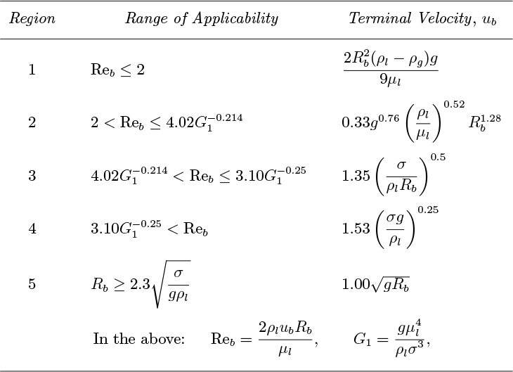
Peebles and Garber also reported the results of Davies and Taylor for larger bubbles (see below), but did not include them in their table. For completeness, however, these have been included under Region 5 in Table 10.1. The limit of bubble radius Rb beyond which Region 5 applies has been obtained by equating the velocities given by Region 4 and Eqn. (10.8) for spherical-cap bubbles.
Large “spherical-cap” bubbles
For otherwise stationary liquids that are not very viscous, the shape of a “large” bubble (whose volume equals that of a sphere whose diameter is several mm) is roughly lenticular or that of a spherical cap, as shown in the upper part of Fig. 10.1. A somewhat similar shape occurs for a large gas bubble rising in a fluidized-bed reactor, although in this case the bubble is more nearly a complete sphere.
Fig. 10.1. Flow around a spherical cap bubble.
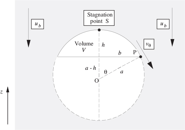
The rise velocity ub of such bubbles is analyzed by first superimposing a downward velocity ub on the whole system, so that we have a downward streaming of the liquid—in potential flow—past a stationary spherical-cap bubble. Because the bubble is large, surface-tension effects are negligible.
Noting that the pressure is constant because of the gas in the bubble, application of Bernoulli’s equation between S and P gives the tangential velocity vθ at point P as:
But, from Eqn. (7.73), for potential flow around a sphere, with U = −ub:

which gives, at the bubble surface r = a:
If the two effects give the same result, (10.1) and (10.3) may be equated, giving:
which can be satisfied for small values of θ (that is, near the bubble “nose” S, where 1 + cos θ . = 2), giving a bubble rise velocity of:
The rise velocity ub can also be obtained in terms of the bubble volume V . Integration over the height of the spherical cap can be shown to give its volume as:
yielding, in combination with Eqn. (10.5):
The experiments of Davies and Taylor gave a similar result:3,4
3 R.M. Davies and G.I. Taylor, “The mechanics of large bubbles rising through extended liquids and through liquids in tubes,” Proceedings of the Royal Society, Vol. 200A, pp. 375–390 (1950).
4 The author attended a G.I. Taylor seminar during the sesquicentennial celebrations of the University of Michigan in 1967. Taylor related the following technique for locating the position of a sailboat lost in a deep fog near a coastline (whose general direction was known). Sail due west (for example) and record the distance traveled until the coast is reached. Return to the original position by sailing due east for the same distance. Then sail north for a known number of miles. Repeat the entire process a few times. On a suitable scale, the result can be transcribed to resemble a comb with a few teeth of unequal length, which can then be adjusted until it fits a map of the coastline, thereby determining the ship’s bearings!
in which the equivalent diameter De of the bubble is defined as the diameter of a sphere that has the same volume as the bubble:
We now need to reexpress ![]() in terms of
in terms of ![]() , so that the Davies and Taylor result of Eqn. (10.8) can be compared directly with the theoretical prediction of Eqn. (10.5). From Eqns. (10.6) and (10.9) and the geometry of Fig. 10.1, a few lines of algebra give two relations for the bubble volume:
, so that the Davies and Taylor result of Eqn. (10.8) can be compared directly with the theoretical prediction of Eqn. (10.5). From Eqns. (10.6) and (10.9) and the geometry of Fig. 10.1, a few lines of algebra give two relations for the bubble volume:
from which the values given in Table 10.2 can be determined.
Table 10.2. Numerical Values for Spherical-Cap Bubbles
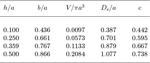
If the Davies and Taylor experimental correlation of Eqn. (10.8) is translated into the form:
then Table 10.2 gives the appropriate values for the coefficient c. The bubble angle that corresponds to the approximate theoretical value c = 2/3 is θ = cos−1(1 − 0.359) = 50.1°. A more accurate treatment would require that the shape of the bubble be adjusted, and the flow pattern recomputed, so that the Bernoulli condition, Eqn. (10.1), is satisfied everywhere—not just in the vicinity of the nose.
Plot the rise velocity ub, cm/s, for single bubbles of air in water against the equivalent bubble diameter De, from De = 0.01 to 10 cm.
Solution
From Chapter 1, the physical properties of water at 20 °C are: ρ = 0.998 g/cm3, σ =72.75 dynes/cm (= g/s2), μ =1.21 cP or 0.0121 g/cm s, and g = 981 cm/s2. A spreadsheet is then used to implement the correlations for the five regions of Table 10.1. The results for ub vs. De are shown in Fig. E10.1.
Fig. E10.1. Bubble rise velocity as a function of equivalent diameter.
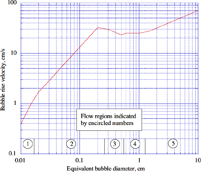
After the peak in ub at the higher end of Region 2, the moderate decline in Region 3 is observed experimentally. The slight jump in passing from Region 3 to Region 4 is a consequence of the correlations used. The Reynolds number range was 0.5–70,420.
10.3 Pressure Drop and Void Fraction in Horizontal Pipes
In this chapter, the discussion of two-phase flow in pipes will center largely on vertical flow because of its importance in gas and oil wells, evaporators, bioreactors, and boilers. However, the topic is introduced by considering two-phase flow in horizontal pipes. Although there are several different regimes in horizontal flow in which the gas and liquid interact with each other in different ways (somewhat similar to those in Fig. 10.3 for vertical flow), a simpler approach is taken in the following model. See Table 10.3 for the notation for this and the next section.
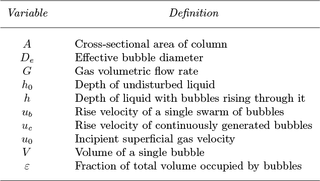
Table 10.3. Variables for Two-Phase Gas/Liquid Flow

The void fraction ε is the fraction of the total volume in the pipe that is occupied by the gas phase, and is related to the individual volumetric flow rates G and L and the mean velocities vg and vl by:
The quality x of the flowing stream (a term used when analyzing the performance of boilers) is the fraction of the total mass flow rate that is in the gas phase:

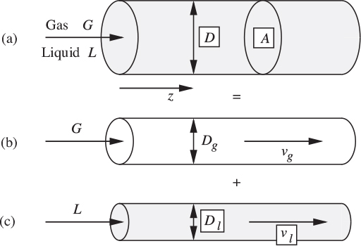
As a first approximation, the frictional pressure drop for two-phase flow in the horizontal tube of diameter D in Fig. 10.2(a) may be deduced by supposing that the gas and liquid flow individually in cylinders of diameters Dg and Dl, respectively, as in (b) and (c). The void fraction is then the ratio of two areas:

Fig. 10.2. Separated horizontal flow model. Simultaneous gas/liquid flow in (a) is considered as the combination of gas and liquid flows, as in (b) and (c).
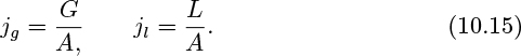
As another preliminary, observe the definitions of two important types of velocities:
1. The superficial velocities are those that would occur if each phase flowed by itself in a pipe of cross-sectional area A, the other phase being absent. Thus, if the volumetric gas and liquid flow rates are G and L, respectively:
2. The mean velocities are the superficial velocities divided by the gas and liquid fractions:
First consider the pressure gradient in the gas, for the following two cases:
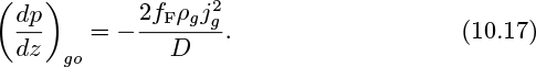
1. Gas only flowing by itself and occupying the entire cross section of the pipe:
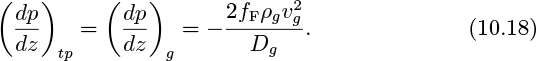
2. Gas flowing by itself in the hypothetical cylinder of diameter Dg. Note that this must also equal the pressure gradient for the combined two-phase flow:
The ratio of these last two equations yields:
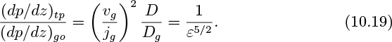
in which Eqns. (10.14) and (10.16) have been used to eliminate the ratios vg/jg and D/Dg in terms of the void fraction.
Equation (10.19) can be rewritten in the form:

Similarly, by considering the pressure drop in the liquid phase:

The use of ϕ2 instead of ϕ perpetuates the notation used by early researchers in the field and has no particular significance.
Elimination of the void fraction from the second relations in Eqns. (10.20) and (10.21) gives: 1 (ϕ2g)2/5
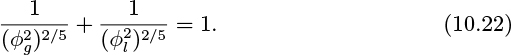
Note that these results are based on a simplified model, and that the same value of the friction factor is also assumed for both phases. Nevertheless, the early studies of Lockhart and Martinelli correlate remarkably well with modest modifications to Eqn. (10.22).5 These researchers investigated a wide variety of liquids flowing with air at roughly atmospheric pressure in small-diameter (up to 1.0–in. I.D.) tubes, and their results are summarized in Table 10.4. They recognized four regimes, comprising all possible combinations of viscous (Re < 1,000) or turbulent (Re > 2,000) flow for each phase, calculated as though it flowed by itself and occupied the whole cross section.
5 See R.W. Lockhart and R.C. Martinelli, “Proposed correlation of data for isothermal two-phase, two-component flow in pipes,” chemical Engineering Progress, Vol. 45, No. 1, pp. 39–48 (1949).
Table 10.4. Values from Lockhart and Martinelli
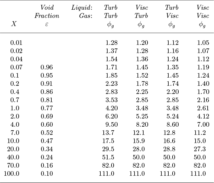
The square of the parameter X is defined as the ratio of the liquid-only and gas-only pressure gradients:

Large or small values of X correspond to a flow regime that is primarily liquid or primarily gas, respectively.
Equation (10.22) is a special case of the more general form:

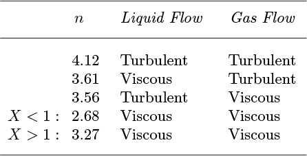
in which the value of n depends on the flow regime as indicated in Table 10.5.
Table 10.5. Exponents for Two-Phase Correlation
The tabulated values of ε are empirically correlated (with an error no larger than 0.02) by:

From Eqns. (10.23) and (10.24):
and it is easy to show from a spreadsheet that the values of Table 10.4 are well represented by Eqn. (10.26) with the exponents given in Table 10.5.
Refinements of the above procedure are available from Baroczy, who investigated a wide variety of fluids, including steam and water up to pressures of 1,400 psia.6 Chisholm has also adapted Baroczy’s work to the prediction of pressure drops in evaporating flows.7
6 C.J. Baroczy, “A systematic correlation for two-phase pressure drop,” chemical Engineering Progress Symposium Series Vol. 62, No. 64, pp. 232–249 (1966).
7 D. Chisholm, “Pressure gradients due to friction during the flow of evaporating two-phase mixtures in smooth tubes and channels, International Journal of Heat and Mass Transfer, Vol. 16, pp. 347–358 (1973).
Gas and oil are flowing at volumetric flow rates G = 10.0, L = 0.5 ft3/s in a horizontal pipeline of internal diameter D = 0.5 ft. Estimate the fraction of gas, the pressure gradient, and the mean velocities of each phase. The physical properties are ρg = 0.15, ρl = 50.0 lbm/ft3, μg = 0.025, μl = 20.0 lbm/ft hr; the Fanning friction factor is fF = 0.0045.
Solution
The following quantities are first calculated:
Cross-sectional area of pipe
Superficial velocities
Reynolds numbers
Thus, the flow is turbulent for the liquid and turbulent for the gas, with n =4.12 from Table 10.5.
The quantity X2, being the ratio of the liquid-only and gas-only pressure gradients is next calculated from Eqns. (10.23), (10.17), and a similar one for the liquid pressure gradient. The friction factor and the diameters are the same in each case and cancel, giving:

From Eqn. (10.26) (or Table 10.4), the value of ϕg is:
From Eqn. (10.25) (or Table 10.4) the fraction of gas is:

The relevant pressure drops are obtained from Eqns. (10.17) and (10.20):
Gas only

Two-phase flow

Finally, the individual mean velocities are obtained:
Gas
Liquid
10.4 Two-Phase Flow in Vertical Pipes
Two-phase gas/liquid flow in vertical pipes will be treated in more detail because of its importance in evaporators and in the simultaneous transport of oil and gas in wells. Several flow regimes can occur, depending on many factors, including the individual magnitudes of the liquid and gas flow rates, and physical properties such as density, surface tension, and viscosity.
There are four principal flow regimes, shown in Fig. 10.3, which occur successively at ever-increasing gas flow rates:
(a) Bubble flow, in which the gas is dispersed as small bubbles throughout the liquid, which is the continuous phase.
(b) Slug flow, in which the individual small bubbles have started to coalesce together in the form of gas slugs. The liquid phase is still continuous. For high gas flows, the liquid “pistons” between the slugs start to narrow down and form irregularly shaped “bridges,” a situation that is known as churn flow.
(c) Annular flow, in which the fast-moving gas stream is now a continuous phase that encompasses the central portion of the pipe, with the liquid forming a relatively thin film on the pipe wall. Partial entrainment of the liquid into the gas stream may occur.
(d) Mist flow, in which the velocity of the continuous gas phase is so high that it reaches as far as the pipe wall and entrains all of the liquid in the form of droplets.
Fig. 10.3. Two-phase flow regimes in a vertical pipe at increasing gas flow rates: (a) bubble, (b) slug, (c) annular, and (d) mist flow. In each case, the gas is shown in white, and the liquid is shaded or black.

Determination of flow regime
A typical situation occurs when the gas and liquid volumetric flow rates G and L are specified, and the pressure gradient dp/dz and void fraction ε are to be calculated. Correlations for these last two variables are more likely to be successful if they can recognize the particular flow regime and develop relationships specifically for it. The following approximate demarcations are recognized:
1. Bubble/slug flow transition. Small bubbles introduced at the base of a column of liquid will usually eventually coalesce into slugs. The transition depends very much on the size of the bubbles, how they were introduced, the distance from the inlet, and on surface-tension effects, so there is no simple criterion for the transition. Also, for practical purposes of determining pressure gradients and void fraction, an exact knowledge of the transition point is unlikely to be needed. Experiments of Nicklin indicate that the correlation for the void fraction based on slug flow (see below) extends accurately into the bubble region for void fractions as low as a few percent.8 It appears that if a void fraction of ε = 0.1 is somewhat arbitrarily taken for the transition, little significant error will arise in pressure-gradient and void-fraction calculations.
8 D.J. Nicklin, Two-Phase Flow in Vertical Tubes (PhD dissertation), University of Cambridge, Cambridge, 1961.
2. Slug/annular flow transition. In the narrow gap between the gas and the tube wall at the base of the slugs, there is a significant downward flow of liquid, and hence a fairly strong relative velocity between gas and liquid in this point. For increasing gas flow rates, the result is an instability of the liquid film, which can start bridging the whole cross section of the tube. These bridges can in turn be broken up by the gas and the flow becomes chaotic. Eventually, the bridges disappear and the flow consists of a gas core with a liquid film lining the wall of the tube. Wallis reports the results of several investigations into the slug/annular transition.9 One of these used a probe located in the center of the tube to detect the presence or absence of liquid bridges, resulting in the following correlation for the transition:
9 G.B. Wallis, One-Dimensional Two-Phase Flow, McGraw-Hill, New York, 1969.
where the dimensionless superficial gas and liquid velocities are defined by:

in which (ρl − ρg) can usually be simplified to ρl.
3. Annular/mist flow transition. The transition is ill-defined because most annular flow entrains some droplets. In their very comprehensive book, Hewitt and Hall-Taylor devote a detailed 37-page chapter to the formation and entrainment of droplets, and strongly caution against the use of any correlation beyond the immediate experiments on which it was based.10 Therefore, we are unable to present any general correlations regarding mist flow.
10 G.F. Hewitt and N.S. Hall-Taylor, Annular Two-Phase Flow, Pergamon Press, Oxford, 1970.
Bubble flow
Fig. 10.4 shows gas bubbles and liquid in upward cocurrent flow. Consider the plane A–A, drawn so that it lies entirely in the liquid. If ![]() is the mean upward liquid velocity across A–A, continuity requires that:
is the mean upward liquid velocity across A–A, continuity requires that:

(Over a relatively short vertical span, the pressure varies little and the gas bubbles have an essentially constant volume.) Thus, the gas bubbles just below A–A are rising relative to a liquid that is already moving at a velocity ![]() , so that the velocity of the gas bubbles is:
, so that the velocity of the gas bubbles is:
in which ub is the bubble velocity rising into a stagnant liquid. But the total volumetric flow rate of gas is:
so that the void fraction is given by:

This relation for the void fraction holds within certain limits for G and/or L negative—that is, for downflow of one or both phases, as discussed in Example 10.3.
Concerning the pressure gradient in the upwards vertical direction, note that the density of the liquid, which occupies a fraction (1 − ε) of the total volume, is much greater than that of the gas. Also, for the relatively low liquid velocities likely to be encountered in the bubble-flow regime, friction is negligible. Therefore, the pressure gradient is given fairly accurately by considering only the hydrostatic effect:
For specified gas and liquid volumetric flow rates G and L, investigate the feasibility of bubble-flow operation of a column. Examine all four combinations of gas and liquid in upflow and downflow.
Solution
Start by rearranging Eqn. (10.32), the relation for void fraction in terms of the gas and liquid flow rates, into:

Now examine Eqn. (E10.3.1) to see if it can realistically be balanced and hence be solved for ε. Then accept the situation as bubble flow only if ε< 0.1.
1. Gas upflow, liquid upflow. Both sides of Eqn. (E10.3.1) are positive, and a value of ε (between 0 and 1) can always be found to balance the equation.
2. Gas upflow, liquid downflow. The liquid flow rate L is now negative. The left-hand side of Eqn. (E10.3.1) is always positive, but the right-hand side will be negative for sufficiently large negative L. Thus, a solution for ε is still possible only for modest downflows of liquid.
3. Gas downflow, liquid upflow. Since G is negative and L is positive, Eqn. (E10.3.1) cannot be balanced and this type of operation is impossible.
4. Gas downflow, liquid downflow. The left-hand side of Eqn. (E10.3.1) is negative, and so will the right-hand side be, provided L is sufficiently negative. Thus, a solution for ε is possible for strong downflows of liquid. 1 − ε ε
Slug flow
The general situation is shown in Fig. 10.5(a), in which the gas and liquid travel upward together at individual volumetric flow rates G and L, respectively, in a pipe of internal diameter D. In general, there will be an upward liquid velocity ![]() across a plane A–A just ahead of a gas slug. By applying continuity and considering the gas to be incompressible over short distances, the total upward volumetric flow rate of liquid across A–A must be the combined gas and liquid flow rates entering at the bottom, namely, G + L. The mean liquid velocity at A–A is therefore
across a plane A–A just ahead of a gas slug. By applying continuity and considering the gas to be incompressible over short distances, the total upward volumetric flow rate of liquid across A–A must be the combined gas and liquid flow rates entering at the bottom, namely, G + L. The mean liquid velocity at A–A is therefore ![]() , where A is the cross-sectional area of the pipe.
, where A is the cross-sectional area of the pipe.
Fig. 10.5. Two-phase slug flow in a vertical pipe: (a) gas and liquid ascending; (b) bubble rising in stagnant liquid; (c) bubble rising in moving liquid.
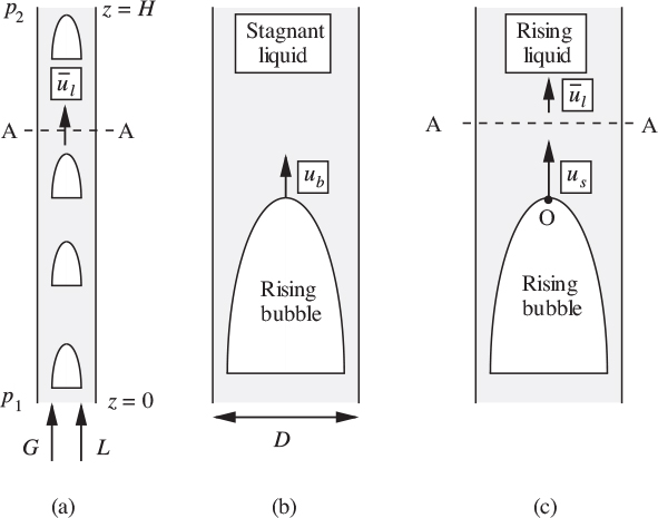
Next, consider Fig. 10.5(b), which shows a somewhat different situation—that of a single bubble, which is moving steadily upward with a rise velocity ub in an otherwise stagnant liquid. For liquids such as water and light oils that are not very viscous, the situation is one of potential flow in the liquid. Under these circumstances, Davies and Taylor used an approximate analytical solution (see Problem 10.8 to retrace their analysis) that gave11:
11 Davies and Taylor, op. cit.
in which c = 0.33 and g is the gravitational acceleration. Experimental evidence shows that the constant should be c .
The situation of Fig. 10.5(a) is now shown enlarged, in Fig. 10.5(c). The slug is no longer rising in a stagnant liquid, as in Fig. 10.5(b), but in a liquid whose mean velocity just ahead of it is ![]() . Further, near the “nose” O of the slug—at the center of the pipe, where the velocity is the highest—the liquid velocity will be somewhat larger, namely, about
. Further, near the “nose” O of the slug—at the center of the pipe, where the velocity is the highest—the liquid velocity will be somewhat larger, namely, about ![]() , as shown by Nicklin, Wilkes, and Davidson, provided that the Reynolds number between slugs exceeds 8,000.12 Therefore, the actual rise velocity of the slug is:
, as shown by Nicklin, Wilkes, and Davidson, provided that the Reynolds number between slugs exceeds 8,000.12 Therefore, the actual rise velocity of the slug is:
12 D.J. Nicklin, J.O. Wilkes, and J.F. Davidson, “Two-phase flow in vertical tubes,” Transactions of the Institution of chemical Engineers, Vol. 40, No. 1, pp. 61–68 (1962).
By conservation of the gas:
in which ε is the void fraction (the fraction of the total volume that is occupied by the gas). Hence, eliminating us between Eqns. (10.35) and (10.36):
If G and L are known, Eqn. (10.37) gives the void fraction, which is the dominant factor in determining the pressure gradient in the vertical direction:
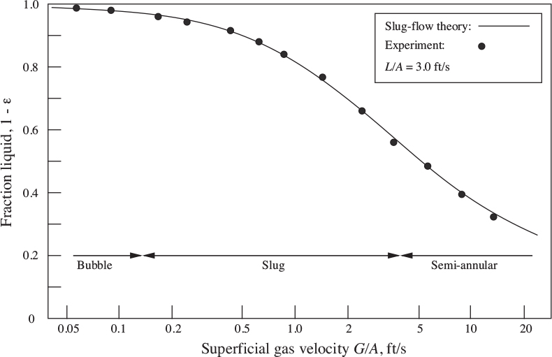
in which ρg has been neglected in comparison with ρl in the definitions of the dimensionless superficial velocities from Eqn. (10.28). Fig. 10.6 shows that the above theory is completely substantiated by experiments reported by Nicklin, Wilkes, and Davidson, not only for the complete slug-flow regime, but (somewhat unexpectedly) for the adjoining parts of the bubble- and semiannular-flow regimes as well.
Fig. 10.6. Experimental liquid void fractions for two-phase air/water flow in a vertical 1.02-in. diameter tube, as a function of the gas superficial velocity, with a liquid superficial velocity of 3.0 ft/s. From D.J. Nicklin, “Two-Phase Flow in Vertical Tubes,” Ph.D. dissertation, University of Cambridge, 1961.
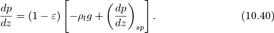
Concerning the pressure gradient, note that the density of the liquid, which occupies a fraction (1−ε) of the total volume, is much greater than that of the gas. Therefore, the pressure gradient is given to a good approximation by considering only the hydrostatic effect:
A secondary correction to (10.39) would include the wall friction on the liquid “pis-tons” between successive gas slugs. Thus, if (dp/dz)sp is the single-phase frictional pressure gradient for liquid only, flowing at a mean velocity ![]() , a more accurate expression for the pressure gradient is:
, a more accurate expression for the pressure gradient is:
The above analysis is for an ideal liquid of negligible viscosity, in which inertial and gravitational effects are dominant. White and Beardmore have investigated slug rise velocities for a wide variety of liquids and have plotted the results as Fr (the Froude number) versus Eo (the Eötvös number), with a property group Y as a parameter, where13:
13 E.T. White and R.H. Beardmore, “The velocity of rise of single cylindrical air bubbles through liquids contained in vertical tubes,” chemical Engineering Science, Vol. 17, pp. 351–361 (1962). occurs provided that the pipe diameter D > 2.26 cm. Basically, viscous effects are relatively unimportant for most low-viscosity liquids in pipes likely to be used in practice. A representative lubricant, Voluta oil (ρ = 0.902 g/ml, μ = 294 cP, σ = 30.8 g/s2, Y = 2.8) would need Eo > 3,000 to be considered ideal, which would occur for pipes with D> 10.22 cm.

For all liquids, Fr rises from zero to an asymptotic value of about 0.345 as Eo increases, but rises more slowly for larger values of Y . The authors conclude that distilled water (ρ = 0.997 g/ml, μ = 0.87 cP, σ = 71.5 g/s2, Y = 1.54 × 10⁻¹¹) behaves ideally, with Fr essentially at its full value of 0.345, for Eo > 70, which
Fig. E10.4 shows a gas-lift “pump,” in which the buoyant action of a volumetric flow rate G of gas serves to lift a volumetric flow rate L of liquid from a height H0 in a reservoir to a height H in a vertical pipe of diameter D and cross-sectional area A, in which slug flow may be assumed. Neglect liquid friction in both the supply pipe and in the vertical pipe.
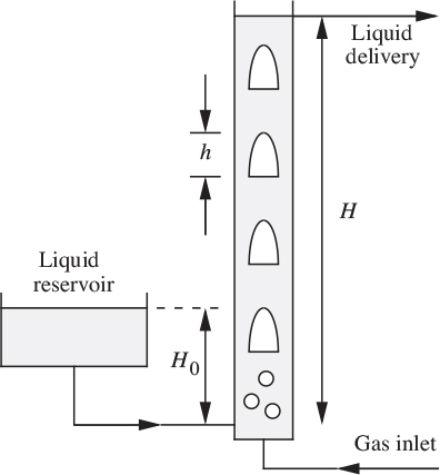
(a) Derive an expression for the void fraction ε in the column in terms of H and H0.
(b) If L = 0 (that is, the liquid is just on the verge of reaching the top), prove that the height H is given by:
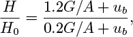
where ![]() .
.
(c) If the value of G/A is much larger than ub, what is the maximum height Hmax to which the liquid can be raised (still with L = 0)? Give your answer as a multiple of H0.
(d) If the column has a diameter D =0.1 m and operates with a positive liquid flow rate such that ε =0.5 and G/A =2L/A, what is the value of G/A (m/s)?
Solution
(a) From hydrostatics, the pressure at the base of the column is obtained in two ways:
which gives:
(b) From Eqn. (10.38), with ![]() :
:

Rearrangement and solution for the height ratio yields the desired result:
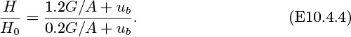
(c) For G/A≪ ub, the velocity ub in the numerator and denominator of Eqn. (E10.4.4) can be neglected, so that:

Thus, the maximum height attainable is six times the reservoir height H0.
(d) Inserting numerical values:

The superficial velocity of the gas is therefore:
which then suffices to achieve the desired liquid flow rate.
Annular flow
Consider the simultaneous flow of gas and liquid in a vertical tube as in Fig. 10.7. One approach, recommended by Wallis (op. cit.), is to use the Lockhart/Martinelli correlation for the frictional part of the pressure drop, and supplement this with appropriate gravitational terms.
Fig. 10.7. Vertical annular two-phase flow.

First, consider just the flow of gas in the inner core. Since the gas velocity vg is typically much higher than that of the liquid, the pressure gradient may be approximated as if the gas were flowing with velocity vg in a pipe of diameter Dg, giving:


in which the substitution ![]() comes from Eqns. (10.19) and (10.20).
comes from Eqns. (10.19) and (10.20).
Second, consider the entire flow, obtaining the frictional contribution from the viewpoint of the liquid:

For specified gas and liquid flow rates, the derivatives on the right-hand sides of Eqns. (10.43) and (10.44) will be known. These equations can then be solved simultaneously for the pressure gradient (dp/dz)tp and the void fraction ε. One suitable procedure involves:
(a) Equating (10.43) and (10.44), thereby eliminating (dp/dz)tp and giving a single equation with unknowns ![]() ,
, ![]() , and ε.
, and ε.
(b) Using Eqn. (10.23) to eliminate ![]() in favor of X and
in favor of X and ![]() , giving a single equation with unknowns
, giving a single equation with unknowns ![]() , X, and ε.
, X, and ε.
(c) Solving for ![]() , X, and ε by using the information in Table 10.4.
, X, and ε by using the information in Table 10.4.
Gas and oil are flowing upwards at volumetric flow rates G = 10.0, L = 0.1 ft3/s in a vertical pipeline of internal diameter D =0.25 ft. Estimate the fraction of gas, the pressure gradient, and the mean velocities of each phase. The physical properties are ρg = 0.15, ρl = 50.0 lbm/ft3, μg = 0.025, μl = 20.0 lbm/ft hr; the Fanning friction factor is fF= 0.0045.
Solution
The following quantities are first calculated:
Superficial velocities
Dimensionless superficial velocities from Eqn. (10.28)
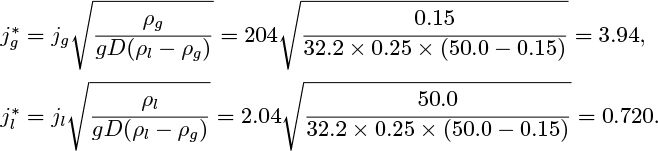
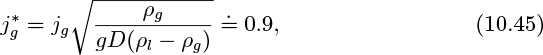
Recall that from Eqn. (10.27) that the approximate value of ![]() at which slug flow becomes annular flow is given by
at which slug flow becomes annular flow is given by ![]() . This transition value is clearly exceeded, and the flow is taken to be annular. The appropriate pressure gradients for inclusion in Eqns. (10.43) and (10.44) are:
. This transition value is clearly exceeded, and the flow is taken to be annular. The appropriate pressure gradients for inclusion in Eqns. (10.43) and (10.44) are:
Gas only

Liquid only

Reynolds numbers
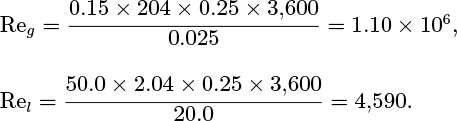
Thus, the flow is turbulent for the liquid and turbulent for the gas, with n =4.12 (from Table 10.5) for use in Eqn. (10.26). Equations (10.43) and (10.44) now become:

Now equate the two pressure gradients, substitute ![]() from Eqn. (10.23), and collect terms:
from Eqn. (10.23), and collect terms:

which can be solved in conjunction with Eqns. (10.25) and (10.26) to give:
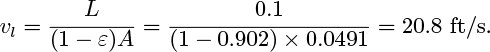
Thus, the fraction of gas is 0.902, so the oil occupies a fairly thin film on the inside of the tube. The pressure gradient is next calculated.
Two-phase flow pressure gradient

Finally, the individual mean velocities are obtained:
Gas
Liquid
10.5 Flooding
Consider two-phase flow in a vertical tube with the gas flowing upward and the liquid downward. For sufficiently high relative velocities, unstable waves will form at the gas/liquid interface, eventually resulting in fragments of liquid that break away, to be carried upward by the gas, at which stage normal countercurrent operation ceases and flooding occurs. For small liquid flow rates, Wallis (op. cit.) gives the condition under which no liquid will flow downward as:
(in which jg is the same as the gas velocity vg in Fig. 10.8), and also presents the following limiting condition for flooding in tubes with sharp-edged flanges:
Fig. 10.8. Model for flooding correlation.
with the constant rising to the range 0.88–1.00 if end effects are minimized.
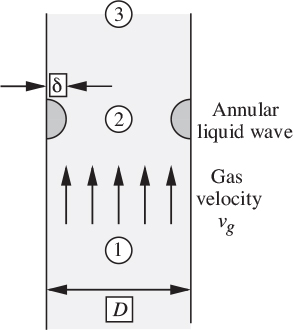
A condition remarkably close to that of Eqn. (10.45) can be derived by an elegant method suggested by Whalley and also paralleled by Problem 2.44 of the present book.14 The general idea is shown in Fig. 10.8, in which an annular-shaped “wave” with a semicircular cross section of small radius δ is supposed to have formed on the thin film lining the inner surface of the tube. The gas accelerates between locations 1 and 2, with an attendant pressure decrease from the Bernoulli effect. There is some recouping of the pressure between locations 2 and 3, but only a partial amount because of turbulence in the expanding flow.
14 P.B. Whalley, Boiling, Condensation, and Gas-Liquid Flow, Clarendon Press, Oxford, 1987.
From Eqn. (2.65), the overall pressure drop is:

in which the areas at the indicated sections are (for δ≪ D):
The area ratio and pressure drop then become:

At the onset of flooding, the pressure drop just suffices to counterbalance the weight of the wave, which has a circumference πD and a cross-sectional area πδ2/2, so that: (p1 − p3)
Elimination of (p1 − p3) from the last two equations gives, upon rearrangement:
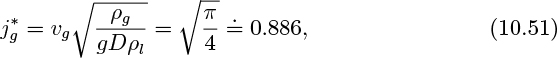
which is in essential agreement with Eqn. (10.45). Note that a different assumed shape of the wave cross section would give a somewhat different numerical value for the constant in Eqn. (10.51). However, even with some uncertainty in the value, the analysis demonstrates that ![]() is an important dimensionless group to include in any attempted correlation for flooding. Also see Problem 7.14.
is an important dimensionless group to include in any attempted correlation for flooding. Also see Problem 7.14.
Packed columns
Packed columns are used in chemical engineering for absorbing a component from a gas stream into a liquid stream, and also for conducting certain distillation operations. As shown in Fig. 10.9, the liquid is sprayed through a distributor at the top of the column and flows countercurrent to the gas, which is admitted at the bottom.
Fig. 10.9. Packed column for gas absorption.

In order to increase the surface area for mass transfer, the column is filled with inert “packing,” of which the ceramic Raschig ring is an early example. Other types of packing are Pall rings and Burl saddles, and often contain more convoluted internal surfaces.
If attempts are made to increase the gas and liquid throughputs, a stage will be reached at which the pressure drop in the vertical direction suffices to arrest the downflow of the liquid, at which stage the column fills up or “floods” with liquid, and normal operation ceases. The flooding limits are shown in Fig. 10.10, which is derived from information in an article by Eckert.15 Note that the ordinate is not dimensionless, and that the variables must have the units indicated in Table 10.6. The reader may wish to check the extent to which the ordinate is related to the dimensionless velocity in Eqn. (10.51).
15 J.S. Eckert, “Selecting the proper distillation column packing,” chemical Engineering Progress, Vol. 66, No. 3, pp. 39–44 (1970).
Fig. 10.10. Correlation for flooding in packed columns.
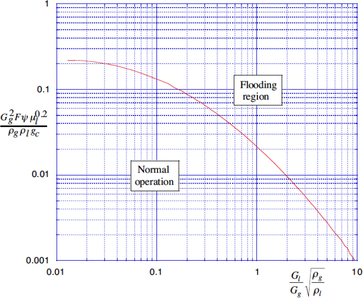
Table 10.6. Variables for Packed-Column Flooding Correlation

Representative packing factors are given in Table 10.7, and the capacity of the column is inversely proportional to the square root ![]() of the packing factor. Eckert discusses advantages and disadvantages of several packing materials. Although the smaller size packings enhance mass transfer, they have lower capacities and cost more. Nominal 2-in. packing appears optimal in most circumstances.
of the packing factor. Eckert discusses advantages and disadvantages of several packing materials. Although the smaller size packings enhance mass transfer, they have lower capacities and cost more. Nominal 2-in. packing appears optimal in most circumstances.
Table 10.7. Representative Values of the Packing Factor F

10.6 Introduction to Fluidization
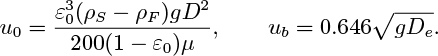
Consider the upward flow of a fluid through a bed packed with small particles. As the superficial fluid velocity u (defined as Q/A, the volumetric flow rate divided by the cross-sectional area) is increased, the behavior of the bed height h and the pressure drop Δp = p1 − p2 is shown in Fig. 10.11. A point is reached— that of incipient fluidization—when the pressure drop just suffices to support the downward weight per unit area of the bed. At this point, the superficial velocity is denoted by u0, and the void fraction by ε0 (typically between 0.4 and 0.5).
Fig. 10.11. Fluidization: (a) upward flow through a packed bed; (b) variation of bed height and pressure drop with superficial velocity.

For u>u0, the bed starts to expand and behaves essentially as a fluid; there is little subsequent increase in the pressure drop. There are two distinct modes of fluidization, depending mainly on the relative values of ρs, the density of the solid particles, and ρf , the density of the fluid.
Particulate fluidization
If ρs and ρf are of the same order of magnitude, the bed is usually a homogeneous mixture of fluid and particles. This situation occurs mainly for liquid-fluidized beds, of secondary practical importance. For u > u0, the bed expands uniformly and the void fraction obeys the Richardson-Zaki correlation16:
16 J.F. Richardson and W.N. Zaki, “Sedimentation and fluidisation,” Transactions of the Institution of chemical Engineers, Vol. 32, p. 35 (1954).
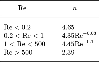
in which ut is the terminal velocity of a single particle, and the exponent n varies with the particle Reynolds number, Re = ρf udp/μf according to Table 10.8. Here, dp is the effective particle diameter and μf is the viscosity of the fluid.
Table 10.8. Values of the Richardson-Zaki Exponent
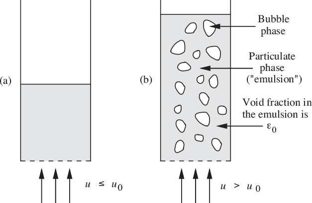
Aggregative fluidization
When the density of the fluid is considerably less than that of the particles, the bed is found to consist of two distinct phases:
1. A particulate phase or emulsion, in which the void fraction remains essentially at the incipient value ε0, even though the total fluid flow rate may considerably exceed the incipient value.
2. A bubble phase, which contains the extra fluid beyond that needed for incipient fluidization.
Aggregative fluidization occurs mainly in gas-fluidized beds, of considerable importance in industrial catalytic reactors. The general scheme is shown in Fig. 10.12. The interactive motion of the particles and bubbles will be considered in detail in Section 10.8.
Fig. 10.12. Aggregative fluidization: (a) compacted bed; (b) fluidized bed.
10.7 Bubble Mechanics
Rise velocity of a continuous swarm of small bubbles in a liquid
Paralleling the earlier discussion of gas slugs in Section 10.2, Nicklin considered the bubble regime in two-phase gas/liquid flow, again distinguishing, as shown in Fig. 10.13, between the motion of a single swarm of bubbles and of continuously generated bubbles.17 In both cases, the bubbles are produced by the passage of gas at a flow rate G through small holes in a distributor at the bottom of a column of cross-sectional area A containing a liquid.
17 D.J. Nicklin, “Two-phase bubble flow,” chemical Engineering Science, Vol. 17, pp. 693–702 (1962).
Fig. 10.13. Rise of bubbles: (a) discrete swarm, and (b) continuously generated.

Let a single cluster of bubbles rise with a velocity ub relative to the stagnant liquid above. Then, from continuity (a volume balance) on the control surface in Fig. 10.13(b), the mean upwards velocity of the liquid across X–X between two “layers” of bubbles is G/A. Hence, by the same argument used for gas slugs rising in pipes, the rise velocity uc of continuously generated bubbles is:
Note that relative to the bubbles the motion is (fairly) steady, and that liquid streamlines can be visualized. Such is not the case for a fixed observer, who will see an upflow of liquid across X–X at one instant and a downflow of liquid across X–X a moment later when a layer of bubbles has advanced to that location. If there is no net flow of liquid (it is not overflowing the column), then these two effects must cancel each other on the average.
Consider next the expansion of an initially undisturbed liquid column by bubbles flowing upward through it, with key variables defined in Table 10.9. The volumetric flow rate of gas is:
Table 10.9. Variables for Rising Groups of Bubbles
Also, the expansion of the initially undisturbed column is due to the presence of the added bubbles. Therefore, we can equate the extra volume to that of the gas:
From Eqns. (10.53)–(10.55):
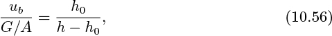
which enables ub to be deduced from experimental observations of the bed height h at different values of G/A.
Extension to a fluidized bed
The above treatment still holds for an aggregatively fluidized bed if G/A is replaced by (G/A−u0), which simply recognizes the fact that all gas above the incipient rate passes through the bed as bubbles, so the rise velocity of continuously generated bubbles is:
As an approximation (there may be a certain amount of interference between the bubbles), the rise velocity ub can be estimated from Eqn. (10.8) at the beginning of the chapter for inviscid liquids as a function of the equivalent bubble diameter De, or its equivalent in terms of the bubble volume ![]() :
:
However, for bubbles rising in fluidized-bed columns, a somewhat reduced value of the constant has been obtained instead of 0.792. The following two investigations also made the necessary corrections in order to give the rise velocities for bubbles unimpeded by walls, which can retard the bubbles if their diameter is not small compared to that of the column:
(a) Davidson et al. performed experiments in 3-in. diameter fluidized beds of glass beads and sand, with bubble volumes ranging from 5.80–15.0 ml; their results translate into a value of 0.728 for the constant.18
18 J.F. Davidson, R.C. Paul, M.J.S. Smith, and H.A. Duxbury, “The rise of bubbles in a fluidised bed,” Transactions of the Institution of chemical Engineers, Vol. 37, pp. 323–328 (1959).
(b) Harrison and Leung investigated the rise of bubbles with volumes from 25–10,000 ml in fluidized sand particles contained in a bed with a 61-cm square cross section; their results give the value of the constant as 0.712.19
19 D. Harrison and L.S. Leung, “The rate of rise of bubbles in fluidised beds,” Transactions of the Institution of chemical Engineers, Vol. 40, pp. 146–151 (1962).
Taking an average value of 0.720 for the constant, we shall use the following expressions for the bubble rise velocity:
Thus, the analog of Eqn. (10.56) for the expansion of fluidized beds is:
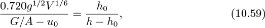
which can be used to estimate the bubble volume (and its equivalent diameter) by measuring h as a function of G/A.
Volume of a bubble formed at an orifice
Potential flow theory may also be used to determine the volume of a bubble growing and finally detaching from an orifice submerged either in a column of liquid or in an aggregatively fluidized bed.
Fig. 10.14 shows three stages in the development of an essentially spherical bubble growing at such an orifice. The volume V and radius r of the bubble keep increasing, as does the orifice-to-bubble-center-distance s = OC (this last because of buoyancy). Ultimately, s will exceed r and the bubble detaches from the orifice. The cycle then repeats, and may be analyzed as follows, after certain assumptions are made:
1. The gas volumetric flow rate G is constant. (A more complicated alternative is to consider gas supplied from a reservoir at a constant pressure, in which the flow rate fluctuates as the bubble grows and detaches.)
2. The gas is supplied by a small bore tube, and may therefore be considered as issuing from a small point. (An alternative is gas rising from a small hole in a horizontal plate, in which case none of the gas can flow downward.)
3. The gas-flow rate is neither so small that surface tension is important, nor so large that the inertia of the gas is significant (in which case a jet might form); also, viscous effects are unimportant. That is, the dominant effects are those of gravity and the acceleration of the liquid surrounding the bubble.
Fig. 10.14. Formation of a bubble at an orifice.

Since the gas flow rate is constant, the bubble volume increases linearly with time:
As the bubble rises, it accelerates the surrounding fluid. Although the bubble has essentially zero density, it has an effective mass because any bubble motion also causes the surrounding fluid (of significant density ρl) to move. The reader who solves Problem 10.4 will discover that this effective mass equals one-half of the mass of fluid displaced by the spherical bubble.
A momentum balance, equating the buoyant force to the rate of increase of effective momentum of the bubble, gives:
Elimination of V between Eqns. (10.60) and (10.61), followed by separation of variables and integration twice, yields a surprisingly simple result:
From Eqns. (10.60) and (10.65), setting r = s, the departure time is:
so that the bubble volume at detachment is:

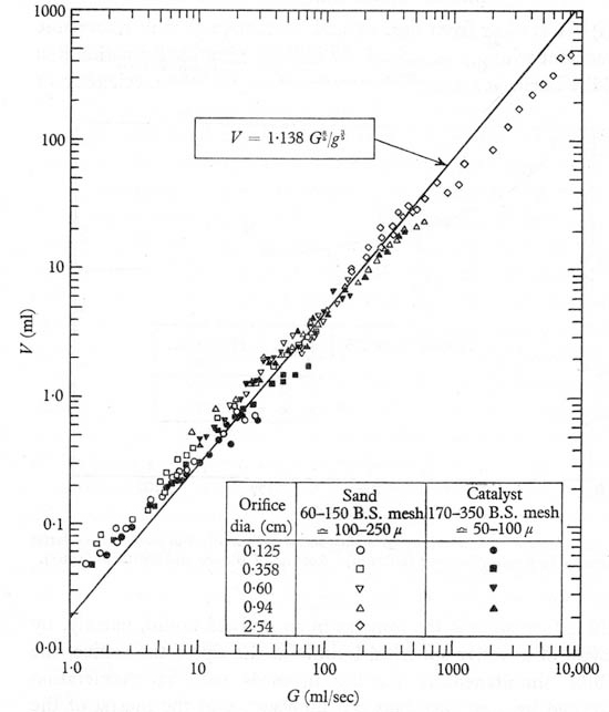
The experiments of Harrison and Leung20 and others, as reported by Davidson and Harrison21 agree well with Eqn. (10.67) under an exceptionally wide range of gas flow rates, for orifices of varying sizes situated in both liquids and fluidized beds, as shown in Fig. 10.15 for the latter. Davidson and Harrison offer several explanations for the modest deviations from theory, including: (a) bubbles not completely spherical, (b) circulating currents induced near the orifice by the train of rising bubbles, and (c) coalescence of bubbles at high gas flow rates.
21 J.F. Davidson, and D. Harrison, Fluidised Particles, Cambridge University Press, Cambridge, 1963, pp. 53, 59.
Fig. 10.15. Volumes of bubbles formed at orifices in incipiently fluidized beds. Reproduced with permission of IchemE from Harrison and Leung20.
20 D. Harrison and L.S. Leung, “Bubble formation at an orifice in a fluidised bed,” Transactions of the Institution of chemical Engineers, Vol. 39, pp. 409–414 (1961).
The treatment for an orifice located in a horizontal plate is similar, and has been studied by Davidson and Schüler.22 The effective mass of the bubble is now 11/16 times the mass of the displaced liquid, and the final result is V = 1.378 G6/5/g3/5.
22 J.F. Davidson and B.O.G. Schüler, “Bubble formation at an orifice in an inviscid liquid,” Transactions of the Institution of chemical Engineers, Vol. 38, pp. 335–342 (1960).
10.8 Bubbles in Aggregatively Fluidized Beds
The ultimate goal of this section is to examine the interaction between two gas regimes—that in the rising bubbles and that in the particulate phase—for aggregatively fluidized beds. The treatment is that of Harrison and Davidson in their 1963 book (op. cit.), which is a model of clarity and conciseness. The fluid mechanics principles involved afford a nice culmination to the previous work, especially that in Chapter 7.
Consider first the definitions shown in Table 10.10. Since both the particles and the fluidizing fluid are effectively incompressible, the continuity equation can be applied to both phases:
Fluid:
Particles:
The bed also behaves as a porous medium, so Darcy’s law applies:
Although the superficial velocity was given by d’Arcy’s law as discussed in previous sections, vf in Eqn. (10.70) is the mean interstitial fluid velocity in the interstices or spaces between the particles.
Table 10.10. Variables for a Bubble Rising in a Fluidized Bed

The fluid and particle velocity vectors may be eliminated from Eqns. (10.68)– (10.70), yielding a simple and familiar result:
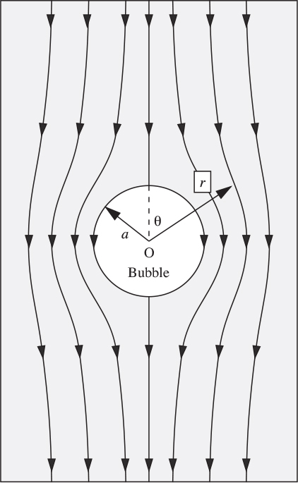
That is, the pressure distribution obeys Laplace’s equation, and is independent of the particle motion. Representative isobars are shown in Fig. 10.16, where, for simplicity, a rising spherical bubble is assumed to be at the midpoint between high- and low-pressure regions of pressure p = ±P , separated by a distance 2h. The coordinates are such that r = 0 is at the center of the bubble, and θ is measured downward from the vertical. The reader may check that the following pressure distribution satisfies Eqn. (10.71) and the boundary conditions at the top and bottom of the bed, and on the surface of the bubble:

Fig. 10.16. Isobars in the vicinity of the bubble.
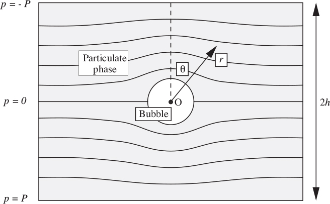
in which the overall pressure gradient well away from the bubble is:
In catalytic reactors, it may be important to know the volumetric flow rate Q of the fluidizing fluid that is entering the lower hemisphere of the bubble and departing from its upper hemisphere. The development outlined in Problem 10.5 shows that by integrating over one of these hemispheres,
Since the upward superficial fluid velocity well away from the bubble is u0, Eqn. (10.74) shows that the cavity—and reduced resistance—caused by the bubble attracts three times the normal fluid flow rate.
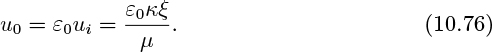
Well away from the bubble, the interstitial fluid velocity ui relative to the particles is in the vertically upward direction and obeys d’Arcy’s law:
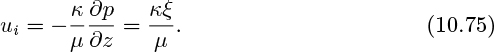
The superficial velocity at incipient fluidization, which is based on the total cross-sectional area—not the restricted area between the particles—will be lower, equaling the void fraction times the relative interstitial velocity:
Motion of the particles
For an observer moving upwards with a bubble, the velocity potential for the streaming motion of the particles is obtained from Eqn. (7.73):
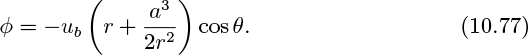
The corresponding streamlines are shown in Fig. 10.17.
Fig. 10.17. Downward streaming of particles past a bubble.
Motion of the fluidizing fluid
The individual velocity components for the fluidizing fluid are again obtained from d’Arcy’s law, Eqn. (10.70):

in which the particle velocity components are given by:
where the velocity potential ϕ has already been given in Eqn. (10.77).
Fig. 10.18. Bubble rise velocity ub is less than the incipient interstitial fluidizing velocity ui.

From Eqns. (10.72), (10.75), and (10.77)–(10.80), the fluid velocities are therefore:


The flow pattern of the fluid may be traced by examining its stream function:
Fig. 10.19. Bubble rise velocity ub is greater than the incipient interstitial fluidizing velocity ui.

The following solution is consistent with Eqns. (10.81)–(10.84):

in which

The corresponding streamlines for both the fluid and the particles are presented in Figs. 10.18 and 10.19, relative to an observer traveling upward with the bubble. Although in both cases the particles “rain down” around the bubble identically, there are two quite distinct flow regimes as far as the fluidizing fluid is concerned:
1. For ub < ui, the bubble rise velocity is less than the incipient interstitial fluidizing velocity. Generally, there is an excellent interchange of fluid between the bubble and the more remote parts of the fluidized bed, with a relatively small “recycle” of fluid back to the bubble.
2. For ub >ui, the bubble rise velocity exceeds the incipient interstitial fluidizing velocity. The interchange of fluid between the bubble and the particles is now confined to a relatively small zone in the immediate vicinity of the bubble. All fluid within a sphere of radius α continuously recirculates in and out of the bubble; this is apparent from Eqn. (10.85), which, for r > α, represents streaming around a sphere of radius α.
When the gas stream contains reactive components whose reaction is catalyzed by the particles, the performance of the bed as a reactor may be predicted from relatively simple extensions of the above theory, as illustrated by the following example. The works of Orcutt, Davidson, and Pigford, on the decomposition of ozone, and Harrison and Davidson (op. cit.), who discuss several different reactions, are recommended for further information.23
23 J.C. Orcutt, J.F. Davidson, and R.L. Pigford, “Reaction time distributions in fluidized catalytic reactors,” chemical Engineering Progress Symposium Series, Vol. 58, No. 38, pp. 1–15 (1962).
The particle bed in Fig. E10.6 contains uniform bubbles of volume V when fluidized at a superficial velocity U by gas that contains a small entering concentration c0 of a reactant, which decomposes rapidly on contact with the particles.
Show that the exit concentration at the top of the bed is given by:
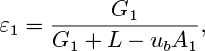
where X = Qh/ucV , u0 is the incipient fluidizing velocity, Q is the volumetric cross-flow rate between a bubble and the particulate phase, h is the bed height, and uc is the absolute velocity of the continuously generated bubbles.
Use these results to estimate ce/c0 for a bed of large diameter containing bubbles of equivalent diameter De = 0.15 m, where ![]() . Take u0 = 0.2 m/s, U = G/A =1.5 m/s, and h0 (the height of the bed at incipient fluidization) =0.5 m. The bubble-rise velocity is
. Take u0 = 0.2 m/s, U = G/A =1.5 m/s, and h0 (the height of the bed at incipient fluidization) =0.5 m. The bubble-rise velocity is ![]() .
.
Solution
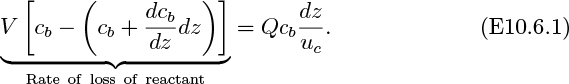
Consider a single bubble rising a distance dz—which it will traverse in a time dz/uc—with the concentration of reactant changing from cb to cb +(dcb/dz)dz. The rate of loss of reactant due to recirculation out of the bubble is Qcb; since the reaction is virtually instantaneous in the emulsion phase, no reactant enters the bubble. A mass balance on the bubble gives:
Separation of variables and integration between the inlet and exit, where the concentration in the bubbles is cbh, gives:

Fig. E10.6. Reacting gas rising in a fluidized bed.
Since the entering superficial velocity is U and that needed for incipient fluidization is only u0, the fraction of entering gas passing through as bubbles is (U − u0)/U = 1 − u0/U. Also, the gas passing through in the emulsion phase reacts quickly and contributes nothing to the reactant concentration at the exit. Thus, the net reactant concentration at the exit is given by:
The cross-flow rate in and out of the bubbles for a spherical bubble of radius a is given by Eqn. (10.74):
(In some situations, this flow rate may be enhanced by diffusion of gas from the bubble to the surrounding particles, but this effect is neglected here.)
The height h of the bed after it has expanded from its incipient value h0 can be obtained from Eqn. (10.59), recognizing that G/A = U:

All necessary quantities can now be calculated:
Bed height
Bubble rise velocity
Bubble volume
Cross flow rate
Fraction of reactant in the exiting gas stream

For finite reaction rates in the bed, two fruitful avenues are available, as discussed by Orcutt et al. (op. cit.) and Davidson and Harrison (op. cit.):
1. Treat the particulate phase as well-mixed, with a single concentration throughout, in which case an overall balance for the reacting species can be performed on the bed.
2. Consider the concentration in the particulate phase as a function of elevation z, in which case a differential balance must be performed for the reacting species in the bed.
Problems for Chapter 10
Unless otherwise stated, all flows are steady state, with constant density and viscosity.
1. Gas slug between parallel plates—D (C). Fig. P10.1 shows the cross section through a large bubble OPQ between two parallel vertical plates AA and BB that are separated by a distance 2a. For purposes of experimental observation, the bubble is held stationary by a downward flow of an inviscid liquid whose velocity is U far upstream of the bubble. The motion is two-dimensional, so that the flow pattern is the same in all planes parallel to that of the diagram.
Fig. P10.1. Flow downward past a stationary gas bubble.

The following approximate relation has been proposed for the stream function in the liquid:
Verify that this stream function satisfies:
(a) Laplace’s equation.
(b) The boundary condition far above the bubble.
(c) The boundary conditions along the walls AA and BB.
Prove that for small values of y, the equation for the free surface OPQ is:
What boundary condition must be satisfied along this free surface? Show that if this boundary condition is satisfied for small values of y, then the bubble-rise velocity in an otherwise stagnant liquid is:
2. Pressure drop in slug flow—M. A light oil and a gas are flowing upward in a vertical tube of 4.0-in. I.D. at superficial velocities of L/A = 1.2 ft/sec and G/A =4.8 ft/sec, respectively. The viscosities of the oil and gas are 15.6 and 0.038 lbm/ft hr, respectively; their densities are 48 and 0.42 lbm/ft3.
Assuming commercial steel pipe (fF= 0.00675) with slug flow prevailing, calculate the pressure drop (psi) in the pipe for every 10 ft of vertical rise.

3. Gas-lift pump—M. Fig. P10.3 shows a gas-lift “pump,” in which the buoyant action of a volumetric flow rate G of gas serves to lift a liquid from a height H0 to a height H above the bottom of a vertical pipe of diameter D and cross-sectional area A. Analyze the most favorable case with L = 0—that is, with no net liquid flow:
(a) Assuming slug flow of the gas, what superficial gas velocity G/A is then needed to “expand” the liquid column from an initial height H0 to a final height H? Take H0 = 20 ft, H = 60 ft, and D = 3 in.
(b) What is the maximum upward liquid velocity, and where does it occur?
(c) What is then the maximum downward liquid velocity, and where does it occur? (On the average, the slug length is 2 ft.)
(d) To a first approximation, what gas inlet pressure (psig) is needed if the liquid is water?
4. Potential flow around a bubble—M. This problem is closely related to Section 10.7, concerning the volume of bubbles produced at an orifice. Consider a spherical bubble of radius a moving upward with a velocity ub in an inviscid liquid. Relative to a stationary observer, what is the justification for supposing that the potential function for the flow of the liquid is:
As long as the circumstances are explained properly, you may quote any equation in the chapter in order to arrive at your conclusion.
Next, prove that the magnitude u of the velocity at any point (r, θ) in the liquid is given by:

Finally, consider the total kinetic energy of the liquid surrounding the bubble:
where dm is a differential element of mass, and prove that this equals half the kinetic energy of a sphere of radius a and density equal to that of the liquid. In other words, prove that the effective mass of the surrounding fluid is one half of the mass displaced by the spherical bubble.
Fig. P10.5. Geometry for gas passing through a bubble.

5. Gas percolation through a bubble—M. Fig. P10.5 shows a detailed view of a single bubble at the midpoint of an aggregatively fluidized bed, as in Fig. 10.16. Arrows represent the gas flow entering the lower hemisphere; a similar flow rate of gas departs from the upper hemisphere, although (to avoid confusion) the arrows are omitted in this case.
Following the notation of Section 10.8, consider the radial pressure gradient at the surface of the bubble, r = a. By integration over one of the hemispheres, verify Eqn. (10.74) for the flow rate of gas from the bed through the bubble:
6. Pressure distribution in a fluidized bed—M. For a fluidized bed, check that the continuity equations for the fluid and particles, when combined with d’Arcy’s law, lead to Laplace’s equation, (10.71), for the pressure. Then verify that the proposed pressure distribution from Eqn. (10.72) for the situation shown in Fig. 10.16 satisfies:
(a) Laplace’s equation.
(b) The condition that p = 0 at the bubble surface.
(c) The conditions that p = ±P at the bottom and top of the bed, respectively.
7. Stream function in a fluidized bed—M. Consider the motion of the fluid in a fluidized bed. Starting from Eqns. (10.78) and (10.79), verify the relations given in Eqns. (10.81) and (10.82) for the velocity components ![]() and
and ![]() . Then prove the relations given in Eqns. (10.85) and (10.86) for the fluid stream function.
. Then prove the relations given in Eqns. (10.85) and (10.86) for the fluid stream function.
8. Slug flow in a tube—D. This problem parallels the work of Davies and Taylor for determining the rise velocity ub of a gas slug or bubble ascending in an otherwise stagnant inviscid liquid in a vertical tube of radius a.24 By superimposing a downward velocity ub on the system, the analysis is performed for liquid streaming downward past a stationary bubble, as shown in Fig. P10.8.
24 R.M. Davies and G.I. Taylor, “The mechanics of large bubbles rising through extended liquids and through liquids in tubes,” Proceedings of the Royal Society, Vol. 200A, pp. 375–390 (1950).
Fig. P10.8. Gas slug in a tube.

The following relationships may be assumed for the velocities, potential function, and stream function in the coordinate system shown, with symmetry about the z axis:
The following forms are assumed for the potential and stream functions:
Also, note that the solution of the differential equation,

is given by y = Jn(x), the nth-order Bessel function of the first kind. The following relations may be needed:
Development. With the above in mind, verify the following:
(a) By substituting for ϕ and ψ from Eqns. (P10.8.3) into Eqns. (P10.8.2), check that:

Thus, the potential and stream functions are now:

(b) Derive expressions for vr and vz from both ϕ and ψ, and make sure that both approaches agree with each other. Far above the nose of the bubble, show that the velocity is uniformly ub downward.
(c) Since there is no radial velocity component at the tube wall, check that:
an equation whose lowest root you can assume is k =3.832. (There are additional roots, such as the nth-order root kn, so more terms such as AnJ0(knr/a) could be included for the potential function, but we are only considering the simplest case here.)
(d) Along r = 0, the centerline above the nose of the bubble at the origin O, verify that the stream function is zero (and continues this value along the surface of the bubble to points such as P and Q). Prove that the wall (r = a) is also a streamline, whose value of ψ corresponds to a flow rate through the tube of πa2ub.
(e) At the stagnation point O, check that vr = 0 is immediately satisfied. Also prove that the requirement that vz is also zero there leads to:
(f) Note that because of the gas in the bubble, the pressure is uniform along OPQ, so that the Bernoulli condition along the bubble surface is:
With only a single term in the approximation for ϕ, this condition can only be observed at a single point, which we shall take at r = a/2. By considering the streamline ψ = 0, and assuming that J1(3.832/2) = 0.580, show that this occurs when z/a = 0.131. Also assuming that J0(3.832/2) = 0.273, verify that the Bernoulli condition leads to the relation:
where D is the tube diameter. What are the values for the constants c1 and c2?
9. Performance of a bubble reactor—M. Fig. P10.9 shows a bubble reactor, which uses air bubbles both for removing a trace of bacteria from water and for generating a circulation of water down a central tube of length H and up the surrounding annulus, each of which has the same cross-sectional area A. The air is injected as bubbles at a volumetric flow rate G at a height h above the bottom of the tube, and eventually disengages at the top of the annulus.
The diameter of the bubbles, which may be assumed constant, is such that a discrete swarm of the bubbles (not continuously generated) would rise with velocity ub in stagnant water. Answer the following, using any or all of the variables A, g, G, h, H, L, and ub:
(a) In terms of A, G, L, and ub, give expressions for the absolute velocities of the bubbles that are continuously generated: uct downward in the tube and uca upward in the annulus. Bear in mind that there are net flows of both the gas (G) and liquid (L).
(b) Still bearing in mind that the total air flow rate is G, derive expressions for the void fractions—εt in the tube and εa in the annulus, in terms of A, G, L, and ub.
(c) If the total head loss due to the fluid circulation is c(L/A)2, where c is a constant, prove that:

Hint: Cycle around from any starting point in the loop, such as the gas injection nozzles, and note that the net pressure change must equal zero when the starting point is again reached. Pressure and head changes are related by Δp = ρgΔh.
(d) If G/A =0.1 m/s, H =10 m, h =5 m, L/A =0.9 m/s, and ub =0.25 m/s, calculate the values of εt, εa, and c, and give the units for c.
(e) How would you recommend starting up the reactor?

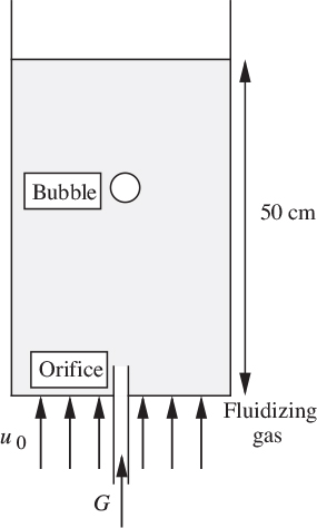
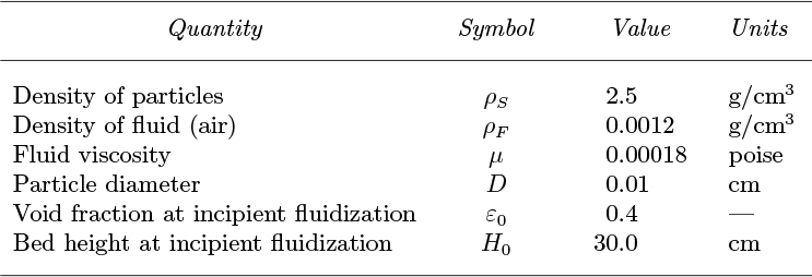
10. Bubble motion in a fluidized bed—M. An experimental aggregatively fluidized bed is operated with an incipient superficial velocity of u0 = 10 cm/s, and the corresponding void fraction is ε0 = 0.45. As shown in Fig. P10.10, a single spherical bubble is generated from the orifice by a gas flow rate of G = 100 cm3/s, after which the gas flow is abruptly terminated. If needed, g = 981 cm/s2.
Now answer the following questions:
(a) Verify that the volume of the bubble is approximately 4.58 cm3. What is its diameter (cm)?
(b) Assuming that it is quickly reached, what is the steady upward rise velocity of the bubble (cm/s)? How long (s) does it take for the bubble to reach the top of the bed after leaving the orifice?
(c) During this period, how much gas enters and leaves the bubble (expressed as a multiple of the bubble volume?
(d) Is the entering gas in (c) essentially fresh gas from the rest of the bed, or is it mainly gas that is recycled from the bubble itself?
Fig. P10.10. Bubble rising in a fluidized bed.
11. Flow of expanding gas slugs—D. Consider the case of slug flow in a vertical pipe of diameter D and cross-sectional area A, with no net liquid flow. The height H of the pipe is substantial, so the bubbles expand as they rise toward the top of the pipe, where the pressure is pT and the gas density is ρgT . Assuming isothermal ideal-gas behavior with negligible wall friction, prove that the necessary pressure at the bottom of the pipe is:

Here, ρl is the liquid density, m is the mass flow rate of gas, and ![]() is the rise velocity of a single slug in a stagnant liquid.
is the rise velocity of a single slug in a stagnant liquid.
12. Bubble rise in a fluidized bed—M (C). The superficial velocity of air needed for incipient fluidization of a bed of catalyst particles is 5.4 cm/s, and the mean bed depth is then 22.2 cm. At higher air velocities, the bed consists of a dense phase, together with bubbles that all have the same equivalent diameter, De.
Estimate De when the superficial air velocity is 28.4 cm/s and the mean bed height is 41.5 cm. How long do the bubbles take to rise through the bed, and what proportion of the air passing through the bed do they represent? What is the mean residence time for the air in the dense phase?
Assume that the void fraction of the dense phase remains constant at 0.4, the value at incipient fluidization.
13. Fluidized-bed residence time—D (C). Explain the importance of the incipient fluidizing velocity u0, and the bubble-rise velocity ub, in understanding the behavior of an aggregatively fluidized bed. Outline the steps in the derivation of the following results:
A shot of gaseous tracer is suddenly injected into the base of an air fluidized bed of spherical particles. Calculate the mean residence time of the tracer when the superficial velocity U = u0. When U = 10 cm/s, the mean bubble diameter De may be taken as 2 cm; estimate the time for the first tracer material to appear at the top of the bed. Show on a sketch how the outlet concentration of tracer varies with time after injection. Use the values given in Table P10.13.
Table P10.13. Data and Notation
14. U-tube bubble reactor—M. Fig. P10.14 shows a bubble reactor of height H, in which volumetric flow rates G1 and G2 of gas are injected at the top of the downcomer and at the base of the riser, respectively. The cross-sectional areas, void fractions, and absolute gas-bubble velocities are denoted by A, ε, and uc, with subscripts 1 and 2 referring to the downcomer and riser, respectively. The volumetric liquid circulation rate is L. All injected bubbles leave at the top of the riser.
Prove that the void fraction in the downcomer is:
in which ub is the rise velocity of a discrete swarm of bubbles relative to stagnant liquid. Obtain the corresponding expression for ε2 in the riser.
Fig. P10.14. Reactor with double gas injection.
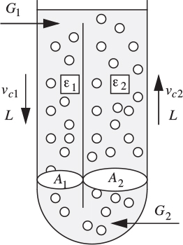
The frictional head loss per unit depth is found experimentally to be c times the square of the corresponding superficial liquid velocity, where c =0.0452 s2/m2. If A1 =0.02, A2 =0.1m2, G1 =0.01, G2 =0.05 m3/s, and ub =0.25 m/s, calculate ε1, ε2, and L (m3/s).
15. Two-phase horizontal flow—M. Consider Example 10.2, with the sole change that the liquid volumetric flow rate is reduced to L =0.025 ft3/s. Calculate the new values of X, ϕg, ε, and (dp/dz)tp. Any values reused from Example 10.2 may be quoted without recalculating them. Note: for laminar pipe flow, fF= 16/Re.
16. Bubble diameter in a fluidized bed—D(C). Define the two-phase theory of gas fluidization, and describe briefly how it is applied in practice.
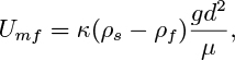
Use the theory to show that:
for a gas-fluidized bed, where u0 and h0 are the superficial gas velocity and bed height at incipient fluidization, h is the bed height at a gas velocity U, and De is the equivalent bubble diameter in the bed. State any assumptions that you make.
For a bed of spherical catalyst particles of diameter dp =0.03 cm and density ρp =2.6 g/cm3 fluidized by air, the bed height is 24.2 cm at incipient fluidization. At U =1.5u0 the mean bed height is observed to be 30.6 cm. For air: ρf =0.00121 g/cm3, μf = 0.0183 cP. Estimate the equivalent bubble diameter at this higher gas flow rate.
Use the Ergun equation for packed beds:

in which ε0 is the void fraction at the point of incipient fluidization, as distinct from the fraction of the expanded bed that is occupied by bubbles. To determine ε0, assume that the spherical particles are touching one another in a cubic manner.
17. Particulate fluidization—M (C). What is the difference between particulate and aggregative fluidization? The following results were obtained for the expansion of a bed of ball bearings by a fluid:

The free-fall velocity of a single ball bearing through the fluid is 96.0 cm/s.
Show that these results obey the Richardson and Zaki correlation, and evaluate the corresponding index. Find also the minimum fluidizing velocity, Umf , if the void fraction is 0.4 at minimum fluidization.
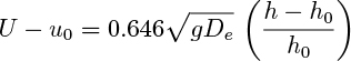
Indicate how Stokes’ law, F =3πμUd, can be used in conjunction with these results to show that:
and evaluate the constant κ. In these expressions, F is the drag force on a single particle, ρs and ρf are the densities of the solid and fluid, respectively, μ is the viscosity of the fluid, and d is the diameter of the particles.
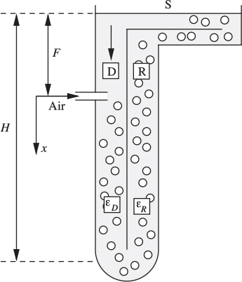
18. Aerated treatment of sewage—D (C). Fig. P10.18 shows a “deep-shaft” unit for treating sewage. The shaft (much deeper than indicated here) is partitioned into two sections D and R of equal area. Air is injected into the downcomer at a depth F . The bubbles are carried down to the bottom, up the riser R, and are then separated at S so that clear liquid returns to D. This direction of circulation is established by a start-up air supply (not shown) in R, which is turned off during normal operation.
Assume: (a) void fractions εD,εR≪ 1; (b) constant bubble-rise velocity ub relative to the liquid; (c) negligible bubble absorption; (d) in calculating the change of bubble volume, the pressure at position x is p0 +ρlgx, in which p0 is the absolute pressure at x = 0, and ρl is the liquid density.
Show that at a given x, εR/εD = (w − ub)/(w + ub), where w is the liquid velocity, and that the liquid head ΔH available to overcome friction and other hydraulic losses in the circuit is given by: ΔH εD0H0

where ρlgH0 = p0, and εD = εD0 at x =0.
Fig. P10.18. Deep-shaft aeration of sewage.
19. Slug flow fluidized-bed reactor—M (C). Consider a fluidized-bed reactor identical to that in Example 10.6, except that it now occurs in a tube of diameter D operating in the slug flow mode. The slugs have a uniform volume V and rise with an absolute velocity ub. The superficial velocity is again U and the incipient fluidizing velocity is u0; the bed height is h0 when compacted and h when fluidized.
If diffusion is negligible, outline the arguments leading to a volumetric cross flow rate Q = πD2u0/4.
Estimate ce/c0 for a bed in a tube of diameter D = 0.07 m, with De = 0.15 m. h0 = 0.5 m, u0 = 0.2 m/s, and U = 1.5 m/s. Take ![]() . The result of Eqn. (E10.6.3) may be assumed.
. The result of Eqn. (E10.6.3) may be assumed.
20. Bubble formation in a viscous liquid—M. This problem is based on investigations of Davidson and Schüler.25 Consider the growth of a single spherical bubble at an orifice in a liquid of significant kinematic viscosity ν. If the gas flow rate G is sufficiently small so that: (a) inertial effects in the liquid can be ignored, and (b) the velocity of the bubble is always at its Stokes value, prove that the bubble volume on detachment is:
25 J.F. Davidson and B.O.G. Schüler, “Bubble formation at an orifice in a viscous liquid,” Transactions of the Institution of chemical Engineers, Vol. 38, pp. 144–154 (1960).
21. Group used in flooding correlation—E. Investigate the extent to which the ordinate ![]() of Fig. 10.10 is related to the dimensionless velocity
of Fig. 10.10 is related to the dimensionless velocity ![]() in Eqn. (10.51).
in Eqn. (10.51).
22. Well-mixed fluidized-bed reactor—D. Consider the situation of Example 10.6, but now with a first-order reaction with rate constant k in the particulate phase, which is assumed to be well mixed, with a uniform reactant concentration cp.
(a) Using the same notation as in Example 10.6, prove that the reactant concentration cb in the bubble at height z above the inlet is:
(b) Explain briefly why the total rate of addition of reactant from the bubbles to the particulate phase over the entire bed equals:

where N is the number of bubbles per unit volume and A is the bed cross-sectional area.
(c) Also perform a material balance for the reactant in the particulate phase of the entire bed, and prove that:
in which the void fraction is given by ε = NV , and u0 is the incipient fluidizing velocity. Hence, determine an expression for the fraction of the reactant leaving the bed unconverted.
23. Cylindrical bubble in fluidized bed—M. Experimental fluidized beds are sometimes operated as shown in Fig. P10.23, with a cylindrical bubble rising between two transparent parallel plates, because the bubble can be photographed easily. Analyze the fluid mechanics surrounding such a bubble that is halfway up the bed, as in Fig. 10.16.
(a) Prove that the following pressure distribution in the particulate phase satisfies the appropriate Laplace’s equation:
(b) If the velocity potential for the streaming of the particles around the bubble is:

derive expressions for the particle velocity components vpr and vpθ.
(c) Finally, obtain expressions for the velocity components vfr and vfθ of the fluidizing fluid, and the stream function ψ, in terms of r, θ, a, ub, and ui.
Fig. P10.23. Cylindrical bubble rising in a fluidized bed.

24. Two-phase bubble flow—E. Consider two-phase gas/liquid flow in a vertical column of cross-sectional area 100 cm2. The rise velocity of the bubbles relative to a stagnant liquid above them is 25 cm/s. The regime is thought to be that of bubble flow.
(a) If the upward gas and liquid volumetric flow rates are G = 250 cm3/s and L = 0, respectively, what is the void fraction, and is this likely to correspond to bubble flow? If the liquid is water, and the gas density is negligible, and the height of the two-phase mixture is 100 cm, what is the pressure drop in Pa across the column? If the gas is turned off, to what height does the liquid settle?
(b) For G = L = 250 cm3/s, both upward, what is the void fraction?
(c) For G = 200 cm3/s upward, is it possible to adjust the liquid flow rate L to achieve a void fraction of ε = 0.08? If so, what is the value of L? If not, explain why such a void fraction is impossible.
25. Two-phase vertical annular flow—M. Consider Example 10.5, with the sole change that the gas volumetric flow rate is reduced to G =5.0 ft3/s.
Calculate the new values for X, ε, ϕg, and (dp/dz)tp. Any values reused from Example 10.5 may be quoted without recalculating them.
26. True/false. check true or false, as appropriate:
(a) The rise velocity of a spherical-cap bubble can be determined fairly accurately from potential-flow theory.
T ![]() F
F ![]()
(b) The equivalent diameter of a spherical-cap bubble is defined as the diameter of a sphere that has the same surface area as the bubble.
T ![]() F
F ![]()
(c) For two-phase gas/liquid flow in vertical tubes, the bubble-flow regime occurs at low gas flow rates.
T ![]() F
F ![]()
(d) The void fraction in the slug flow regime of two-phase flow in vertical tubes is important because it is a key factor in determining the overall pressure drop.
T ![]() F
F ![]()
(e) The rise velocity of a single gas slug in a tube containing a stagnant liquid above it is approximately ![]() where D is the internal tube diameter.
where D is the internal tube diameter.
T ![]() F
F ![]()
(f) Particulate fluidization occurs when excess gas— beyond that needed to effect the fluidization—travels as discrete bubbles.
T ![]() F
F ![]()
(g) In a liquid, the rise velocity of continuously generated bubbles is less than that of a single swarm of bubbles.
T ![]() F
F ![]()
(h) A fluidized bed of particles behaves almost as though it were an inviscid liquid.
T ![]() F
F ![]()
(i) A bubble, formed at an orifice in a liquid, detaches when the distance from its center to the orifice just exceeds the radius of the bubble.
T ![]() F
F ![]()
(j) The pressure in a fluidized bed obeys Laplace’s equation.
T ![]() F
F ![]()
(k) A spherical bubble cavity in a fluidized bed causes three times the normal gas flow rate to flow through it.
T ![]() F
F ![]()
(l) For a single bubble in an aggregatively fluidized bed, the nature of the motion of the particles around the bubble depends on whether or not the bubble rise velocity exceeds the incipient interstitial fluidizing velocity.
T ![]() F
F ![]()
(m) In vertical two-phase slug flow, the highest downward liquid velocity occurs in the liquid film at the base of each slug.
T ![]() F
F ![]()
(n) In the bubble reactor problem—P10.9—the reactor can be started with a fast initial air flow rate; throttling it back then gives the desired circulation.
T ![]() F
F ![]()
(o) The volume of a bubble generated at an orifice in a low-viscosity liquid depends almost entirely on the gas flow rate and the acceleration of gravity.
T ![]() F
F ![]()
(p) A single bubble rising in a fluidized bed will have more gas recycled back to itself the slower it goes.
T ![]() F
F ![]()
(q) For vertical two-phase gas/liquid slug flow in a pipe, the maximum upward liquid velocity occurs about halfway between successive gas slugs.
T ![]() F
F ![]()
(r) For vertical two-phase gas/liquid slug flow in a pipe of known diameter, a knowledge of the gas and liquid flow rates will enable the void fraction to be predicted.
T ![]() F
F ![]()
(s) For vertical two-phase gas/liquid slug flow in a pipe with zero net liquid flow, a succession of continuously generated gas slugs will rise more slowly than a single slug would in an otherwise stagnant liquid.
T ![]() F
F ![]()
(t) The rise velocities of single bubbles in a liquid increase monotonically as the bubble volume increases.
T ![]() F
F ![]()
(u) The Lockhart and Martinelli two-phase pressuregradient correlation explicitly recognizes flow regimes such as bubble flow, slug flow, and annular flow.
T ![]() F
F ![]()
(v) For two-phase gas/liquid flow in vertical tubes, the transition between slug and annular flow is well defined.
T ![]() F
F ![]()
(w) One model for predicting the onset of flooding depends on Bernoulli’s equation for determining the pressure drop as rising gas accelerates between liquid waves.
T ![]() F
F ![]()
(x) For two-phase gas/liquid bubble flow in a vertical tube, a solution cannot exist for gas downflow and liquid upflow.
T ![]() F
F ![]()
(y) The Eötvös number is a measure of the ratio of gravitational forces to viscous forces.
T ![]() F
F ![]()
(z) Although the Lockhart/Martinelli correlation was originally developed for two-phase flow in horizontal tubes, it can be used to predict the frictional part of the pressure drop for two-phase flow in vertical tubes.
T ![]() F
F ![]()