1
Formation Kinematics
This chapter introduces the notation to be used in the book, as well as the subject of vectorial kinematics, which is frequently used to derive equations of motion.
1.1 Notation
|
|
tends (or converges) to |
|
|
implies |
|
|
identically equals (or equal) |
|
|
defined as |
|
|
much smaller than |
|
|
much greater than |
|
|
for all |
|
|
(if) there exists |
|
|
belongs to |
|
|
does not belong to |
|
|
a strict subset of |
|
|
a subset of |
|
|
intersection |
|
|
union |
|
|
empty set |
|
|
maps to |
|
|
summation |
|
|
left product |
|
|
Kronecker product |
|
|
positive infinity |
|
|
set of real numbers |
|
|
set of |
|
|
set of |
|
|
set of complex numbers |
|
|
set of |
|
|
set of complex numbers with positive real parts |
|
|
set of complex numbers with negative real parts |
|
|
open ball centered at |
|
|
amplitude (or absolute value) of number |
|
|
real part of number |
|
|
imaginary part of number |
|
|
transpose of a real vector |
|
|
2‐norm of a real vector |
|
|
|
|
|
transpose of a real matrix |
|
|
induced 2‐norm of a real matrix |
|
|
induced |
|
|
the determinant of a square matrix |
|
|
a positive matrix |
|
|
a nonnegative matrix |
|
|
exponential of a real or complex number |
|
|
exponential of a real matrix |
|
|
spectral radius of matrix |
|
|
the |
|
|
the maximum eigenvalue of a real symmetric matrix |
|
|
the minimum eigenvalue of a real symmetric matrix |
|
|
rank of matrix |
| diag |
a diagonal matrix with diagonal entries |
| diag |
a block diagonal matrix with diagonal blocks |
|
|
maximum |
|
|
minimum |
|
|
supremum, the least upper bound |
|
|
infimum, the greatest lower bound |
|
|
sine function |
|
|
cosine function |
|
|
signum function |
|
|
tangent hyperbolic function |
|
|
tangent hyperbolic function |
|
|
|
|
|
|
|
|
|
|
|
imaginary unit |
|
|
|
1.2 Vectorial Kinematics
The motion of an individual vehicle, is a six degree‐of‐freedom movement in space with respect to time. If we borrow the concept of rigid‐body dynamic behaviour, such movement is often captured by a translational movement of a mass point (e.g. the centre of mass) and a rotational movement about an instantaneous axis through that point. Therefore, a distinctive description of translational or rotational dynamic behaviour is often developed through vectorial kinematics and dynamics.
1.2.1 Frame Rotation
It is essential to know how to deal with several reference frames and the transformation of the matrix representations of a vector (since the representation depends on the specific reference frame) from one frame to another. Only relative rotation (orientation change) between reference frames is important when considering representation of vectors. The relative translation does not affect the components of a vector since neither direction nor magnitude depends on the placement of the frame's origin. Translational motion between frames can be treated in the same way as Galilean transformation.
The physical description of motion of a mass point requires an origin to construct a vector. It is different from the general statement of independence of a vector from a reference frame origin.
Rotation Matrix
A vector ![]() has different expressions under two different frames
has different expressions under two different frames ![]() and
and ![]() :
:
where ![]() and
and ![]() are numerical expressions of vector
are numerical expressions of vector ![]() under frames
under frames ![]() and
and ![]() respectively, sometimes referred to as numerical vectors. The vector‐like
respectively, sometimes referred to as numerical vectors. The vector‐like ![]() and
and ![]() are vectorized representations of frame axes,
are vectorized representations of frame axes, ![]() ,
, ![]() . We simply call these vectrices, a made‐up name for axis vectors presented in matrix format. It is obvious that the relationship between two expressions lies in the relationship between these two frames.
. We simply call these vectrices, a made‐up name for axis vectors presented in matrix format. It is obvious that the relationship between two expressions lies in the relationship between these two frames.
Consider two reference frames ![]() and
and ![]() . Rotating from
. Rotating from ![]() to
to ![]() means that
means that ![]() to
to ![]() :
: ![]() .
.
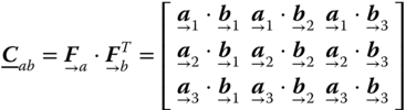
From 1.1 we have
where

The short expression then becomes
Switching the letters ![]() and
and ![]() ,
,
Orthonormality
It can be shown that matrices ![]() and
and ![]() are orthonormal when both frames of reference
are orthonormal when both frames of reference ![]() and
and ![]() are orthonormal; in other words they have orthonormal basis vectors.
are orthonormal; in other words they have orthonormal basis vectors.
Principal Rotations
There are three principal (basic) rotations of our interest:
-
 about
about
 or
or
 (1.10)where
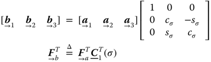
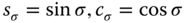 .
. -
 about
about
 or
or
 (1.11)
-
 about
about
 or
or
 (1.12)
1.2.2 The Motion of a Vector
The motion of a vector represents its rate of change with time, which is described as the time derivative of the vector. Consider a vector ![]() and its expressions
and its expressions ![]() and
and ![]() with respect to the reference frame
with respect to the reference frame ![]() and
and ![]() respectively; that is,
respectively; that is,
The time derivative is a vector itself, and also has different expressions under these two frames of reference:

Obviously, the expression of time derivative vector ![]() depends on the time derivative of the vectrix, or the change of rate of basis vectors of the associated frame of reference.
depends on the time derivative of the vectrix, or the change of rate of basis vectors of the associated frame of reference.
Absolute and Relative Time Derivatives
Assume ![]() represents an inertial space (a Newtonian absolute space). To an observer in
represents an inertial space (a Newtonian absolute space). To an observer in ![]() , the basis vectors of
, the basis vectors of ![]() , or the vectrix
, or the vectrix ![]() , will remain unchanged (no orientation change, and no magnitude change of course, since they are unit vectors). In other words, the first term in 15 is zero. Since
, will remain unchanged (no orientation change, and no magnitude change of course, since they are unit vectors). In other words, the first term in 15 is zero. Since ![]() is an inertial frame, we define the time derivative of a vector
is an inertial frame, we define the time derivative of a vector ![]() in
in ![]() as an absolute time derivative, denoted by a bullet
as an absolute time derivative, denoted by a bullet ![]() superscript:
superscript:
Assume ![]() is a moving frame of reference relative to
is a moving frame of reference relative to ![]() . Denote the moving (rotating) rate of change with time by
. Denote the moving (rotating) rate of change with time by ![]() . Similarly, to an observer in
. Similarly, to an observer in ![]() , the vectrix
, the vectrix ![]() also remains unchanged. In other words, the first term in 16 is zero. Therefore, the time derivative of a vector
also remains unchanged. In other words, the first term in 16 is zero. Therefore, the time derivative of a vector ![]() in the moving frame
in the moving frame ![]() is defined as a relative time derivative, denoted by a circle
is defined as a relative time derivative, denoted by a circle ![]() superscript:
superscript:
We here note that ![]() and
and ![]() are two different vectors,
are two different vectors,
However, they are closely related to each other.
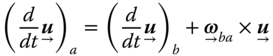
The definitions of absolute and relative derivatives are special cases of the following general expressions for time derivatives in a frame of reference. To an observer in a frame of reference ![]() (
(![]() ) the basis vectors of the frame, or the vectrix, remain unchanged. Hence,
) the basis vectors of the frame, or the vectrix, remain unchanged. Hence,
and the special cases are:
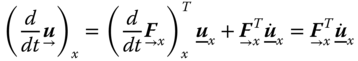
The time derivative of a vector ![]() in the frame of reference
in the frame of reference ![]() becomes:
becomes:
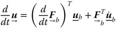
However, when dealing with multiple frames of reference in one frame ![]() , the basis vector of another frame
, the basis vector of another frame ![]() is no longer unchanged with time. Therefore, it leads to
is no longer unchanged with time. Therefore, it leads to
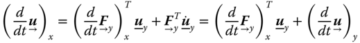
In other words, the motion of a vector in frame ![]() consists of the motion of this vector in frame
consists of the motion of this vector in frame ![]() and the motion of frame
and the motion of frame ![]() relative to frame
relative to frame ![]() .
.
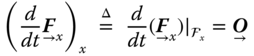
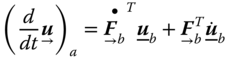
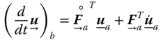
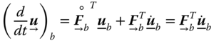
Returning to our previous special cases (absolute and relative derivatives), 15 and 16:
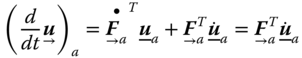
For the absolute derivative ![]() , we often drop the subscript
, we often drop the subscript ![]() .
.
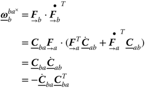
The focus now is placed on the rate of change of frame ![]() relative to another frame
relative to another frame ![]() .
.
Relative Rotation
To begin with, we look at the rotation of ![]() relative to
relative to ![]() about a fixed axis
about a fixed axis ![]() ,
,
One can conclude that, for a unit vector ![]() such as the axes of
such as the axes of ![]() ,
,
where the symbol ![]() between two vectors denotes the the cross product or vector product in three‐dimensional space (see Section 4.5.3 in the book by Polyanin and Manzhirov [1] for a definition).
between two vectors denotes the the cross product or vector product in three‐dimensional space (see Section 4.5.3 in the book by Polyanin and Manzhirov [1] for a definition).
General Rotation
Generally speaking, the angular velocity not only changes with the magnitude ![]() , but also changes its rotational orientation (there is no fixed axis). In other words, we are looking for a general description for angular velocity (general angular velocity), one that it is not associated with
, but also changes its rotational orientation (there is no fixed axis). In other words, we are looking for a general description for angular velocity (general angular velocity), one that it is not associated with ![]() like the one we had before: we are dealing with the general rotation case. From the previous case, we would like to see a general description of angular velocity, such that for an unit vector
like the one we had before: we are dealing with the general rotation case. From the previous case, we would like to see a general description of angular velocity, such that for an unit vector ![]() , the following equation still holds:
, the following equation still holds:
On the one hand,

and on the other hand,
Therefore,
Consider the arbitrary unit vector ![]() . We must have
. We must have
We define general angular velocity as:
where the expression matrix ![]() is given by
is given by
By that definition, we have the conclusion of an expression for general rotation 31.
To conclude, for the general rotation of a basis vector, we have

Matrix Expression
From definition 1.37 and relationship equation 1.4, we have
From a different perspective, for a unit vector ![]()

On the other hand,
Therefore, ![]()
In summary,
1.2.3 The First Time Derivative of a Vector
Consider the time derivative of an arbitrary vector,
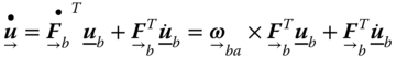
Since
we have:
Furthermore,

In summary
Pure Translation
We say ![]() is in pure translation with respect to
is in pure translation with respect to ![]() if the rotation matrix
if the rotation matrix ![]() is constant in time; in other words, if the orientation of the basis vectors of one frame relative to the basis vectors of the other frame remains fixed. In other words, there might be rotation from
is constant in time; in other words, if the orientation of the basis vectors of one frame relative to the basis vectors of the other frame remains fixed. In other words, there might be rotation from ![]() to
to ![]() , but there is no change of that rotation in time. Then,
, but there is no change of that rotation in time. Then,
leading to
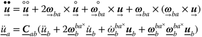
1.2.4 The Second Time Derivative of a Vector
We can treat the second derivative as the first derivative of vector ![]() ,
,

In summary
Another observation is:
1.2.5 Motion with Respect to Multiple Frames
Here, we will formally prove that
Time Derivatives
Assume a fixed (inertial, absolute) frame of reference ![]() and two moving frames of reference
and two moving frames of reference ![]() and
and ![]() , each rotating relative to
, each rotating relative to ![]() at rates of
at rates of ![]() and
and ![]() respectively. Then we have
respectively. Then we have

If we denote the absolute derivative by ![]() , the relative derivative in
, the relative derivative in ![]() by
by ![]() , and the relative derivative in
, and the relative derivative in ![]() by
by ![]() , then the above equations become
, then the above equations become

Note that the absolute time derivative formulae looks the same as each other, but the rotating rates are different.
1.3 Euler Parameters and Unit Quaternion
Euler's theorem states that any rotation of an object in 3‐D space leaves some axis fixed: this is the rotation axis. As a result, any rotation can be described by a unit vector ![]() (satisfying
(satisfying ![]() ) in the direction of the rotational axis, and the angle of rotation,
) in the direction of the rotational axis, and the angle of rotation, ![]() , about
, about ![]() . The rotation matrix is represented by
. The rotation matrix is represented by
where the set ![]() is often called the Euler axis/angle variables.
is often called the Euler axis/angle variables.
To avoid a triangular calculation, these variables can be replaced by the so‐called Euler parameters:
Note that ![]() . Then the rotation matrix becomes
. Then the rotation matrix becomes
Now, let us take a look at the rotation matrix corresponding to two consecutive rotations, represented by either their Euler axis/angle variables, or the Euler parameters,
After some tedious matrix algebraic manipulation, this leads to the following relationship:
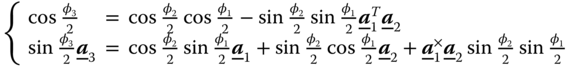
or

In matrix format, we obtain the following

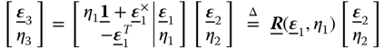
The matrix representation of ![]() is one of the expressions of the so‐called unit quaternion, denoted by
is one of the expressions of the so‐called unit quaternion, denoted by

In the current case,

It is obvious that ![]() . Therefore the Euler parameter is considered as a unit quaternion.
. Therefore the Euler parameter is considered as a unit quaternion.
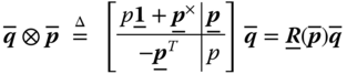
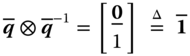
We define the quaternion multiplication as

Its inverse (representing a reverse rotation of angle ![]() about unit axis
about unit axis ![]() ) is defined by
) is defined by

and one can prove that
Using these definitions, we can obtain the formulation of attitude error. Assume ![]() and
and ![]() represent the desired attitude and actual attitude, respectively. The error between the actual and the desired attitudes can be treated as a consecutive rotation from the desired attitude,
represent the desired attitude and actual attitude, respectively. The error between the actual and the desired attitudes can be treated as a consecutive rotation from the desired attitude,
This leads to
In other words,

This expression shows that the error attitude (quaternion) is now represented by the actual attitude and the desired attitude. Further, as ![]() , the steady error attitude
, the steady error attitude ![]() .
.
Under the Euler parameters or unit quaternion, the angular rate vector ![]() is described as
is described as
and
