4
Output‐feedback Solutions to Formation Control
4.1 Introduction
For an angular‐position synchronization control problem or a formation control problem, we may view the (linear or angular) position signals as the output of the considered MVS. In this chapter, we introduce a comprehensive treatment of angular‐position synchronization control and formation control without velocity signals. These control problems are two typical output feedback control problems associated with MVSs.
4.2 Problem Statement
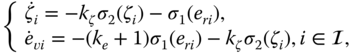
Recall the following MVS model:
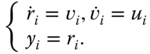
where ![]() denotes the linear (or angular) position of vehicle
denotes the linear (or angular) position of vehicle ![]() and serves as the output of the
and serves as the output of the ![]() th vehicle system,
th vehicle system, ![]() is the corresponding linear (or angular) velocity, and
is the corresponding linear (or angular) velocity, and ![]() is the control input. For simplicity, we here assume that the dimensions of all the involved variables is 1.
is the control input. For simplicity, we here assume that the dimensions of all the involved variables is 1.
In this section, we mainly introduce the design of synchronization control for MVSs ((4.1)) under the constraint that only position signals ![]() ,
, ![]() are accessible for control design. In other words, the velocity signals
are accessible for control design. In other words, the velocity signals ![]() ,
, ![]() ,
, ![]() are not accessible for control design. This control problem can be regarded as an output‐feedback control problem of a higher‐order (
are not accessible for control design. This control problem can be regarded as an output‐feedback control problem of a higher‐order (![]() th‐order) linear system. Since the MVS is completely observable, an intuitive idea to deal with this problem is based on the well‐known Luenberger state observer (LSO) theory for observable linear systems [1]. The application of this theory generally consists of two steps:
th‐order) linear system. Since the MVS is completely observable, an intuitive idea to deal with this problem is based on the well‐known Luenberger state observer (LSO) theory for observable linear systems [1]. The application of this theory generally consists of two steps:
- Design a full‐order state observer for each vehicle to obtain an asymptotic estimate of the actual state.
- Replace the actual state variables of vehicles used in state‐feedback controllers with their estimates (the estimates of neighboring vehicles' states are also often needed).
The separation principle ensures that this LSO‐based approach works well for a linear system. A detailed design is omitted here for simplicity, and the readers are referred to the literature for design examples [2]. Instead, we will detail here the application of an alternative approach, called the passivity approach, which is based on the design of a simple first‐order linear filter. We will further show that by introducing this filter into the system, the asymptotic estimates of vehicle velocities are not required. Similar applications of such an approach can be found in Section 4.3 of the book by Ren and Beard [3] and the paper by Lawton et al. [4].
4.3 Linear Output‐feedback Control
The control strategy (3.85) for synchronized position tracking requires that the relative velocities between neighbors, and/or the velocity tracking error, are known. However, in the context of this chapter, neither the relative velocity or the velocity tracking error is accessible for control design. To resolve a similar issue, Lawton et al. developed a decentralized approach using a passivity technique to inject relative damping into the system, where the relative damping is produced by a first‐order linear filter [4].
Motivated by their approach, and using the Type III LSEs, ![]() , defined by (3.48), we construct the following dynamic output‐feedback control law for system 1:
, defined by (3.48), we construct the following dynamic output‐feedback control law for system 1:

where ![]() , with an arbitrary initial value
, with an arbitrary initial value ![]() , is the state of the introduced first‐order auxiliary equation included in (4.2), and
, is the state of the introduced first‐order auxiliary equation included in (4.2), and ![]() and
and ![]() are strictly positive control gains.
are strictly positive control gains.
It is seen from (4.2) that the desired acceleration signal ![]() is required to be accessible to each vehicle. However, when the desired velocity,
is required to be accessible to each vehicle. However, when the desired velocity, ![]() , is a constant,
, is a constant, ![]() and the requirement is naturally removed.
and the requirement is naturally removed.
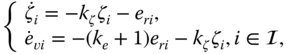
Combining (4.1) and (4.2), yields the closed‐loop system
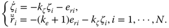
The two equations included in (4.3) are mutually coupled, because ![]() appears in the first equation and
appears in the first equation and ![]() in the second. Moreover, the state variables used in the two sides of (4.3) are not identical. Specifically, the left‐hand side adopts variable
in the second. Moreover, the state variables used in the two sides of (4.3) are not identical. Specifically, the left‐hand side adopts variable ![]() , while the right‐hand side adopts variable
, while the right‐hand side adopts variable ![]() . For these reasons, it is not realistic to analyse the stability of the node‐level system with the Routh criterion or matrix theory. Applying the linear system approaches to network‐level closed‐loop dynamics is not easy either, because the system order,
. For these reasons, it is not realistic to analyse the stability of the node‐level system with the Routh criterion or matrix theory. Applying the linear system approaches to network‐level closed‐loop dynamics is not easy either, because the system order, ![]() , is high and not known (the number of vehicles involved,
, is high and not known (the number of vehicles involved, ![]() , is not fixed in advance).
, is not fixed in advance).
Therefore, we here do not dwell on the application of linear system approaches to MVSs (4.3). Instead, we apply the Lyapunov function approach and LaSalle's invariance principle to obtain the following result.
4.4 Bounded Output‐feedback Control
Note that the ![]() defined by (3.48) are linear functions of
defined by (3.48) are linear functions of ![]() and
and ![]() . The values of
. The values of ![]() therefore depend linearly on those of
therefore depend linearly on those of ![]() and
and ![]() . Since the controller (4.2) is a linear function of
. Since the controller (4.2) is a linear function of ![]() , it suffers from the limitation that larger
, it suffers from the limitation that larger ![]() or
or ![]() may lead to actuator saturation. An intuitive and useful idea to avoid actuator saturation is to feed back saturated signals. In this section, we apply this idea to construct a bounded output‐feedback synchronized tracking controller.
may lead to actuator saturation. An intuitive and useful idea to avoid actuator saturation is to feed back saturated signals. In this section, we apply this idea to construct a bounded output‐feedback synchronized tracking controller.
We use the hyperbolic tangent function ![]() to modify the Type III LSEs as follows:
to modify the Type III LSEs as follows:

Note that, in order to ensure that the ![]() defined by (4.16) are bounded, we limit the bounds of components
defined by (4.16) are bounded, we limit the bounds of components ![]() and
and ![]() . This is different from the traditional applications of saturation functions, where the signal is not bounded component‐wise (see Lemma A.15 in Appendix A.2.5 for the definition and properties of generalized saturation functions). We also note that, as for a higher‐dimensional motion, the hyperbolic tangent function
. This is different from the traditional applications of saturation functions, where the signal is not bounded component‐wise (see Lemma A.15 in Appendix A.2.5 for the definition and properties of generalized saturation functions). We also note that, as for a higher‐dimensional motion, the hyperbolic tangent function ![]() in (4.16) is defined element‐wise for vectors
in (4.16) is defined element‐wise for vectors ![]() and
and ![]() .
.
To make a difference, we refer to the ![]() defined by (4.2) and (4.16) as the linear and nonlinear LSEs, respectively. As shown in Lemma 3.3, under Condition 3, the convergence of linear
defined by (4.2) and (4.16) as the linear and nonlinear LSEs, respectively. As shown in Lemma 3.3, under Condition 3, the convergence of linear ![]() (
(![]() ) is sufficient and necessary to ensure the convergence of tracking errors
) is sufficient and necessary to ensure the convergence of tracking errors ![]() (
(![]() ). To render the design and analysis clear, we expect that this property remains for the nonlinear LSEs. Clearly, if
). To render the design and analysis clear, we expect that this property remains for the nonlinear LSEs. Clearly, if ![]() tends to zero for each
tends to zero for each ![]() , so will the components
, so will the components ![]() and
and ![]() . Then, the remaining question is whether we can derive the convergence of
. Then, the remaining question is whether we can derive the convergence of ![]() from the convergence of
from the convergence of ![]() defined by (4.16). The following provides a clear answer to that question.
defined by (4.16). The following provides a clear answer to that question.
In light of the results of Lemma 4.2, the problem of stabilizing ![]() ,
, ![]() , under Condition 4 can be solved by stabilizing
, under Condition 4 can be solved by stabilizing ![]() ,
, ![]() . Therefore, the remaining task is to design
. Therefore, the remaining task is to design ![]() to render
to render ![]() ,
, ![]() .
.
Using ![]() defined in (4.16), we construct the following control law:
defined in (4.16), we construct the following control law:

where ![]() , with an arbitrary initial value
, with an arbitrary initial value ![]() , is the state of the introduced nonlinear auxiliary system, and
, is the state of the introduced nonlinear auxiliary system, and ![]() is a strictly positive gain.
is a strictly positive gain.
From (4.16) and (4.23), we readily derive that
This indicates that ![]() determined by (4.23) are indeed prior bounded.
determined by (4.23) are indeed prior bounded.
The closed‐loop dynamics consisting of (4.1) and (4.23) are described by

for which we have the following result.
As for MVS (4.25), it is important to note the following two facts:
- System (4.25) is autonomous, implying that the LaSalle invariance theorem in typical form [7] is applicable.
- The symmetry property of an undirected graph– that is,
 ,
,  – is used in the proof of Theorem 4.3. This indicates that the result of the theorem cannot be directly extended to the case with a directed subgraph
  , despite the fact that the full rank condition on
  or
or  does not necessarily require subgraph
  to be undirected.
4.5 Distributed Linear Control
To implement the control law (4.2), the desired acceleration signal ![]() is required for each vehicle in the MVS. This is rather restrictive. To remove this limitation, we consider the following control law:
is required for each vehicle in the MVS. This is rather restrictive. To remove this limitation, we consider the following control law:

where ![]() ,
, ![]() , are linear Type III LSEs, and
, are linear Type III LSEs, and ![]() and
and ![]() are positive control gains defined as in (4.2).
are positive control gains defined as in (4.2).
The differences between the control laws (4.2) and (4.27) are two‐fold.
- The term
 in (4.2) is replaced by
  in (4.27).
 - All four components of
 in (4.27) share a common coefficient
  , whose value depends on the information‐exchange weights associated with node
  (see Equation (3.63)). However, this is not the case for
  in (4.2).
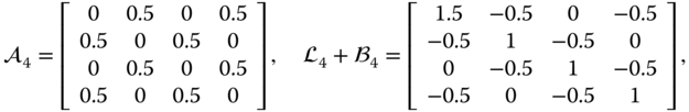
The closed‐loop dynamics consisting of (4.1) and (4.27) are
which can be written in a vector form as
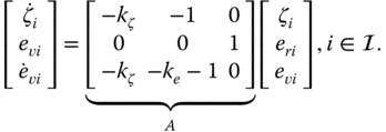
A simple calculation shows that the characteristic polynomial of system matrix ![]() is
is
It is easy to check that the polynomial is Hurwitz provided ![]() and
and ![]() . Thus we have the following result.
. Thus we have the following result.
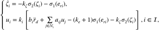
4.6 Distributed Bounded Control
The controller (4.27) is linear and not prior bounded. Suppose ![]() and
and ![]() are two generalized saturation functions (GSFs), as defined in Lemma A.15 in Appendix A.2. To obtain a bounded controller, we modify (4.27) using GSFs as
are two generalized saturation functions (GSFs), as defined in Lemma A.15 in Appendix A.2. To obtain a bounded controller, we modify (4.27) using GSFs as
where ![]() and
and ![]() are saturation functions defined element‐wise for a vector argument, and
are saturation functions defined element‐wise for a vector argument, and ![]() satisfies the additional condition
satisfies the additional condition
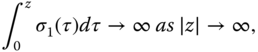
which is trivially satisfied if ![]() . This condition ensures that the Lyapunov function candidate considered in the proof of Theorem 4.5 (i.e., Equation 4.35) is radially unbounded.
. This condition ensures that the Lyapunov function candidate considered in the proof of Theorem 4.5 (i.e., Equation 4.35) is radially unbounded.
The closed‐loop system consisting of (4.1) and (4.31) is described by
where the gains ![]() and
and ![]() are defined as in (4.27).
are defined as in (4.27).
We then have the following result.
4.7 Simulations
In this section, we verify the theoretical results from the previous sections by simulation. In particular, we present the simulation results of two cases which correspond to the linear control considered in Theorem 4.1 and the prior bounded control considered in Theorem 4.5, respectively. In each case, four followers and a virtual leader are involved, and the motion is planar two‐dimensional (i.e., ![]() ,
, ![]() and
and ![]() in (4.1)).
in (4.1)).
4.7.1 Case 1: Verification of Theorem 4.1
Consider the interaction graph shown in Figure 3.2d (or Figure 4.1), which trivially satisfies Condition 4 with an undirected and connected ![]() and node 1 having access to the leader. For control law (4.2), we here suppose
and node 1 having access to the leader. For control law (4.2), we here suppose
which implies ![]() and
and ![]() . The gains for each dimension of each vehicle are the same, with
. The gains for each dimension of each vehicle are the same, with ![]() .
.
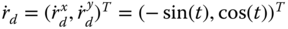
The desired trajectories are:
-
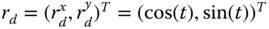
-
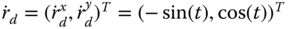
-
 .
.
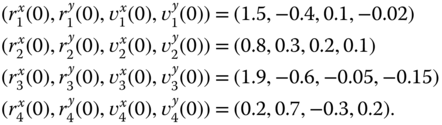
The initial states of the four vehicles are:

The initial states of the auxiliary system involved in (4.2) are: ![]() ,
, ![]() . The Matlab R2014a/simulation solver ode3 (Bogacki‐Shampine) with a fixed‐step size of 0.01 s is used in the simulation.
. The Matlab R2014a/simulation solver ode3 (Bogacki‐Shampine) with a fixed‐step size of 0.01 s is used in the simulation.
The simulation results are presented in Figures 4.2–4. As shown in Figures 4.2 and 3, the position trajectories of each vehicle converge asymptotically to the desired trajectories, and the settling time is about 28 s to ensure the bounds of tracking errors and synchronization errors are smaller than 0.05. Figure 4.4 shows that the actual trajectory of each vehicle tracks asymptotically the desired 2‐D circular trajectory (with radius 1).
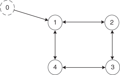
Figure 4.1 The interaction graph for Case 1.

Figure 4.2
The  ‐axis position trajectories for Case 1.
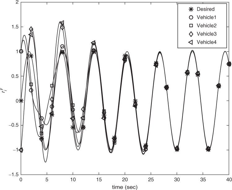
Figure 4.3
The  ‐axis position trajectories for Case 1.

Figure 4.4 The planar position trajectories vs. time for Case 1.
4.7.2 Case 2: Verification of Theorem 4.5
The interaction graph is shown in Figure 4.5. It trivially satisfies Condition 3 with node 0 (the leader) as the root node and a directed subgraph ![]() describing the interaction among the four vehicles. To be specific, for the bonded controller (4.31) we set
describing the interaction among the four vehicles. To be specific, for the bonded controller (4.31) we set
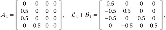
which implies ![]() and
and ![]() . The saturation functions
. The saturation functions ![]() are used, and the gains for each dimension of each vehicle are the same, with
are used, and the gains for each dimension of each vehicle are the same, with ![]() . The desired trajectories are:
. The desired trajectories are:
-

-
-
 .
.
The initial states of the four vehicles are:
The initial values of ![]() (
(![]() ) are zero in
) are zero in ![]() . Matlab R2014a/simulation solver ode3 (Bogacki‐Shampine) with a fixed‐step size of 0.01 s is used in the simulation.
. Matlab R2014a/simulation solver ode3 (Bogacki‐Shampine) with a fixed‐step size of 0.01 s is used in the simulation.
The simulation results are presented in Figures 4.6–4.8. As shown in Figures 4.6 and 4.7, the position trajectories of each vehicle converge asymptotically to the desired trajectories and the settling time is about 13 s for bounds of tracking errors and synchronization errors smaller than 0.05. Figure 4.8 further shows that the actual planar motion trajectory of each vehicle tracks asymptotically the desired 2‐D circular trajectory (with radius 1).

Figure 4.5 The interaction graph for Case 2.
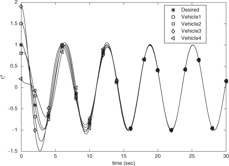
Figure 4.6
The  ‐axis position trajectories for Case 2.

Figure 4.7
The  ‐axis position trajectories for Case 2.
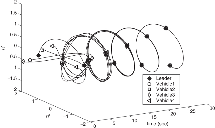
Figure 4.8 The planar position trajectories vs. time for Case 2.
4.8 Summary
Note that all the controllers discussed in Chapter 3 use full state feedback: both position and velocity signals are used in the controller design. In contrast, this chapter discusses the controller design without velocity measurements. In particular, four different output‐feedback control laws for synchronized position trajectory tracking are developed using passivity techniques. Once a formation control problem is converted to a synchronized tracking problem (as shown in Chapter 3), all the control laws can be easily applied to achieve formation motion.
These control laws are given in (4.2), (4.23), (4.27) and (4.31), respectively. We also recall that the two control laws given in (4.23) and (4.31), respectively, are non‐linear, each of which accounts for the actuator saturation constraint. The non‐linear control laws are important in practice since actuator saturation may lead to actuator chattering, or even loss of system stability. Compared with the closed‐loop MVS dynamics resulting from the two linear control laws, the closed‐loop dynamics resulting from the two non‐linear control laws are more complicated. Despite this, the two non‐linear control laws ensure that the synchronized tracking objective is asymptotically achieved by prior bounded control.
It is important to note that all the four control laws share the following two common features:
- The signals
 ,
,  and
and  for
for  , are not used for control design.
 - The dimension of the controlled motion described by (4.1) is not limited to a certain number. Therefore, these control laws may be applicable to synchronized tracking in either 1‐dimensional, 2‐dimensional, or 3‐dimensional space.
In the next chapter, we will systematically investigate control design for robustness improvement with respect to input disturbances, which is another issue of practical importance, and is associated with synchronized tracking as well as formation control.