9
Experiments on 3DOF Desktop Helicopters
In this chapter, we will first introduce an experimental apparatus, which consists of four Quanser Inc.'s desktop “helicopters”, and then show how the control concepts and approaches introduced in Chapter 6 are applied to this experimental apparatus. In particular, we will present several laboratory cases and show the experimental results obtained.
9.1 Description of the Experimental Setup
As a case study to illustrate the main control concepts and results presented in this book, an experimental apparatus is set up as a possible laboratory exercise. The so‐called desktop three‐degree‐of‐freedom “helicopters” (3DOF‐Heli) used are shown in Figure 9.1: as can be seen, they are a desktop model of a helicopter rather than a helicopter per se. Four of them serve as a platform for conducting experiments on multiple vehicles.
Before the details of the experimental setup are introduced, one may wonder how representative this laboratory equipment can be. How realistic are they in terms of reflecting real‐world applications? Of course, they are not commercial systems, yet, one may find in the 3DOF‐Heli some resemblances to real‐world applications. It is not difficult to understand where the “helicopter” name comes from when one sees a 3DOF‐Heli “fly” like a real two‐rotor helicopter (which is also called as a tandem rotor helicopter, with one rotor in the front and the other at the back of the vehicle) such as:
- the Piasecki HRP Rescuer, designed by Frank Piasecki and built by Piasecki Helicopter;
- the Boeing CH‐47 Chinook, an American twin‐engine, tandem rotor heavy‐lift helicopter, the primary roles of which are troop movements, artillery placement and battlefield resupply;
- the Boeing Model 360, an experimental medium‐lift tandem rotor cargo helicopter developed privately by Boeing to demonstrate advanced helicopter technology.
In addition, the 3DOF‐Heli's lifting device, driven by DC motors, provides an excellent representation of the second‐order systems that are often found in space, aerial and robotics applications. The DC motor offers plenty of opportunities to address the nonlinearities, uncertainties or measurement errors involved.
The apparatus is well designed, easy to operate, and there are many examples of experiments and simulations that the reader can find in the literature to enrich their study. The 3DOF‐Heli equipment is supplied by Quanser Consulting Inc.,a well regarded company in the control engineering education community.
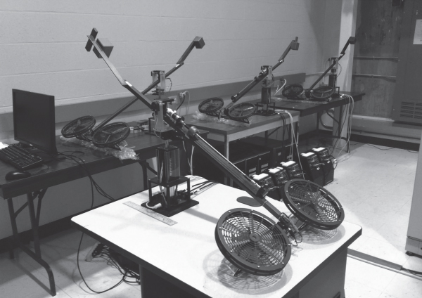
Figure 9.1 The setup of four 3DOF‐Helis.
There are four 3DOF‐Helis at the Flight Systems and Control (FSC) Laboratory of the University of Toronto. They are used for studying cooperative control of MVSs, multivehicle formation flight control, and advanced controller development. The comprehensive experimental configuration and signal flow chart is shown in Figure 9.2, where all four helicopters are involved. Experimental configurations with fewer helicopters are easily obtained.
As shown in Figure 9.2, four helicopters (H1 to H4), ten universal power modules (UPMs), two Q8 terminal boards and a PC are included in this configuration. Helicopters H2 and H4 are equipped with active disturbance systems (ADSs), whereas the H1 and H3 are not. The elevation and pitch angles and the position signals of the ADSs are measured using encoders installed on the helicopters and transmitted through the Q8 terminal boards to two Q8 data acquisition cards (DACs), which are installed on the PC. The resolution of each encoder is 4096 counts per revolution, which yields a resolution of ![]() for the angular position measurement. For H1 (or H3), two UPMs are used to supply power to the front and back DC motors (propellers), respectively. For H2 (or H4), an additional UPM is used for the ADS motor. One of the two Q8 terminal boards is used for H1 and H2, and the other is for H3 and H4. Each terminal board is connected to one Q8 DAC. In each experiment, the sampling time is fixed to be 0.001 s, and the implemented control laws are constructed using Simulink blocks, compiled and downloaded to Q8 DACs and run in real‐time therein. The real‐time experimental data from the Q8 DAC are sent to a PC through a PCI computer bus. For the full‐state feedback, the elevation and pitch angular rates are generated using second‐order derivative filters provided by Quanser Consulting Inc. 1.
for the angular position measurement. For H1 (or H3), two UPMs are used to supply power to the front and back DC motors (propellers), respectively. For H2 (or H4), an additional UPM is used for the ADS motor. One of the two Q8 terminal boards is used for H1 and H2, and the other is for H3 and H4. Each terminal board is connected to one Q8 DAC. In each experiment, the sampling time is fixed to be 0.001 s, and the implemented control laws are constructed using Simulink blocks, compiled and downloaded to Q8 DACs and run in real‐time therein. The real‐time experimental data from the Q8 DAC are sent to a PC through a PCI computer bus. For the full‐state feedback, the elevation and pitch angular rates are generated using second‐order derivative filters provided by Quanser Consulting Inc. 1.
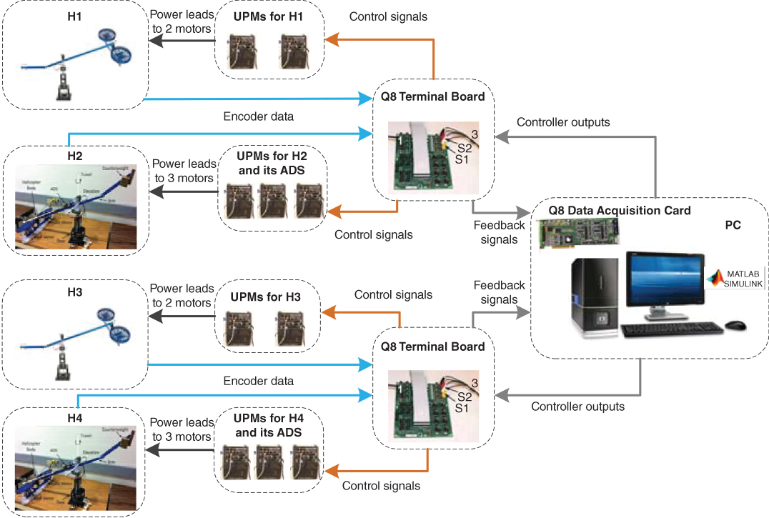
Figure 9.2 The hardware configuration of the experimental setup.
9.2 Mathematical Models
9.2.1 Nonlinear 3DOF Model
To obtain the nonlinear 3‐DOF motion model of a helicopter, we first introduce its hardware components. Photos of a single helicopter are shown in Figures 9.3–9.5. Two DC motors are used to drive the propellers, which in turn generate control forces to regulate the 3‐DOF motions of the helicopter. These motors are defined as the front and the back motors respectively. The body frame is suspended from an instrumented joint, which connects the centre of the body frame and the end of a long arm, and is free to pitch about its centre. The arm is installed on the base through a 2‐DOF instrumented joint, which allows the helicopter body to elevate and travel. A counterweight is located at the other end of the arm such that the effective mass of the helicopter can be adjusted to a suitable value. In addition, an optional ADS can be installed on the arm. This includes an ADS motor that can drive an adjustable weight moving along the arm. The ADS motor is controlled independently, and therefore can act as an external disturbance or model uncertainty. The elevation motion can be generated by applying a positive voltage to each motor, and positive pitch by applying greater voltage to the front motor. The travel motion is the result of tilted thrust vectors when the body pitches. The three attitude angles are measured by encoders mounted on the instrumented joints. Therefore, pitch, elevation, and travel are the three degrees of freedom from which the 3DOF‐Heli gets its name.

Figure 9.3 The 3DOF‐Heli components.
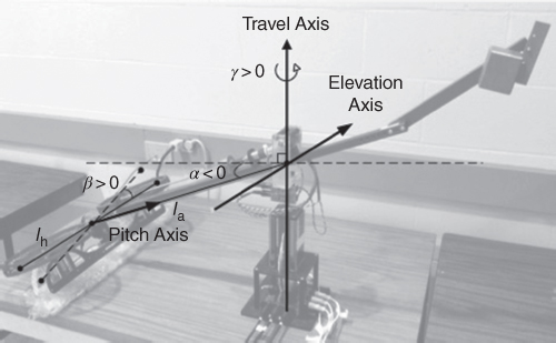
Figure 9.4 3DOF‐Heli body frame.

Figure 9.5 Hardware configuration of 3DOF‐Heli body.
A convenient way to describe the motions of the 3DOF‐Heli is through a body‐frame defined along the axes of the equipment, centralized around the baseline rotational pivot, as shown in Figure 9.4. For a fleet of ![]() 3DOF‐Helis, the nomenclature associated with the
3DOF‐Helis, the nomenclature associated with the ![]() th 3DOF‐Heli,
th 3DOF‐Heli, ![]() , is as follows:
, is as follows:
-
 is the elevation angle;
 -
 is the elevation rate;
 -
 is the pitch angle;
 -
 is the pitch rate;
 -
 is the travel angle;
 -
 is the travel rate;
 -
 ,
,  , and
, and  are the moments of inertia about the elevation axis, pitch axis, and travel axis, respectively;
 -
 is the force constant of the motor–propeller combination;
 -
 is the distance from the elevation axis to the centre of the helicopter body;
 -
 is the distance from the pitch axis to either motor;
 -
 is the effective mass of the helicopter body;
 -
 is the gravitational acceleration constant;
 -
 ,
,  , and
, and  denote disturbances acting on the elevation channel, pitch channel and travel axis, respectively;
 -
 and
and  are the voltages applied to the front motor and back motor, respectively;
 -
 and
and  denote the sum and the difference of
  and
and  , respectively.
The differential equation of motion for the ![]() the laboratory experimental setup, which can be derived using the Lagranges formalism, is written in the following well‐known form (see examples in the literature [2, 3] and Chapter 6):
the laboratory experimental setup, which can be derived using the Lagranges formalism, is written in the following well‐known form (see examples in the literature [2, 3] and Chapter 6):
where the inertia matrix ![]() , the Coriolis matrix
, the Coriolis matrix ![]() , the gravity vector
, the gravity vector ![]() , the disturbance input
, the disturbance input ![]() , the generalized forces
, the generalized forces ![]() , and the state variable vector
, and the state variable vector ![]() .
.
For simplicity, the generalized inertia matrix ![]() is often reduced to a diagonal matrix with constant entries. To be specific, the mathematical model of the form (1) for the
is often reduced to a diagonal matrix with constant entries. To be specific, the mathematical model of the form (1) for the ![]() th 3DOF‐Heli reads as follows:
th 3DOF‐Heli reads as follows:
where
and:
-
Equation
(9.2)
describes the elevation dynamics: Due to the presence of the counterweight, the second‐order equation of motion accounts for the pendulum‐like oscillatory characteristic, where
 is the vertical lift thrust component,
  is the restorative spring torque,
  is the torque generated because the pivot points of the elevation and pitch motions are not exactly in the helicopter's body, and
  is the unknown aerodynamic and mechanical damping torque.
 -
Equation
(9.3)
describes the pitch dynamics: Here, the second‐order equation of motion accounts for the lightly‐damped oscillatory characteristics:
 is the rotor torque,
  the restorative spring torque, and
  is the rotor damping.
 -
Equation
(9.4)
describes the travel dynamics: Here,
 is the propulsive thrust component resulting from the pitch motion with a nonzero
  ;
;  is the unknown aerodynamic drag as well as some amount of mechanical friction at the hinge.
Consider the equations of motion given in (9.10)–(9.12) with relationship equations (9.6). The electric voltage ![]() controls collectively the speed of the two propellers, and a positive
controls collectively the speed of the two propellers, and a positive ![]() produces a positive lifting moment. The electric voltage
produces a positive lifting moment. The electric voltage ![]() results in differential changes in the two rotor speeds, and a positive
results in differential changes in the two rotor speeds, and a positive ![]() produces a positive pitch moment.
produces a positive pitch moment.
Let
Then Equations (9.2)–(9.4) are reduced to:
In Equations (9.10)–(9.12), the aerodynamic drag, the mechanical friction, and the rotor damping are not explicitly considered. Instead, we take into account both model uncertainties and friction effects, by lumping them together as the additive input disturbances ![]() ,
, ![]() , and
, and ![]() .
.
9.2.2 2DOF Model for Elevation and Pitch Control
Assuming travel motion can be achieved by highly precise pitch tracking, we simplify the 3‐DOF attitude dynamics to 2‐DOFs, namely elevation and pitch. The simplified model describing the elevation and pitch motions of the ![]() th helicopter (
th helicopter (![]() ) is then:
) is then:
where the pitch angle, ![]() , is limited to the range
, is limited to the range ![]() mechanically, and the nominal values of the involved parameters are as presented in Table 9.1.
mechanically, and the nominal values of the involved parameters are as presented in Table 9.1.
Table 9.1
Nominal parameters of the helicopters (![]() ).
).
| Parameter | Value | Parameter | Value |
|
|
0.1188 N/V |
|
1.034 kg |
|
|
0.660 m |
|
0.045 kg |
|
|
0.178 m |
|
9.81 m/ |
|
|
0.094 kg |
Equations (9.13)–(9.14) can be written in the following compact form:
where

Since pitch angle ![]() is mechanically limited to the range
is mechanically limited to the range ![]() in all experiments, the inertia matrix
in all experiments, the inertia matrix ![]() for each
for each ![]() is a positive‐definite matrix.
is a positive‐definite matrix.
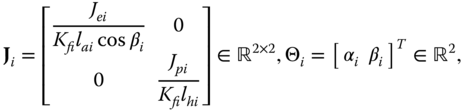
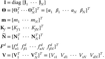
Equation (9.15) can be formulated in matrix format as:
where ![]() ,
, ![]() ,
, ![]() ,
, ![]() ,
, ![]() , and
, and ![]() are vectors, and
are vectors, and ![]() is a diagonal inertia matrix. These vectors have the following expressions:
is a diagonal inertia matrix. These vectors have the following expressions:
Since ![]() ,
, ![]() , for any
, for any ![]() , Equation 9.19 is equivalent to:
, Equation 9.19 is equivalent to:
where
We use ![]() to denote the desired angular‐position trajectories for the four helicopters, and
to denote the desired angular‐position trajectories for the four helicopters, and ![]() the desired angular‐velocity trajectories. For
the desired angular‐velocity trajectories. For ![]() helicopters, 2‐D mutual angular‐position synchronization means that:
helicopters, 2‐D mutual angular‐position synchronization means that:
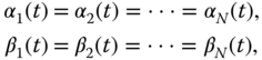
and 2‐D zero‐error trajectory tracking in angular position means

Correspondingly, the 2‐D mutual angular‐velocity synchronization means

and the 2‐D zero‐error trajectory tracking in angular velocity means
In the context of this application, synchronization error is used to identify how the attitude trajectories of each 3‐DOF helicopter converge with respect to each other.
Let:
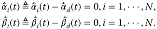
Then, MVS (9.15) can be modelled by the vector equation (5.4) or the following two decoupled scalar equations:
where ![]() with
with ![]() (
(![]() ) is the control input vector to be determined, and
) is the control input vector to be determined, and ![]() with
with ![]() (
(![]() ) is the normalized disturbance input vector. This further implies that the control concepts and approaches introduced in Chapter 6 are applicable in designing
) is the normalized disturbance input vector. This further implies that the control concepts and approaches introduced in Chapter 6 are applicable in designing ![]() for the MVS considered.
for the MVS considered.
Once ![]() or
or ![]() has been determined,
has been determined, ![]() are computed according to Equation (9.27). Therefore, in each of the experiments below, the design of
are computed according to Equation (9.27). Therefore, in each of the experiments below, the design of ![]() or
or ![]() is the main focus: we will introduce several control experiments where objectives (9.23)–(9.26) are achieved in an asymptotic manner or an approximately asymptotic manner. We start by introducing an experiment in which the GSE‐based synchronized tracking controller developed in Section is applied and implemented.
is the main focus: we will introduce several control experiments where objectives (9.23)–(9.26) are achieved in an asymptotic manner or an approximately asymptotic manner. We start by introducing an experiment in which the GSE‐based synchronized tracking controller developed in Section is applied and implemented.
9.3 Experiment 1: GSE‐based Synchronized Tracking
9.3.1 Objective
The experiments are conducted on a platform consisting of three 3‐DOF helicopters, which are labelled Heli. I, Heli. II and Heli. III, respectively, as shown in Figure 9.6. The model parameters for control design are given in Table 9.2.
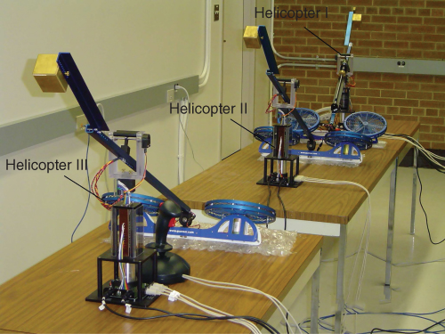
Figure 9.6 Experimental setup with three 3DOF‐Helis.
Table 9.2 Parameters and control gains.
| Parameter/gain | Heli. I | Heli. II | Heli. III |
|
|
1.044 | 1.030 | 1.017 |
|
|
0.0455 | 0.0455 | 0.0455 |
| Mass |
0.142 1 | 0.128 | 0.113 |
|
|
0.625 | 0.625 | 0.625 |
|
|
0.648 | 0.648 | 0.648 |
|
|
0.178 | 0.178 | 0.178 |
| ADS system | Yes | No | No |
| Feedback gains, [ |
[30.0 15.0] | [30.0 15.0] | [30.0 15.0] |
| Sync. feedback gains, |
1.0 | 1.0 | 1.0 |
| Sync. coupling gains, |
1.0 | 1.0 | 1.0 |
Value measured when ADS is at the farthest position from propellers, 0.170 for the middle position in the slide bar, 0.213 for the nearest position from propellers.
The objectives of this experiment are:
- to design a controller using the approach proposed in Section for the elevation axis, to achieve synchronized trajectory tracking asymptotically; that is, to achieve (9.23)–(9.26) asymptotically;
- to implement the controller and compare its performance to that of a controller without GSE feedback (obtained by setting
 and
and  ,
,  , in controller (5.142));
 - to verify the robustness of the proposed controller with respect to the disturbances resulting from activated ADSs.
9.3.2 Initial Conditions and Desired Trajectories
A quintic polynomial trajectory in (9.31) is designed for the attitude motion of the elevation:

where the coefficients ![]() can be determined from the position, velocity, and acceleration requirements at both boundaries. If the desired maneuver is from 0 to
can be determined from the position, velocity, and acceleration requirements at both boundaries. If the desired maneuver is from 0 to ![]() in 8 s, the coefficients are
in 8 s, the coefficients are ![]() ,
, ![]() ,
, ![]() and
and ![]() . This trajectory guarantees that
. This trajectory guarantees that ![]() ,
, ![]() , and
, and ![]() .
.
9.3.3 Control Strategies
As an initial‐stage experimental investigation, we applied the proposed synchronization controller to only one axis of the laboratory helicopters, i.e. the elevation axis, and use the Quanser‐provided LQR controller for the other axes (pitch and travel). The synchronization process takes place along the same axis (attitude motion), but not among different axes of a single vehicle. From the dynamic equations (9.13) and (9.14), it can be seen that, despite the fact that the elevation motion and pitch motion are uncoupled, the elevation motion does not influence the pitch motion, and is completely controllable with respect to input ![]() since
since ![]() is mechanically limited to the range
is mechanically limited to the range ![]() . Thus it is reasonable to apply the proposed synchronization controller to the elevation axis only and a different controller to the pitch axis.
. Thus it is reasonable to apply the proposed synchronization controller to the elevation axis only and a different controller to the pitch axis.
The control law (5.142) is applied to control the elevation motion, with control parameters as given in Table 9.2. For comparison purposes between the different synchronization errors, we implement and verify the following three control strategies.
-
Control Strategy I: The synchronization error and the coupled attitude error are chosen with
 given as in (3.44).
 -
Control Strategy II: The synchronization error and the coupled attitude error are chosen with
 as given in (3.45);
 -
Control Strategy III: Apply a simple variation of controller (5.142) without synchronization strategy, obtained by setting
 and
and  in (5.142).
For all the above strategies, the synchronization error defined with ![]() given in (3.44) is employed as the uniform synchronization error for performance evaluation.
given in (3.44) is employed as the uniform synchronization error for performance evaluation.
9.3.4 Disturbance Condition
The ADS on Heli. I is activated by a square wave command (see Figure 9.7) so as to initiate a performance disturbance to the control system. Here, 0 denotes the farthest position from the propellers, and 0.26 the nearest position). In this way, the effective mass of Heli. I will vary between 0.142 kg and 0.213 kg. If there is a parametric disturbance, such as the mass disturbance in our case, asymptotic convergence cannot be guaranteed, although the system may still be ISS.
Table 9.3 Maximal tracking and synchronization errors.
| Strategy |
Heli. I ( |
Heli. II ( |
Heli. III ( |
| 3.136 | 1.968 | 1.978 | |
| No | 1.257 | 0.290 | 0.378 |
| 1.319 | 0.264 | 1.319 | |
| 2.466 | 2.217 | 2.206 | |
| I | 0.677 | 0.466 | 0.466 |
| 0.527 | 0.264 | 0.440 | |
| 2.385 | 2.261 | 2.259 | |
| II | 0.641 | 0.641 | 0.641 |
| 0.506 | 0.440 | 0.352 |

Figure 9.7 The position trajectory of the ADS.
The aim of introducing the mass disturbance in the experiments is to verify the robustness of the control strategies. We will inspect how these 3DOF‐Helis respond without and with synchronization strategies, and compare the synchronization performance of different control strategies under parametric disturbance.
9.3.5 Experimental Results
Figure 9.10 shows the experimental results of elevation tracking control of three 3DOF‐Helis without a synchronization strategy (by setting ![]() and
and ![]() ). Figures 9.8–9.9 are the experimental results using synchronization strategy I and II, respectively. The maximal elevation tracking and synchronization errors are listed in Table 9.3. For each experiment, the three values are the maximal elevation trajectory tracking errors during maneuver (from 0 to 20 s), after maneuver (maneuver completed, after 20 s in our experiments), and the maximal synchronization error during the whole experiment, respectively.
). Figures 9.8–9.9 are the experimental results using synchronization strategy I and II, respectively. The maximal elevation tracking and synchronization errors are listed in Table 9.3. For each experiment, the three values are the maximal elevation trajectory tracking errors during maneuver (from 0 to 20 s), after maneuver (maneuver completed, after 20 s in our experiments), and the maximal synchronization error during the whole experiment, respectively.
It can be seen from Figure 9.10 that the elevation trajectory tracking error of Heli. I is large because of the ADS. Table 9.3 shows that the maximal elevation trajectory tracking errors during and after the maneuver are ![]() and
and ![]() , respectively. As there is no interconnection between these 3‐DOF helicopters, the elevation tracking motion of Helis II and III do not react to the tracking motion of Heli. I due to ADS. Thus, asymptotic convergence of Helis II and III has been achieved. For this reason, the synchronization errors between them are large and the maximal value is
, respectively. As there is no interconnection between these 3‐DOF helicopters, the elevation tracking motion of Helis II and III do not react to the tracking motion of Heli. I due to ADS. Thus, asymptotic convergence of Helis II and III has been achieved. For this reason, the synchronization errors between them are large and the maximal value is ![]() . However, the elevation trajectory tracking and synchronization errors can be markedly reduced using the proposed synchronization strategies. For example, the maximal synchronization error is reduced to
. However, the elevation trajectory tracking and synchronization errors can be markedly reduced using the proposed synchronization strategies. For example, the maximal synchronization error is reduced to ![]() using Control Strategy I and to
using Control Strategy I and to ![]() using Control Strategy II.
using Control Strategy II.
Strategy II is expected to produce better performance than Control Strategies I and III because it uses more neighbor information in each individual controller. However, the better performance is obtained at the cost of a greater online computational burden, less reliability, and more control effort, as can be seen from Figures 9.9–9.10 for control voltages for all the above cases.

Figure 9.8 The experimental results for Control Strategy I. (a) Trajectories of elevation angle; (b) Trajectories of travel angle; (c) Tracking errors of elevation angle; (d) Synchronization errors of elevation angle; (e) Control voltages for front motors; (f) Control voltages for back motors.

Figure 9.9 The experimental results for Control Strategy II. (a) Trajectories of elevation angle; (b) Trajectories of travel angle; (c) Tracking errors of elevation angle; (d) Synchronization errors of elevation angle; (e) Control voltages for front motors; (f) Control voltages for back motors.

Figure 9.10 The experimental results for Control Strategy III. (a) Trajectories of elevation angle; (b) Trajectories of travel angle; (c) Tracking errors of elevation angle; (d) Synchronization errors of elevation angle; (e) Control voltages for front motors (f) Control voltages for back motors.
9.3.6 Summary
In this experiment, a model‐based synchronized trajectory tracking control strategy for multiple 3‐DOF helicopters is presented and verified. With the proposed synchronization controller, both the attitude trajectory tracking errors and the attitude synchronization errors can achieve asymptotic convergence. The introduction of the generalized synchronization concept allows more space for designing different synchronization control strategies.
Experimental results conducted on the three 3DOF‐Heli setup demonstrate the effectiveness of the proposed synchronization controller. The investigation indicates that better performance can be realized, but at the cost of computational burden, poorer reliability, and control effort. A tradeoff between synchronization performance and implementation costs should be made before choosing the synchronization strategy for a real system.
Current and future work in this area includes development of:
- an adaptive synchronization controller for systems with parametric variation
- new synchronization strategies.
9.4 Experiment 2: UDE‐based Robust Synchronized Tracking
9.4.1 Objective
The objectives of the experiment are:
- to design a robust controller by applying the UDE‐based approach proposed in Section for both elevation and pitch channels;
- to implement the controller, compare its performance under different UDE parameters, and evaluate the effect of UDE parameter
 on synchronization and tracking errors;
 - to verify the robustness of the controller to disturbances from the activated ADS.
9.4.2 Initial Conditions and Desired Trajectories
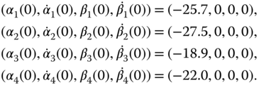
The initial states of the four helicopters are specified as follows:
Without loss of generality, the following non‐constant desired trajectories are adopted for experiments:
where all angles are given in degrees.
9.4.3 Control Strategies
Consider the directed communication topology graph shown in Figure 9.11. It is seen that only H1 has access to the desired trajectories, and Condition 3 is satisfied with ![]() , and all other entries of
, and all other entries of ![]() and
and ![]() are 0. Then, it follows that:
are 0. Then, it follows that:
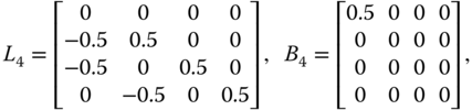
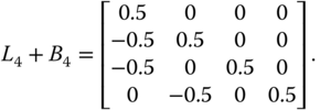
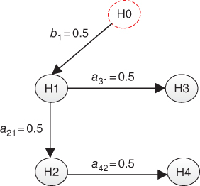
Figure 9.11 The communication topology for Experiments 2 and 3.
Consider the controller (5.19) with (5.20) and (5.32) for the motion synchronization of both elevation and pitch channels. Use ![]() and
and ![]() to denote the two entries of controller component
to denote the two entries of controller component ![]() ,
, ![]() and
and ![]() to denote the two entries of disturbance estimate vector
to denote the two entries of disturbance estimate vector ![]() ,
, ![]() and
and ![]() to denote the two entries of estimation error vector
to denote the two entries of estimation error vector ![]() ; that is,
; that is, ![]() ,
, ![]() , and
, and ![]() , where
, where ![]() .
.
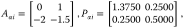
For the parameters of ![]() and
and ![]() , we choose
, we choose

which results in

where the subscripts ![]() and
and ![]() are added to the symbols introduced in Section , to distinguish the two channels.
are added to the symbols introduced in Section , to distinguish the two channels.
For comparison purposes, four experimental cases are studied. The same nominal controllers ![]() and
and ![]() with parameters as in (9.36) are applied for each case. The differences between these cases are:
with parameters as in (9.36) are applied for each case. The differences between these cases are:
- For Case 4, only
 and
and  are applied, which corresponds to the situation in Section and is equivalent to applying the controller (5.19) with
  ,
,  and
and  , to the four helicopters.
 - For Case 2, UDEs (5.32) with parameters
 and
and  are additionally applied for each helicopter.
 - For Case 3, UDEs (5.32) with smaller parameters of
 and
and  are applied for each helicopter, and none of the equipped ADSs are activated.
 - For Case 4, the same controllers as for Case 3 are applied, but the ADSs of helicopters 2 and 4 are activated.
In addition, for the controller design of each helicopter, the model parameters given in Table 9.1 are also used in this experiment, which is different from the situation considered in the above Experiment 1 (where the differences among the inertial parameters of the involved helicopters are explicitly considered). This implies that larger modeling errors are neglected in constructing the controller for Experiment 2, since, as shown in Table 9.2, ADSs on the helicopters lead to obvious uncertainties in the inertial parameters ![]() and
and ![]() .
.
9.4.4 Experimental Results and Discussions
9.4.5 Summary
To show the performance differences more explicitly, the maximum magnitudes of the tracking errors for the four cases are summarized and compared in Tables 9.4 and 9.5; the responses over the same time interval ![]() are considered in each case. From these tables, it is easy to see that both the tracking and synchronization accuracy improves if UDEs with smaller UDE parameters are used.
are considered in each case. From these tables, it is easy to see that both the tracking and synchronization accuracy improves if UDEs with smaller UDE parameters are used.
Table 9.4
Maximum tracking errors in elevation axis for ![]() s.
s.
| Case |
H1 ( |
H2 ( |
H3 ( |
H4 ( |
| 1 |
|
|
|
|
| 2 |
|
|
|
|
| 3 |
|
|
|
|
| 4 |
|
|
|
|
Table 9.5
Maximum tracking errors in pitch channel for ![]() s.
s.
| Case |
H1 ( |
H2 ( |
H3 ( |
H4 ( |
| 1 |
|
|
|
|
| 2 |
|
|
|
|
| 3 |
|
|
|
|
| 4 |
|
|
|
|
In this experiment, the UDE‐based robust synchronized tracking control of four 3‐DOF helicopters has been verified under the condition that only a small subset of the helicopters has access to the desired attitude information. This robust controller is obtained by augmenting a distributed tracker with a continuous disturbance estimator that produces a signal to compensate for the effect of disturbances involved in the actual dynamics. Experimental results demonstrate that both the tracking and synchronization accuracy are greatly improved by UDEs with suitable parameters, and that the smaller the UDE parameter is, the smaller the tracking errors and synchronization errors are.
9.5 Experiment 3: Output‐feedback‐based Sliding‐mode Control
9.5.1 Objective
The objectives of the experiment are:
- to design a robust controller by applying the sliding‐mode control approach proposed in Section for both elevation and pitch channels;
- to implement the controllers with or without disturbance compensation, and compare the performance;
- to check the control performance with respect to exogenous disturbances.
9.5.2 Initial Conditions and Desired Trajectories
The initial angular positions of the involved four helicopters are:
The initial angular velocities of all the helicopters is zero; that is, ![]() for each
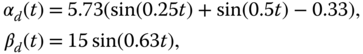
for each ![]() . The reference trajectory of angular position
. The reference trajectory of angular position ![]() is set to:
is set to:
so all the helicopters are expected to move sinusoidally in both channels, with amplitudes of ![]() and
and ![]() and frequencies of 0.15 Hz and 0.1 Hz for the elevation channel and pitch channel, respectively.
and frequencies of 0.15 Hz and 0.1 Hz for the elevation channel and pitch channel, respectively.
9.5.3 Control Strategies
Consider the same information‐exchange graph as shown in Figure 9.11 for this experiment. We apply and implement the controllers (5.79), (5.94), and (5.96) for the motion synchronization of both elevation and pitch channels.
The same nominal inertial parameters used in Experiment 2 are also used to construct the controller for the helicopters in this experiment, despite the fact that the differences among the parameters of the four helicopters are obvious. This in turn implies that the results obtained in this experiments also demonstrate the system's robustness with respect to the uncertainties in inertial parameters. Furthermore, by the definition of ![]() given by (5.18), one can see that the disturbance compensation term
given by (5.18), one can see that the disturbance compensation term ![]() reflects not only the effect of the disturbances and uncertainties of vehicle
reflects not only the effect of the disturbances and uncertainties of vehicle ![]() itself, but also that of its neighbors.
itself, but also that of its neighbors.
The controller gains for each helicopter are the same and given by:
These are tuned manually according to the response of the experiment, and the other parameters ![]() ,
, ![]() ,
, ![]() ,
, ![]() are accordingly determined using (5.116)–(5.119).
are accordingly determined using (5.116)–(5.119).
In addition, in order to attenuate chattering caused by the discontinuous signum function, we use standard saturation functions in the control law. The slope of the saturation functions is chosen as 1000.
9.5.4 Experimental Results and Discussions
For comparison purposes, three experimental cases are designed and implemented in this experiment, corresponding to different disturbance conditions or disturbance compensation strategies.
-
Case 1: the ADSs on helicopters 2 and 4 are turned off, and the control component
 is used for disturbance compensation for each helicopter.
 -
Case 2: the ADSs on helicopters 2 and 4 are turned on, and the control component
 is used for disturbance compensation for each helicopter.
 -
Case 3: the ADSs on helicopters 2 and 4 are turned off (as in Case 1), and the control component
 is removed from the implemented controller for each helicopter; in other words, the disturbance is not compensated for any helicopter.
9.5.5 Summary
In these experiments, the decentralized output‐feedback synchronized tracking control strategy, as developed in Section , was implemented and verified on a platform consisting of four 3‐DOF helicopters with only angular position measurements available. In particular, the effect of the disturbance compensation term ![]() included in controller (5.79) was evaluated.
included in controller (5.79) was evaluated.