Chapter 4. Introduction to Computations in Chemical Engineering

It is unworthy of excellent men to lose hours like slaves in the labor of calculation which could be safely relegated to anyone else if machines were used.

—Gottfried Wilhelm von Leibniz¹

1. Leibniz’s fame as the co-inventor of calculus overshadows his contributions in many other fields, including those in the field of computations. He was one of the earliest pioneers in the development of mechanical calculators. Quotation source: http://www-history.mcs.st-and.ac.uk/Quotations/Leibniz.html

Chemical engineering, like all engineering disciplines, is a quantitative field; that is, it requires accurate solutions of problems having high mathematical complexity. A chemical engineer must be able to model—develop quantitative mathematical expressions that describe the processes and phenomena—any system of interest, and simulate—solve the equations—the model. The solutions so obtained allow the engineer to design, operate, and control the processes. The courses described in Chapter 3, “Making of a Chemical Engineer,” provide the students with the theoretical basis for modeling the processes. The nature of the resulting equations and tools used for solving the equations are presented in this chapter.

The governing equations for the system follow:

Equations 4.1 and 4.2 state that the mole fractions of all components, numbering n, in each phase add up to 1. x_i and y_i represent the mole fractions of component i in the outlet liquid and gas phases, respectively. The mole fractions in the feed stream are denoted by z_i. (Typically, x is used to represent the mole fraction when the phase is liquid, and y is used when the phase is gaseous.) These two equations should be intuitively clear, as the mathematical statements of the concept that all fractions of any quantity must add up to the whole. Equation 4.3 is actually a system of n equations relating the mole fraction of a component in the gas phase to the mole fraction of the same component in the liquid phase. K_i is a characteristic constant for component i and is dependent on pressure, temperature, and the nature of the component mixture. Solution of this system of equations allows us to calculate the compositions of the two different phases, which is necessary for designing the separation scheme for the mixture. Each term in the system of equations is linear (variables having power of 1) in x or y.

A similar system of equations is used to model a stagewise gas-liquid contactor, such as a distillation column, described in Chapter 3. Figure 4.2 represents a distillation column containing N equilibrium stages [2]; the vapor and liquid inlet and outlet flows can be seen in the figure for stage k.

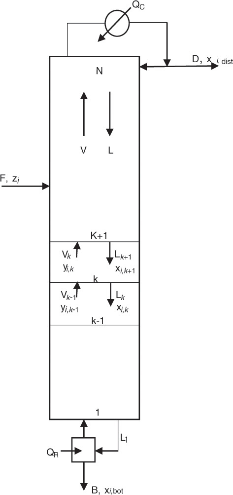
Source: Adapted from Wankat, P. C., Separation Process Principles, Third Edition, Prentice Hall, Upper Saddle River, New Jersey, 2012.

The material balances for each component yield the following system of n equations for stage k:

V and L represent the molar flow rates of the vapor and liquid stream, respectively. The subscripts for these flow rates represent the stage from which these flows exit. For example, V_k and L_k are the vapor and liquid flow rates exiting stage k, respectively. L_k+1 is the liquid flow rate exiting stage k + 1 and entering stage k, and V_k−1 is the vapor flow rate exiting stage k − 1 and entering stage k. The mole fractions are doubly subscripted variables, the first subscript representing the component, the second one the stage. Equation 4.4 is the mathematical representation of the steady-state nature of the system for each component: the amount of component i entering the stage through vapor and liquid flows is the same as the amount leaving through the exiting vapor and liquid flows. Each stage is assumed to be an equilibrium stage; that is, the exiting vapor and liquid flows are in equilibrium with each other. This allows us to utilize the equilibrium relationships of the form shown by equation 4.3 to complete the system description. The total number of equations for the entire column is N × n, which can be significantly large depending on the number of components present in the process stream and the number of stages needed to obtain the desired separation.

Algebraic equations encountered in chemical engineering can also be polynomial equations; that is, they can have variable orders greater than one. Equation 4.5 represents a typical polynomial equation of interest to chemical engineers:

This equation is an example of a cubic equation of state, V being the volume of the substance under the given conditions of temperature (T) and pressure (P). Constants a, b, c, and d are functions of the system pressure, temperature, number of moles, and fluid properties. An equation of state represents the relationship between the system temperature, pressure, and volume; the ideal gas law represented by the mathematical expression PV = nRT is the simplest of the equations of state. These equations of state are further used in thermodynamic calculations involving interconversion between energy and work, and phase equilibrium. It is readily apparent that an accurate equation of state is critical for superior process design and performance. Unfortunately, the volumetric behavior of most substances does not conform to the ideal gas law, and more complex equations are needed for accurately describing the P-V-T relationships for these substances. The cubic equations of state represent one of the developments addressing this need for improved accuracy. Equation 4.6 is an example of the cubic equation of state and is called the van der Waals equation [3].

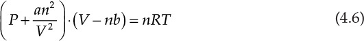
In this equation, a and b are constants characteristic of the substance, and n is the number of moles present in the system.

Several other more complex equations have also been developed, many of them polynomial in nature. A chemical engineering student encounters polynomial equations in practically every subject described in Chapter 3.

Re in the equation represents Reynolds number, a dimensionless quantity of enormous significance in fluid mechanics and transport phenomena. The Nikuradse equation allows us to calculate f, the friction factor, a quantity that further leads to the estimation of pressure drop for a flowing fluid and, ultimately, the power requirements for material transfer.

Equation 4.8 is another example of a transcendental equation that is used in the design of chemical reactors [6].

X_A represents the conversion (extent of reaction) of the reactant A, τ the residence time (the time spent by the fluid in the reactor), and A and E the characteristic parameters that describe the rate of reaction. The equation can be used to calculate one of the three quantities X_A, τ, or T when the other two are specified.

Many processes involve consecutive chemical reactions that can be represented by the equation A → R → S. A is the starting reactant, which upon undergoing the reaction yields the specie R, which is often the desired product. However, R may undergo further reaction forming S. The typical concentration profiles for the three species in a reactor as a function of time are shown in Figure 4.3. As can be seen, the concentration of A decreases continuously, while that of S increases continuously. The concentration of the desired product R increases first, reaches a maximum, and then starts decreasing. The concentration-time relationship for R when both the reactions are first order² with respect to the reactants is shown in equation 4.9 [7].

2. A first-order reaction is one in which the rate of reaction is proportional to the concentration of the reactant. These concepts are presented in more detail in Chapter 9, “Computations in Chemical Engineering Kinetics.”

Here, C_R is the concentration of R, C_A0 is the initial concentration of A, and k₁ and k₂ are the rate constants for the two reactions. Calculating the concentration of R at any specified time, when the rate constants and initial concentration of A are known, is straightforward. However, calculation of time needed to achieve a certain specified concentration of R is more challenging and requires use of techniques needed for the solution of transcendental equations.

Solution of this equation yields the concentration-time profile for the reactant A in the reaction, which provides the basis for the design of the reactor.

Higher-order differential equations are very common in chemical engineering systems. Figure 4.4 shows the cross-sectional view of a pipe conducting steam, the ubiquitous heat transfer medium in chemical plants. The pipe will inevitably be covered with insulation to minimize heat loss to the surroundings. Note that the heat loss can be reduced but not completely eliminated. Obviously, choosing proper insulation and determining the resultant heat loss is extremely important for estimating the energy costs. Heat loss can be calculated from the temperature-distance profiles existing in the system [5].

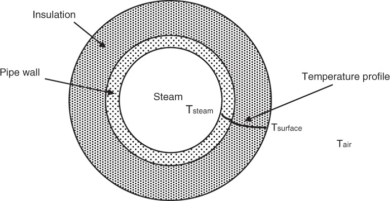
The governing equation describing the heat transfer for a cylindrical pipe follows:

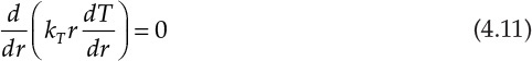
Equation 4.11 is a second-order ordinary differential equation that governs the relationship between temperature T and radial distance r from the center of the pipe. k_T is the thermal conductivity of the material, which depends on the temperature. As the temperature varies with respect to the radial position, the thermal conductivity is also a function of the radial position. Solution of this equation yields the temperature profile within that object, which in turn allows us to determine the heat lost to the surroundings.

The solution of differential equations requires specifying values of dependent variable(s) at certain values of the independent variable. These specifications are termed boundary conditions (at a specific location, with respect to dimensional coordinate) or initial conditions (with respect to time). Complete solution requires as many boundary/initial conditions as the order of the differential equation [4].

Frequently, modeling of a system leads to a set of ordinary differential equations, consisting of two or more dependent variables that are functions of the same independent variable. These equations need to be solved simultaneously to obtain the quantitative description of the system.

The concentration of the solvent within the film is a function of time as well as distance from the surface. Equation 4.12 is the fundamental equation³ for governing the solvent mass transport within the film, a partial differential equation that is first order with respect to time t and second order with respect to location x.

3. This is called the Fick’s second law equation.

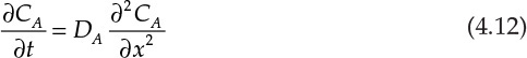
D_A is the diffusivity of solvent A in the polymer film, which depends on the properties of the system.

The solution of this (and other partial differential equations) requires an appropriate number of specifications (boundary and initial conditions) depending on orders with respect to the independent variables.

Here, F_A0 is the molar flow rate of species A, and −r_A is the rate of reaction, which is a function of conversion X_A. Equation 4.13 is represented by Figure 4.6, where the shaded region represents the integral and is equal to the quantity V/F_A0.

When the reaction rate cannot be easily integrated analytically, the shaded region—the area under the curve—is evaluated numerically.

To determine the rate constant k, experiments are conducted obtaining the concentration-time data and a linear regression carried out between ln(C_A) and t, as shown in Figure 4.7.

It can readily be seen that a chemical engineer must have skills to deal with and solve problems ranging from simple arithmetic calculations to those requiring highly sophisticated and involved algorithms. Further, the solution must be obtained fairly rapidly for the individuals and organizations to maintain their competitive edge and respond to changing conditions. Section 4.2 presents a brief overview of solution algorithms developed for numerical solutions of different types of problems. Section 4.3 describes the different tools including the machines and software available to chemical engineers to perform these computations.

In this equation, [X] is the column matrix of n variables; [A], the n × n matrix of coefficients; and [B], a column matrix of n function values.

The Gauss elimination technique for solving this system of equations involves progressive elimination of variables from the equations such that at the end only a single linear equation is obtained in one variable. The value of that variable is then obtained and back-substituted progressively into the equations in reverse order of elimination to obtain the values of the rest of the variables that satisfy equation 4.15. For example, if the system consists of n equations in variables x₁, x₂,…, x_n, then the first step is elimination of variable x₁ from equations 2 to n using equation 1 to express x₁ in terms of the rest of variables. The result is a system of n − 1 equations in n − 1 variables x₂, x₃,…, x_n. Repeating this procedure then allows us to eliminate variables x₂, x₃, and so on, until only an equation in x_n is left. The value of x_n is calculated, and reversing the calculations, values of x_n−1, x_n−2,…, x₁ are obtained [4].

Iterative procedures offer an alternative to elimination techniques. The Gauss-Seidel method involves assuming an initial solution by guessing the values for the variables. It is often convenient to assume that all the variables are 0. Based on this initial guess, the values of the variables are recalculated using the system of equations: x₁ is calculated from the first equation, and its value is updated in the solution matrix; x₂ is calculated from the second equation; and so on. The steps are repeated until the values converge for each variable [8]. The Gauss-Seidel method is likely to be more efficient than the elimination method for systems containing a very large number of equations or systems of equations with a sparse coefficient matrix, that is, where the majority of coefficients are zero [9].

Many sophisticated variations of the elimination and iteration techniques are available for the solution. One other solution technique involves matrix inversion and multiplication. The effectiveness of these and solution techniques is dependent on the nature of the system of equations. Certain techniques may work better in some situations, whereas it might be appropriate to use alternative techniques in other instances.

These equations are typically solved by guessing a solution (root) and refining the value of the root on the basis of the behavior of the function. The principle of the Newton-Raphson technique, one of the most common techniques used for determining the roots of an equation, is represented by equation 4.16 [4]:

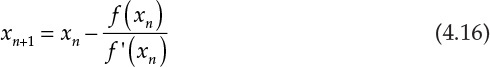
Here, x_n and x_n+1 are the old and new values of the root; f(x_n) and f’(x_n) are values of the function and its derivative, respectively, evaluated at the old root.

The calculations are repeated iteratively; that is, so long as the values of the roots do not converge, the new root is reset as the old root and a newer value of the root evaluated. It is obvious the new root will equal the old root when the function value is zero. In practice, the two values do not coincide exactly, but a tolerance value is defined for convergence. For example, the calculations may be stopped when the two values differ by less than 0.1% (or some other acceptable criteria).

The computations for this technique depend on not only the function value but also its behavior (derivative) at the root value. The initial guess is extremely important, as the search for the root proceeds on the basis of the function and derivative values at this point. Proper choice of the root will yield a quick solution, whereas an improper choice of the initial guess may lead to the failure of the technique.

The iterative successive substitution method can also be used to solve such equations [9]. The method involves rearranging the equation f(x) = 0 in the form x = g(x). The iterative solution algorithm can then be represented by the following equation:

Here, x_i+1 is the new value of the root, which is calculated from the old value of the root x_i. Each successive value of x would be close to the actual solution of the equation. The key to the success of the method is in the proper rearrangement of the equations, as it is possible for the values to diverge away from the solution rather than toward a solution.

Finding the roots of polynomial equations presents a particular challenge. An nth-order polynomial will have n roots, which may or may not be distinct and may be real or complex. The solution technique described previously may be able to find only a single root, irrespective of the initial guess. The polynomial needs to be deflated—its order reduced by factoring out the root discovered—progressively to find all the n roots. It should be noted that in engineering applications, only one root may be of interest, the others needed only for mathematically complete solution. For example, the cubic equation of state may have only one real positive root for volume, and that is the only root of interest to the engineer. A complex or negative root, while mathematically correct as an answer, is not needed by the engineer.

The subscripts refer to the time period. Thus, C_Ai is the concentration at time t_i, and so on. The derivative is approximated by the ratio of differences in the quantities. This formula is termed the forward difference formula, as the derivative at t_i is calculated using values at t_i and t_i+1. Similarly, there are backward and central difference formulas that are also applied for the calculation of the derivative [4, 10]. The comparative advantages and disadvantages of the different formulas are beyond the scope of this book and are not discussed further.

Similarly, the numerical techniques for integration of ordinary and partial differential equations are beyond the scope of this book. Interested readers may find a convenient starting point in reference [4] for further knowledge of such techniques.

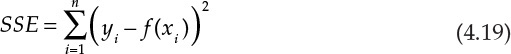
In this equation, y_i is the observed value, and f(x_i) is the predicted value based on the presumed function f. The function can be linear in a single variable (generally, what is implied by the term linear regression), linear in multiple variables (multiple regression), or polynomial (polynomial regression). Minimization of SSE yields values of model parameters (slope and intercept for a linear function, for example) in terms of the observed data points (x_i, y_i). The least squares regression formulas are built into many software programs.

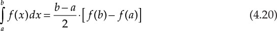
Decreasing the interval increases the accuracy of the estimate. Several other refinements are also possible but are not discussed here.

Section 4.3 describes various software programs that are available for the computations and solutions of the different types of problems just discussed. These software programs feature built-in tools developed on the basis of these algorithms, obviating any need for an engineer to write a detailed program customized for the problem at hand. The engineer has to know merely how to give the command in the language that is understood by the program. The previous discussion should, however, provide the theoretical basis for the solution as well as illustrate the limitations of the solution technique and possible causes of failure. A course in numerical techniques is often a required core course in graduate chemical engineering programs and sometimes an advanced undergraduate elective course.

A couple of tools developed in response to the ever-increasing demand for higher speeds worth mentioning are the log table and the slide rule. Figure 4.8 shows a page from the log table.

A log table enables all calculations, including highly complex ones, to be reduced to additions/subtractions, which can then be easily done by hand. The use of log tables is illustrated for the simple case of calculating the circumference C of a circle of diameter D. The concept and steps in calculations are as follows:

Equations 4.21, 4.22, and 4.23 demonstrate how a multiplication operation can be performed as an addition operation using the log tables. Logarithms of π and diameter are looked up in the log tables and added to obtain logarithm of the circumference. The answer is obtained by looking up the antilog of the sum in another set of tables.

The calculation will work with logarithms to any base; however, generally the tables are those of common logarithms (to the base 10) rather than natural logarithms (to the base e). An impressive compilation of common logarithms up to 24 decimal places of numbers leading to 200,000 was available by the end of the 18th century through the efforts of a large number of individuals.

Such compilations and early calculating machines were hardly portable, a disadvantage that was overcome by the slide rule. This elegant device was the size of a ruler and small enough to fit in a shirt pocket; a couple of examples are shown in Figure 4.9. As seen from the figure, a slide rule has a central sliding part, and both the fixed and sliding parts are marked with several scales. Multiplication, division, and logarithmic as well as trigonometric calculations can be rapidly performed using the slide rule, which became an indispensable tool for engineers until it was supplanted by inexpensive scientific calculators in the mid-1970s.

The advent of computers enabled engineers to perform highly complex, involved, repetitive calculations and improve the accuracy of solutions. Mainframe computers were ubiquitous by the 1950s, with engineers writing programs and submitting them as jobs to be run on the mainframes.

Rapid technological advances in memory and data storage, materials, and processors resulted in lowering the cost of computers, making them affordable to most people. By the mid-1990s, personal computers (PCs) had become ubiquitous and an essential accessory for an engineering student. Continual reduction in the cost and size of devices has resulted in the availability of portable devices such as laptops and tablets that allow us to perform practically all types of computations except for the most complicated ones that require the use of supercomputers.

Developed in the 1950s, Fortran (from formula translation) became the dominant programming language for scientific computing, and even today remains the preferred language for highly intensive computations of large systems. Each line of the Fortran program used to be transferred onto a card using a keypunch machine. (An IBM punched card with 80 columns is shown in Figure 4.10. Each number, letter, and symbol was represented by a hole or holes punched in the column [11]). A deck of such punched cards would constitute a program, which along with the necessary data would be submitted to be run as a job on the mainframe computer. Subsequent developments eliminated the need for punch cards, and a Fortran program can now be run on a personal computer, similar to programs in other languages.

Source: Ceruzzi, P. E., A History of Modern Computing, Second Edition, MIT Press, Cambridge, Massachusetts, 2003.

A large number of program modules developed over the past 60 years have resulted in a valuable library of programs in Fortran, and these modules are used every day throughout scientific and engineering computations.

Although Fortran remains indispensable for advanced computing, a large number of advanced software programs are available on the PC to perform most of the chemical engineering computations. The ubiquitous availability of these software programs has essentially eliminated the need for individuals to write their own software codes for all but only very specific problems [12]. Following are descriptions of a few of these software packages.

• Tools for solving algebraic and transcendental equations

• Graphing and regression tools

• Tools for solving iterative calculations

• Data and statistical analysis tools

Spreadsheets can be used to solve all types of computation problems, including differential and integral equations, described in section 4.1.

• Aspen Plus by AspenTech, Massachusetts, USA

• PRO/II by Invensys, Texas, USA (a division of Schneider Electric)

• ProSimPlus by ProSim, S.A., France

• CHEMCAD by Chemstations, Inc., Texas, USA

All of these software systems offer similar capabilities and user interfaces. A design engineer will invariably be using one of these environments for designing an operation, a unit, or the plant. Appendix B illustrates the capabilities of one of these software programs—PRO/II—for solving a complex separation problem to provide an idea of the amazing computational power at our disposal.

In addition to these general-purpose software programs, some specialized software for specific applications is also available, such as FLOTRAN/ANSYS (ANSYS Inc., Pennsylvania, United States) for pipe flow/fluid dynamics computations. Open source software such as Modelica (JModelica.org) is also available for modeling and simulation of complex systems.

2. Wankat, P. C., Separation Process Engineering, Third Edition, Prentice Hall, Upper Saddle River, New Jersey, 2012.

3. Kyle, B. G., Chemical and Process Thermodynamics, Third Edition, Prentice Hall, Upper Saddle River, New Jersey, 1999.

4. Chapra, S. C., and R. P. Canale, Numerical Methods for Engineers, Seventh Edition, McGraw-Hill, New York, 2014.

5. Welty, J. R., C. E. Wicks, R. E. Wilson, and G. L. Rorrer, Fundamentals of Momentum, Heat, and Mass Transfer, Fifth Edition, John Wiley and Sons, New York, 2008.

6. Fogler, H. S., Elements of Chemical Reaction Engineering, Fourth Edition, Prentice Hall, Upper Saddle River, New Jersey, 2006.

7. Doraiswamy, L. K., and D. Üner, Chemical Reaction Engineering: Beyond the Fundamentals, CRC Press, Boca Raton, Florida, 2014.

8. Rice, R. G., and D. D. Do, Applied Mathematics and Modeling for Chemical Engineers, Second Edition, John Wiley and Sons, New York, 2012.

9. Riggs, J. B., An Introduction to Numerical Methods for Chemical Engineers, Second Edition, Texas Tech University Press, Lubbock, Texas, 1994.

10. Pozrikidis, C., Numerical Computation in Science and Engineering, Second Edition, Oxford University Press, New York, 2008.

11. Ceruzzi, P. E., A History of Modern Computing, Second Edition, MIT Press, Cambridge, Massachusetts, 2003.

12. Finlayson, B. A., Introduction to Chemical Engineering Computing, Second Edition, John Wiley and Sons, New York, 2014.

4.2 The Newton-Raphson technique may not converge to a solution. Inspecting equation 4.16, in what other possible way can the technique fail?

4.3 Roots of any equation can be found using what is known as the bracketing technique. Conduct a literature search and explain the principle behind such solution techniques.

4.4 The following data were obtained in an experiment where the concentration of a substance was monitored as a function of time. Calculate the first derivative of the concentration with respect to time for all possible times using the forward difference formula. Can the second derivative also be calculated numerically?

4.5 What is the area under the concentration-time curve obtained from the data shown for problem 4.4? Use the trapezoid method. An alternative technique is to use the rectangle method. What is the difference in the areas if the area is calculated using the rectangle method?

References

1. Varma, A., and M. Morbidelli, Mathematical Methods in Chemical Engineering, Oxford University Press, Oxford, England, 1997.