
Appendix A. Introduction to Mathematical Software Packages
Chapter 4, “Introduction to Computations in Chemical Engineering,” introduced a variety of mathematical problems encountered by a chemical engineer in his/her academic and professional career. Chapters 5 through 9 presented some of these problems and computations executed using Excel and Mathcad. Excel is, of course, ubiquitous on personal computers as a part of the Microsoft Office Suite. The other software, Mathcad, is not as universally available. Nevertheless, several other software packages that can offer comparable capabilities are invariably available, both in academic institutions and organizations beyond. All these packages offer exceptional PC-based computational power to solve practically any problem in the chemical engineering field. These software packages have essentially eliminated any need for an individual to develop customized programs in a higher-level computer language (such as Fortran) by developing specific tools to address particular computational needs [1]. A brief introduction to other software packages (apart from Mathcad) is provided in this appendix. These packages include POLYMATH (www.polymath-software.com), MATLAB (www.mathworks.com/products/matlab), Maple (www.Maplesoft.com), and Mathematica (www.Wolfram.com). This appendix includes a solution of one of the example problems discussed in Chapter 9, “Computations in Chemical Engineering Kinetics,” using two of these software packages, followed by a brief comparative discussion of some of the salient features of the packages.
A.1 Example 9.2.2 Revisited
Example 9.2.2 involved determining the conversions in an adiabatic continuous stirred tank reactor (CSTR) by solving the mass and energy balance equations simultaneously. The problem is restated here:
The material balance and energy balance for a CSTR for a first-order reaction are given by equations A.1 and A.2, respectively. What is the conversion in the reactor? What is its operating temperature?


Here, CPA is the mean specific heat capacity of the reactor contents. ![]() is the mean residence time of the material in the reactor—that is, the time it spends in the reactor—obtained by dividing the reactor volume by the volumetric flow rate (V/v). T0 is the inlet temperature (temperature of the feed stream). XEB and XMB are the conversions using the energy balance and the material balance on the reactor, respectively. ΔHrxn is the heat of reaction.
is the mean residence time of the material in the reactor—that is, the time it spends in the reactor—obtained by dividing the reactor volume by the volumetric flow rate (V/v). T0 is the inlet temperature (temperature of the feed stream). XEB and XMB are the conversions using the energy balance and the material balance on the reactor, respectively. ΔHrxn is the heat of reaction.
The data for the reactor are as follows:
T0 = 293 K, CPA = 810 J/mol K, ΔHrxn = −200 kJ/mol, V = 10 L,
v = 0.2 L/s A = 1.8 × 10⁵ s−1, Ea = 50 kJ/mol
The solution technique for the problem using Mathcad was illustrated in Chapter 9. Readers should by now be familiar with the technique to solve the problem using Excel, so that solution is not discussed here. Solutions using POLYMATH and MATLAB are presented in the following sections. The installation of these programs on PCs is a straightforward matter and hence is not discussed here. The program is launched as any other program installed on a PC, by clicking on the icon or selecting from the list of programs.
A.1.1 POLYMATH Solution
Launching the POLYMATH program brings up the screen shown in Figure A.1.
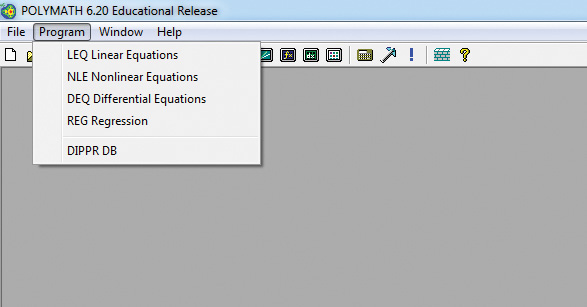
As can be seen from the figure, POLYMATH can be used to solve linear equations, nonlinear equations, and ordinary differential equations as well as perform regression analysis—the options are available under the Program command. The last option seen, DIPPR DB, refers to the database of physical properties through the Design Institute for Physical Properties (DIPPR) of the American Institute of Chemical Engineers (AIChE). The example problem involves a nonlinear equation, and hence that option is chosen from the Program command dropdown menu.
Clicking the NLE Nonlinear Equations option brings up another screen in POLYMATH where users can enter the needed equations. The nonlinear equations are entered by clicking on the appropriate icon, which brings up a dialog box where the equation can be entered as a function of the variable to be solved for. The problem specification typically requires a number of other auxiliary linear equations to be entered (such as those providing the data for the problem), and these can be entered by clicking the icon for auxiliary equation or by simply typing the equation.
Once all the equations are entered, lower and upper limits are specified for the variable, and the program is run by clicking the Run icon or by selecting it from the menu. The user can select an option to draw a graph of the solution. This procedure was followed for the example problem, and the resultant solution is shown in Figure A.2.

Figure A.2 POLYMATH solution to example 9.2.2.
The salient features of the procedure and solution are as follows:
1. The data are entered as auxiliary equations by simply typing a variable name and its value.
2. The nonlinear equation is entered as a function of temperature. The function is entered as f(T) = XMB − XEB. (Here, XMB and XEB represent the right hand sides of equations A.1 and A.2, respectively, as seen from the two equations and Fig. A.2).
3. A search space is defined by specifying the minimum and maximum temperatures.
4. POLYMATH performs the computations and plots the function as shown in the plot. It can be seen that the function value is 0 at three temperatures.
5. In addition to the graph, POLYMATH outputs the three temperature values. Two of the three solutions are visible in the figure. The third solution (solution #3 of 3) is ~538 K, the same as that obtained using Mathcad. The conversion is 0.99 at this temperature.
A.1.2 MATLAB Solution
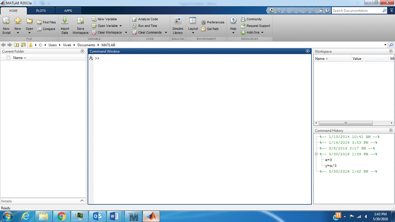
Launching the MATLAB program brings up the screen shown in Figure A.3. The opening screen of MATLAB is considerably more detailed than those of the other programs encountered until now. The menu bar has a number of icons and options, and the workspace is divided into four areas. The largest area is titled Command Window, and this is the main workspace for entering data and instructions. The space to the left deals with the organization of the files and folders, and the two spaces to the right contain the information about the current problem being worked on. This information involves a command history at the bottom and the tracking of variables above it.
The problem is solved by entering the values of the variables—the specified data for the problem. Once all the values are entered, the solution is obtained by typing the following line:
T=solve(A*exp(-Ea/R/T)*(V/v)/(1+A*exp(-Ea/R/T)*(V/v))==CPA*(T-T0)/(-DHrxn))
The variables correspond to the stated specifications. The command for the solve function involves equating the conversion from the material balance equation to the conversion from the energy balance. A double equal-to operator (==) is used in the solve function. MATLAB yields a solution of 537.4 K as the reactor temperature. The conversion at this temperature is 0.99, the same as that obtained using Mathcad and POLYMATH. The solution procedure and the solution are shown in Figure A.4.

Figure A.4 MATLAB solution to Example 9.2.2.
The commands entered can be seen in the Command window. The window to the bottom right contains the command history, and the variables and their values can be seen in the window above it. The window to the left of the Command window contains the names of the files and folders.
Creating plots in MATLAB requires a slightly more involved procedure. First, the temperature variable is defined with a range of values. Then, two function files are created, which define and evaluate XMB and XEB as functions of the temperature. The details of defining a range for the temperature variable and creation of the two functions are not shown here and are left to the reader to explore. The plots of XMB (conversion from mass balance) and XEB (conversion from energy balance) as a function of temperature are then created by entering the following command:
PLOT(T, XMB, T, XEB)
This command creates the plot shown in Figure A.5.

It should be noted that alternative solution techniques for this example are possible in MATLAB. In any case, it can be seen that all three software programs (Mathcad, MATLAB, and POLYMATH) yield nearly identical solutions to the problem. Readers can verify for themselves that other programs (Excel, Mathematica, Maple, or any other program they employ for solving the problem) also yield the same results. The following section presents a brief comparison of the software packages.
A.2 Comparison of Software Packages
All the software packages offer some basic capability for computations, and then each one has its own unique features. An overview of similarities and differences is described in the context of various operations, such as basic arithmetic calculations, graphing, and programming capabilities.
A.2.1 Variables and Basic Operations
All the programs allow variables to be defined, and variable names are, in general, unrestricted. (Typically, computations in Excel reference the cell containing the variable; however, it is possible to assign a variable name.) All programs have built-in definitions of many variable names but also have provisions for overriding this definition. For example, MATLAB defines both i and j as √–1, but a user can assign a different value to them [2]. Similarly, Mathcad has built-in units and symbols: for example, by default, letters A, V, and L carry specific meanings of ampere, volt, and liter, respectively. However, the user can redefine these as variables to represent area, volume, length, or any other quantity [3]. Each program uses different syntax for assigning values to variables or defining the variable. For example, Mathcad uses a colon (:) as the assignment operator, whereas Maple uses a colon followed by equal to sign (:=) for assignment [3, 4]. Other programs use a simple equal-to sign (=) for assignment, whereas Mathcad uses it for evaluation and obtaining output. With practice, a user can gain expertise and use proper syntax. Most programs also provide color-coded errors and warnings if improper syntax or undefined variables are used in command or computation statements. Some programs have built-in units, such as SI units in the case of Mathcad, by default. For example, the default unit for pressure is Pa (pascals), and the values of any pressure variable will be output in this unit in Mathcad. Mathcad also has automatic conversion facilities for displaying the variable values in any user-chosen units. The user can simply click on the unit, change it to the desired unit (atm or psi, for example), and Mathcad will automatically recalculate and display the proper number. Other programs require manual conversion of units.
All the programs use the same symbols (+, −, *, /) for arithmetic operations. Almost all programs allow a variable to be defined as a multidimensional array. In fact, most of the variables in MATLAB are considered as matrices (MATLAB stands for Matrix Laboratory) [2]. Most programs permit matrix computations and display error codes if invalid operations are attempted (addition of matrices of different dimension, etc.). All software programs have built-in functions for computing logarithms, trigonometric functions, and so on.
A.2.2 Equation Solving, Symbolic Computations, Plots, and Regression
All the programs have the capability to solve systems of linear algebraic equations as well as nonlinear transcendental equations. Excel offers this capability through its Goal Seek and Solver tools, and POLYMATH has its LEQ and NLE solvers. Solution techniques for Mathcad and MATLAB are presented in the book and in this appendix. Similar capability exists in Maple and Mathematica as well. Of course, each program may have multiple alternative pathways to arrive at the solution of the problem. A user, with practice, can master different techniques for solving problems. All programs also have the capability for solving many ordinary differential equations simultaneously. For example, POLYMATH has the DEQ program utility for solving differential equations, with initial conditions specified. Excel does not have a similar tool for solving differential equations; however, the grid structure of Excel makes it possible to manipulate the cells to adapt any numerical solution technique for ordinary as well as partial differential equations. Mathcad, MATLAB, Maple, and Mathematica also allow symbolic computations, such that users can obtain derivatives and integrals of expressions.
All programs have a graphing utility to generate plots—two-dimensional and, in some cases, three-dimensional. All programs have tools to manipulate the appearance of the graphs, including the color and shape of lines, markers, legends, axes scales, labels, and other elements. The ease of creation of plots and manipulating the format varies with the program, but users can easily learn to use the tools to enhance the effectiveness of the plots.
All programs also have regression tools for carrying out linear and nonlinear regression. The output of these tools generally includes statistical information about the goodness of fit and confidence in the estimates of the model parameters. Again, as with the plotting tools, users can acquire sufficient dexterity with practice.
A.2.3 Programming
Most of the computational problems encountered by a chemical engineer can be solved using any one of these programs (as well as some others not discussed in this appendix or the book). As mentioned earlier, the need to develop a customized program in a high-level language has been reduced considerably in recent times, primarily due to advances in the tools available in these software packages. However, a customized program may be needed for conducting computations in certain situations. Nearly all the software packages offer this programming capability, which is perhaps the biggest differentiating characteristic among these packages.
Excel offers a programming environment through its Excel VBA (Visual Basic–based) environment. Users can write the necessary programs (macros) and execute them for obtaining solutions. Although the programming capability in POLYMATH is limited, the POLYMATH outputs and statements can be converted and exported into MATLAB programs.
All other software packages offer the programming capability to varying degrees. All software packages have similar basic structure, with repeated calculations in loops, with for, if, and while statements serving as loop flow control tools. The versatility of programming is perhaps higher with MATLAB and Mathematica than with Maple and Mathcad.
Apart from these basic capabilities, each software package may contain specialized features that are suitable for many other applications. For example, Figure A.6 shows some of the tools available in MATLAB; the screen is brought up by clicking the APPS tab in the opening screen.

These apps provide MATLAB capabilities in signal processing, tuning of controllers, neural net fitting, optimization, and so on. These capabilities may be useful to a chemical engineer in some situations.
A.2.4 User Interface and Ease of Use
A fairly important consideration, particularly for a novice user, is the interface offered by the program and the ease of operation. The familiarity of Excel makes its interface one of the easiest to work with. The POLYMATH interface is equally friendly: it is not overloaded with icons and options, and it provides easy access to the particular computational problems (linear equations, differential equations, etc.). POLYMATH requires possibly the least amount of training, and a minimal time delay for a user to start wielding the computational tools. Of the remaining four, Maple and Mathcad have simpler, user-friendly interfaces, and MATLAB and Mathematica have comparable, more complex interfaces.
It should be noted that the programs with more complex interfaces also offer more capabilities with respect to programming and integration with other applications. An individual, with sufficient time and practice, can and will find the interface to be convenient. However, there is a significant learning curve for advanced software programs while the user gains familiarity with the syntax and command structure that is not intuitively clear [5]. The Help documentation offered by all of the programs is useful to a varying degree, with Excel and POLYMATH Help being the most useful, and MATLAB being less user friendly.
A.3 Summary
A large number of software programs ranging from the ubiquitous Excel to Mathematica and MATLAB are available in the market for performing engineering computations. In general, all the programs discussed in this appendix are effective in solving most of the computational problems encountered by a chemical engineer, such as the example problem of Chapter 9. A brief comparison of the capabilities of the various programs indicates that most of these programs offer similar computational capabilities. The comparison presented in this appendix is not intended to be comprehensive in nature, and many differences exist in the details of the features and executions. The software packages do differ in terms of their programming capabilities, and individuals who expect to or need to develop customized programs should explore these capabilities in detail before selecting a software package to procure.
References
1. Cutlip, M. B., J. J. Hwalek, H. E. Nuttall, M. Shacham, J. Brule, J. Widmann, T. Han, B. Finlayson, E. M. Rosen, and R. Taylor, “A Collection of 10 Numerical Problems in Chemical Engineering Solved by Various Mathematical Software Packages,” Computer Applications in Engineering Education, Vol. 6, No. 3, 1998, pp. 169–180.
2. Constantinides, A., and N. Mostoufi, Numerical Methods for Chemical Engineers with MATLAB Applications, Prentice Hall, Upper Saddle River, New Jersey, 1999.
3. Adidharma, H., and V. Temyanko, Mathcad for Chemical Engineers, Second Edition, Trafford Publishing, Victoria, British Columbia, Canada, 2009.
4. White, R. E., and V. R. Subramanian, Computational Methods in Chemical Engineering with Maple, Springer-Verlag, Berlin Heidelberg, Germany, 2010.
5. Cutlip, M. B., and M. Shacham, Problem Solving in Chemical Engineering with Numerical Methods, Prentice Hall, Upper Saddle River, New Jersey, 1999.