6.1 Introduction to reserves

Given an insurance or annuity contract and a duration k, the reserve at time k is defined exactly as in Definition 2.7. It is the amount that the insurer needs at time k in order to ensure that obligations under the contract can be met. Calculating reserves for each policy is an important responsibility of the actuary, known as valuation. The insurer wants to be confident that funds on hand, together with future premiums and investment earnings, are sufficient to pay the promised future benefits. It is important to thoroughly master the concept of insurance and annuity reserves in order to properly understand and analyze the nature of these contracts.

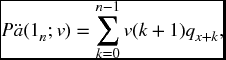
Throughout this chapter we will deal with the following model. As usual we start with a fixed investment discount function v and a life table. We have a contract issued on (x) with death benefit vector b, annuity benefit vector c and premium vector π. (For simplicity we will omit the possibility of guaranteed payments in our discussion, but this feature can easily be incorporated if desired.) Recall from Section 5.5 that we can view the death benefits as a vector of annuity benefits b*w_x, where (w_x)_k = v(k, k + 1)q_{x + k}. We can then form the net cash flow vector

(6.1)

which indeed represents the net cash flow on the contract from the insurer’s viewpoint. The insurer will collect premiums of π and pay out death benefits in the form of b*w_x and annuity benefits of c. The reserve at time k on the contract is the reserve for the vector f with respect to the interest and survivorship discount function, as given in Definition 2.6. Denoting the reserve by _kV, we have

(6.2)‡

It is often useful to write this in an alternate way that keeps benefits and premiums separate. That is, we note that the reserve at time k is the value at time k of future benefits less the value at time k of future premiums. This can be written in terms of the standard A and symbols as

(6.3)

or, equivalently (and the way in which it usually appears in the literature) as

(6.4)

Here we are using (4.8) and the corresponding statement for A.

Under the assumption that premiums are actuarially equivalent to benefits, we can also calculate the reserve retrospectively as

(6.5)

Under this formulation the reserve is the value at time k of the past premiums less the value at time k of past benefits. The reader is cautioned that the reserve cannot be so calculated when premiums and benefits are not actuarially equivalent.

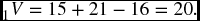
Example 6.1 For the policy of Example 5.5, find the reserves at time 1 and time 2. See Figure 6.1. As in Chapter 2 we use an arrow to mark the point at which values are computed.

Solution.

• Value at time 1 of future death benefits = 75(1/2)(0.4) = 15.
• Value at time 1 of future annuity benefits = 70(1/2)(0.6) = 21.
• Value at time 1 of future premiums = 16.
  

The above approach is recommended for hand calculation. All reserve calculations can be handled in exactly the same way, although there will generally be more than one summand in each of the three items.

Additional information can be obtained by first computing the net cash flow vector, which also provides the best procedure for spreadsheet calculation. To illustrate, the vector w₆₀ = (0.1, 0.2, −). (We don’t have information to compute the third entry but it is irrelevant, since it is multiplied by 0.) Then, b*w₆₀ = (8, 15, 0), c = (0, 0, 70), π = (16, 16, 0), so that the net cash flow vector f is (8, 1, −70). For present purposes, we can forget about the particular death benefits and premiums. From the insurer’s viewpoint the contract can be viewed as simply one of collecting 8 at time 0, 1 at time 1, and paying back 70 at time 2. From (6.6), ₁V is just the negative of the value at time 1, with respect to interest and survivorship, of the payments at times 1 and 2. This equals −1 +70(0.5)(0.6) = 20, as above.

Similarly, ₂V is just the value at time 2 of the payment at time 2 which is 70. In general, for a contract running for n years, the reserve at time n is just the payment due at time n to the survivors. (Recall that from the convention introduced in Chapter 1, reserves are calculated before this payment.) For n-year term insurance, when there is nothing payable to survivors at the end, the nth year reserve will equal to 0.

Since we have used net premiums, we can calculate balances as a check.

which agree with our previous calculations.

The following example exhibits a point of interest.

Example 6.2 For a 4-year endowment insurance on (60), b₂ = 100, b₃ = 200 and there is a pure endowment of 200 paid at age 64 if the insured is then alive. You are given that π₂ = 10, π₃ = 20, q₆₂ = 0.1. The interest rate after 2 years is 25%. Find ₂V and ₃V. See Figure 6.2.

Solution.

• Value at time 2 of death benefits = 100(0.8)(0.1) + 200(0.64)(0.9)q₆₃.
• Value at time 2 of annuity benefits = 200(0.64)(0.9)p₆₃.
• Value at time 2 of premiums = 10 + 20(0.8)(0.9) = 24.40.

We don’t know q₆₃, but it is not needed. Since q₆₃ + p₆₃ = 1, the two unspecified terms sum to 200(0.64)(0.9) = 115.20 and

Similarly, ₃V = 200(0.8) − 20 = 140.

This example shows that for an endowment insurance (with benefits paid at the end of the year of death) where the pure endowment is the same amount as the final death benefit, we do not need to know the mortality rate for the final year. This is in fact evident, since the insured gets that amount whether they live or not.

Remark There is a subtle point involved with Equation (6.6), which is important to note for the actual calulation of reserves. We have already introduced the idea in Section 2.10.3. In our model we choose an investment discount function and a mortality table, and these remain fixed for the duration of a contract. In practice, when one reaches time k and actually wants to compute _kV these assumptions may well have changed. The reserve computed at time k will be

where the primes indicate quantities that are calculated with the new interest and survivorship function y′_{x + k} as computed under what could be changed conditions at time k. Of course when there is no change in assumptions, y′_{x + k} will just equal y_x  k and formula (4.6) shows that both formulas are the same. The point is then, that in practice, one does not really know what _kV will be before time k. In this more realistic setting, we can view the original formula (6.4) as the best estimate one could make of _kV, if asked to compute it at time 0.

6.2 The general pattern of reserves

Are insurance reserves generally positive or negative? Paradoxically, we will motivate the answer to this question by providing an example where they are neither.

Example 6.3 An insurance policy provides a death benefit of 1 paid at the end of the year of death. Level annual premiums are payable for life. The interest rate is constant and the value of q_x is a constant q for all x. Find the reserves and give an explanation for the answer.

Solution. Let p = 1 − q be the constant value of p_x. Then _kp_x = p^k, which is never 0. There is a positive probability of living to any age, so we have an example in which ω = ∞. Our vectors will be of infinite length.

Let v denote the constant value of v(k, k + 1). Then w_x is a vector with a constant entry of vq and the premium pattern vector ρ is a vector with a constant entry of 1. The net level premium π is clearly vq, since that will make the vectors w_x*b and π not only actuarially equivalent but actually equal to each other. The net cash flow vector f is then not just a zero-value vector but actually equal to the zero vector. All reserves will be 0.

What is happening here is that the premium of vq, collected each year, will accumulate to q at the end of the year, and this will be exactly sufficient to pay the death benefits due at that time. There will be nothing left over, so balances, and therefore reserves, equal zero.

The situation above is typical for many forms of insurance, such as automobile or property coverage, and insurers of such risks have little in the way of reserves. The given scenario is, however, not realistic for life insurance. The values of q_x are not constant but increase with age. If one paid for the insurance 1 year at a time, the yearly premium per unit of vq_x would rapidly increase and eventually become prohibitively high. As we noted in Chapter 5, the typical life insurance policies will level the premiums out. In most cases, policyholders are paying more in premiums than they need to in the early years, but not enough in the later years. At any point of time after time zero, future premiums will not be sufficient to cover the remaining benefits. The excess collected in the early years is used to cover this deficit. It is expected therefore that reserves are usually positive. This has important implications for the life insurance industry. It means that investing becomes a major activity, as life insurance companies tend to accumulate large amounts of assets. Some critics, with little understanding of insurance, look at these holdings of real estate, stocks and bonds, and claim that they represent unfair profits made at the expense of the policyholder. The truth is, however, that a large portion of these assets represent reserves, which in effect belong to the policyholders, as they will be used to pay the future benefits.

Negative reserves can arise on policies where the cost of the insurance benefits is decreasing each year. An example is a policy with a rapidly decreasing benefit amount, where despite the increase in q_x, the quantity b_kv(k, k + 1)q_{x + k} decreases. Some examples appear in the exercises. Similarly, negative reserves can arise in the case where the premiums increase rapidly rather than remaining level. Insurers try to avoid such a situation if possible. A negative reserve means, viewing things prospectively, that the policyholder owes money to the insurer, which will be provided by future premiums, or equivalently, looking at things retrospectively, that the policyholder has received coverage but not yet paid for it. The problem is that the policyholder may stop paying premiums on the policy, leaving an unpaid debt.

6.3 Recursion

In this section, we develop some important recursion formulas. It is convenient to make a slight alteration in notation. We will incorporate the annuity payments with the premiums and let π denote π − c. In other words, we think of annuity benefits as just negative premiums, which is really what they are, since the policyholder is receiving rather than paying these amounts. Our net cash flow vector f has entries f_k = π_k − b_kv(k, k + 1)q_{x + k}, and from our basic recursion formula (2.2),

(6.6)

Since y_x(k + 1, k) = (1 + i_k)/p_{x + k} this is sometime written as

(6.7)

The recursion is started with the initial value which will be 0 under our standard assumption of net premiums.

It is instructive to note that the last term of q_{x + k}/p_{x + k} is equal to d_{x + k}/ℓ_{x + k + 1}. From this, we see easily that it is the amount, per unit of death benefit, that each survivor must pay at the end of the year to provide the benefits paid to those who died during the year.

Formula (6.7) takes a retrospective viewpoint, and says that the reserve at time k + 1 is obtained from that at time k, by adding the premium, accumulating at interest and survivorship for 1 year, and then subtracting enough to pay the death benefits. It is known as the Fackler reserve accumulation formula, named after one of the early North American actuaries, David Parks Fackler. In pre-computer days it was a popular method for calculating reserves. It is used infrequently for calculating purposes now, but is still useful for illustrating how the life insurance reserve changes from one period to the next.

Remark The quantity _kV + π_k in the above formula is often called the initial reserve at time k as it represents the reserve at the beginning of the year, after the payment of the premium. In contrast, _kV is sometimes referred to as the terminal reserve at time k, reflecting the fact that it the reserve at the end of the year, prior to the payment of the premium for the following year.

Alternate versions of this formula provide instructive information. We first give an important definition.

Definition 6.1 The quantity b_k − _{k + 1}V is known as the net amount at risk for the (k + 1)th year and will be denoted by η_k (the subscript is chosen to correspond to b_k). (There are various other names in the literature, such as death strain at risk.)

Now, multiplying (6.7) by p_{x + k} = 1 − q_{x + k} and rearranging, we get

(6.8)

Formula (6.8) reflects the fact that we can also view the accumulation of funds on an insurance policy as an interest-only investment, rather than as an interest and survivorship investment. From this point of view, the policyholder keeps the reserve when he/she dies (the amount accumulated in her box), but then the insurer only needs to make up the difference as a death benefit. The insurer is therefore at risk only for the difference between the death benefit and reserve, which is the source of the name.

Readers who looked at Section 2.11 will note that this is a special case of the change of discount function that we investigated there. In this case y_x and b_k are replaced by v and η_k, respectively.

6.4 Detailed analysis of an insurance or annuity contract

In this section we use (6.8) to provide a detailed discussion of the workings of an insurance policy.

6.4.1 Gains and losses

In practice, interest and mortality rates will not conform exactly to those provided by our model. In a particular year, the insurer may earn more interest than predicted by the given discount function, which will result in gains. For an insurance contract, there may be fewer deaths than predicted by the given life table, also causing gains. If the insurer earns less interest than expected, and/or there are more deaths than expected, there will be losses. In any year, the actuary wants to analyze these gains or losses and see how much is due to investment earnings and how much is due to mortality.

Suppose we wish to measure the gain for a particular policyholder over the period running from time k to time k + 1. At the beginning of the year, before premium payment the policyholder’s box will contain the amount _kV. At the end of the year the insurer must make certain that the box has _{k + 1}V in order that future obligations can be met. Anything in excess of that amount can be considered as a gain, taken out and added to general surplus funds. On the other hand, if there is less than _{k + 1}V, the insurer will have to make up the deficit from general surplus funds and there will be a loss. We will derive some general formulas. Suppose the actual interest rate earned during this year was i*_k rather than i_k, and the actual rate of mortality was q*_{x + k} rather than q_{x + k}. Then, the actual amount accumulated at time k + 1 will be the right hand side of (6.8) with starred i and q. If we subtract the reserve, we obtain the total gain G_k from that policy for that year as

(6.9)

If we substitute for _{k + 1}V with the left hand side of (6.8) we can write this as

(6.10)

which gives us a decomposition of the gain by source. The first term gives the gain due to mortality, and the second term gives the gain due to interest. That is, the mortality gain is the difference between the expected and actual mortality rates times the net amount at risk. The interest gain is the difference between actual and expected interest rates times the amount of funds at the beginning of the year, after payment of the premium.

Example 6.4 Refer back to the policy of Example 6.1. Suppose that in the first year of the policy, the interest earned was 50% instead of the predicted 100%, and the actual rate of mortality was 0.1 instead of the predicted 0.2. Find the total gain for the year, split into the portion due to interest and the portion due to mortality.

Solution. Substituting directly from (6.6), the mortality gain is

while the interest gain is

There is a total gain of −2, or in other words a loss of 2, for each policy.

We will verify this by working out an example in the aggregate. Suppose that 10 people age 60 buy this policy at a certain time. The insurer collects 160, and this accumulates at 50% interest to 240 at the end of the year. Out of this, the insurer will pay a death benefit of 80 for the one death that occurred, leaving a total of 160. They have to put aside a total of 180, which is the reserve of 20 for each of the 9 survivors. There is a aggregate shortfall of 20, or 2 from each policy, which has to be drawn from surplus. (Note that the gain given by (6.8) is for each policy in force at the beginning of the year, not at the end.)

Formula (6.9) assumes that the premium paid is the net premium, calculated as in Chapter 5. In practice, the premiums actually charged on a policy will normally be different from the valuation premiums which are net premiums determined from the interest and mortality assumptions used to compute reserves. (See Section 6.5 for more detail on this.) This necessitates an adjustment in our analysis. Suppose the premium paid at time k is actually π*_k rather than valuation premium π_k. The first term on the right of (6.8) is then

which leads to an extra source of gain or loss. We now have

(6.11)

The third term represents the gain or loss arising from premiums that differ from the valuation premium. (We will elaborate on this point in Section 12.4.)

One application of the formulas in this section is to dividend calculation. Insurers frequently issue what are termed participating policies, in which gains resulting from favourable investment and mortality experience are returned to the policyholder in the form of dividends. We will not go into further detail on this topic, but note that formula (6.10) is a basic tool in computing these amounts.

Another use of gain and loss analysis is to determine how changes in the basis assumptions will affect the reserves. As an example, suppose that the reserve interest rate decreases. It is clear that valuation premiums will increase. In order to provide the same benefits with decreased earnings from investments, more must be collected from the policyholder. On the other hand, it is not clear how this will affect reserves, since at any time, both the present value of the future benefits and the present value of the future premiums will increase. Indeed, the effect will depend on the nature of the policy. In the usual case however with a level premium π and reserves that increase with time, the lowering of the interest rate will increase reserves. To see this, suppose that interest rates are constant and there is a change of rate from i to i* < i. This will cause an interest loss of (_kV + π)(i − i*) for the year running from time k to k + 1. Since the reserves are increasing with time, the losses will also be increasing with time. There will be of course a new level valuation premium of π + Δ to cover these losses. Due to the increasing losses, it must be that Δ is greater than the losses in early years and less in later years. In the early years, that portion of Δ not used to cover the loss, will be set aside as an extra reserve, to cover the greater losses to come in the future, and this will cause reserves to increase.

6.4.2 The risk–savings decomposition

We now look at a useful decomposition of the policy into a risk portion and a savings portion. Multiply Equation (6.8) by v(k, k + 1) and rearrange to obtain

This formula decomposes each premium into two parts. The first term is known as the risk portion of the premium, as it is that amount needed to buy insurance for 1 year for the net amount at risk. The remainder provides for the difference in reserves and is known as the savings portion of the premium.

Example 6.5 Find the decomposition for the premiums of Example 6.1.

Solution. In the first year the net amount at risk is 80 − 20 = 60. The risk portion of the premium is then . The savings portion is . (As a check, the two portions add up to the total premium.) In the second year the net amount at risk is 75 − 70 = 5. The risk portion of the premium is and the savings portion is .

This decomposition shows that any policy can be viewed as being composed of two separate policies, the pure insurance part and the savings part.

For the pure insurance part, the premium is the risk premium and the death benefit paid is the net amount at risk. This part of the policy has zero reserves, as the risk premium is just sufficient to purchase coverage for the net amount at risk for 1 year. In the above example, the policyholder pays 6 in the first year, which is exactly enough to purchase the coverage for the net amount at risk of 60. He/she then pays 1 in the second year, which is exactly enough to purchase coverage for the net amount at risk of 5.

The savings part of the policy operates just like a bank account, with amounts accumulating at interest only. In the example above, the savings portion of 10 from the first premium accumulates to 40 at time 2 and the saving portion of 15 from the second premium accumulates to 30 at time 2. The total savings of 70 are then paid out as the pure endowment to all survivors at time 2. This is typical of endowment policies, including whole life, which operates as an endowment at age ω, as we have indicated. The accumulated amounts from the savings portion of the premium increase steadily to the pure endowment amount.

It is instructive to compare this with term insurance.

Example 6.6 Redo Example 6.1 for the corresponding 2-year term policy without the endowment. That is, b still equals (80, 75, 0), but c = 0.

Solution. In this case the premium π will equal (8 + 15(0.4))/1.4 = 10, and we have f = (2, −5, 0). Then ₁V = 5 and we know from the discussion following Example 6.1 that ₂V = 0. In the first year, the net amount at risk is 75, so the risk portion of the premium is , and the savings portion is 2.5. In the second year the net amount at risk is 75, so the risk portion of the premium is and the savings portion is − 5. This shows the typical savings pattern on term policies. Modest savings are built up in early years, but these must be drawn on in later years when the premium is insufficient to pay for the insurance, resulting in a negative savings portion. As a check, the 2.5 deposited into the savings fund at time 0 will increase to 5 at time 1, which will then be withdrawn to make up for the deficit in the premium payable at that time.

Exactly the same analysis as above holds for life annuity as well as life insurance contracts. In this case, the death benefits are all of zero amount, so that the net amount at risk will be negative. This is natural enough and reflects the facts that extra deaths in the case of annuities result in gains. On single-premium annuities, we have π_k = −c_k < 0, for k > 0. Examples appear in the exercises.

6.5 Bases for reserves

Choosing the appropriate discount function and life table for the purpose of reserve calculation is another complex subject that we will only discuss briefly. As mentioned, the insurer must ensure that it has sufficient assets to cover their reserves, for if not, it will be in danger of being unable to meet future obligations. It is usually thought that reserve calculations should use conservative assumptions, so there is a built-in safety margin should experience prove to be adverse. In other words, the discount function would use somewhat lower interest rates than actually expected and the mortality table would show more deaths than actually expected (or fewer in the case of annuity contracts). In several jurisdictions, the bases used for reserves are specified by insurance regulatory bodies, whose main goal is to ensure protection for the policyholders. The following example illustrates the resulting effect on profitability.

Example 6.7 For the policy in Example 6.1, the company is required by legislation to compute reserves using a 50% interest rate rather than 100%. It actually does achieve the estimated 100% return on its investments, and mortality follows the predicted rates exactly. It still charges the premium of 16 based on the realistic interest rate of 100%. Analyze the effect of the conservative interest rate assumption on the company’s gains and losses.

Solution. Redoing the calculations with an interest rate of 50% in place of 100% leads to a valuation premium of 544/23 and a first year reserve of 560/23, as the reader can verify. We will do an aggregate analysis. Suppose the insurer sells 2300 policies at age 60. It will collect total premiums of 36 800, which will accumulate with interest to 73 600 at the end of the year. Out of this it will pay 460 people a death benefit of 80 units, for a total death benefit payment of 36 800. This leaves 36 800. It now must set up a total reserve of 44 800, consisting of 560/23 for each of the 1840 survivors. Therefore the loss shown for the first year of the policy is 8000. Looking at formula 6.11, the large loss in the third term, more than offsets the gain from the second term.

In the second year, it starts with a reserve of 44 800. It collects another 16-unit premium from each of the 1840 survivors for a total of 29 440. This leaves a total of 74 240, which accumulates with interest to 148 480. Out of this it must pay a death benefit of 75 to each of the 736 = 1840 × 0.4 people remaining 1104 people who survived. The total benefit payments are 132 480, which leaves a gain for the year of 16 000.

For this group of policies, the insurer will show a loss of 8000 for the first year, and a gain of 16 000 for the second year. If the insurer had used the realistic interest rate of 100% interest, there would have been no gains or losses. In effect the more conservative reserve requires the insurer to borrow 8000 from surplus at the end of the first year, and then repay it with the 16 000 at the end of the second year, which is what the amount should be in view of the 100% interest rate.

This example shows that for our present model, with a single discount function, reserve assumptions do not affect the ultimate profitability of the insurer, since this depends solely on what actually happens. It can, however, change the incidence of this profit from year to year. This means that reserve assumptions can have an effect on profitabiltly when there are different interest rates involved, and we discuss this further in Section 12.4.3.

6.6 Nonforfeiture values

What should happen to policyholders who stop paying premiums before the term stated in the contract? This is known technically as withdrawal or lapse, or surrender. In consideration for the premiums they have already paid, they should be entitled to some reduced benefits under the policy. These are known as nonforfeiture benefits since they are benefits that were not forfeited by the cessation of premiums. In fact, in our simplified model, they should be entitled to take the reserve on their policy at any time they wish. Looking at this retrospectively, the reserve is the excess of the accumulated amount of their premiums over the accumulated cost of the insurance protection that they have received. It will be the amount that they have in their ‘box’. In practice, insurers pay an amount that is somewhat less than the reserve for several reasons. This is a complex topic that we will only comment on briefly here. One reason is the high incidence of expenses in the early years of the policy (we discuss this more fully in Chapter 12). While these are accounted for by adding an amount to the premiums, the total amount of the initial expenses may not be recovered at the time of withdrawal.

Another factor is the phenomenon known as anti-selection. This is a well-established concept in insurance which is simply a recognition of the fact that policyholders will make choices according to their own self-interest, acting on knowledge that they have, but that the insurer may not have. (The prefix ‘anti’ refers to the fact that it is the policyholder doing the selecting against the insurer.) On a life insurance contract, the option to withdraw is less likely to be exercised by an unhealthy policyholder than a healthy one. After all, if someone is told they will die within a few months from a terminal disease, they would be foolish to give up the policy. Consequently, the group that does not withdraw can be expected to experience higher mortality than normal. There is therefore an anti-selection expense to withdrawal, in the form of these higher mortality rates of the remaining policyholders. The principle followed here is that this expense should be borne equitably by all the policyholders, not just by those who remain. This is done by adjusting the amounts paid out in the case of withdrawal.

The cash amount that will be paid to the withdrawing policyholder on a life insurance contract is known as the cash surrender value and is usually guaranteed at the time of issue for all durations. Normally, the policyholder is given the option of taking the nonforfeiture benefits in the form of a reduced level of insurance rather than in cash. The reduction can take the form of either a reduced amount of benefits, or a reduced term for the same benefits.

Life annuities also present an obvious possibility for anti-selection. Unhealthy annuitants would find it worthwhile to end the contract, take their reserve, leaving a group who could be expected to live longer than expected, and mortality losses would result. For this reason, nonforfeiture benefits would not be offered on single-premium life annuity contracts, once the benefits commence. Depending on the contract, they might be present during a deferred period.

6.7 Policies involving a return of the reserve

At the time of death, the policyholder (or, more accurately, the estate of the policyholder) receives the death benefit. Had he/she decided to lapse the policy an instant before death, he/she would have received an amount close to the reserve. Some people, who do not have a complete understanding of life insurance, have raised the complaint that the company is confiscating the person’s reserve, since it is only returning the death benefit, and not the reserve, at death. The answer to this is that one must adopt one of two points of view. One can view the insurance policy as an interest and survivorship investment. In that case, it is true that the reserve is taken and spread among the survivors, but this is completely fair, as discussed in Chapter 4. Alternatively, one can view the policy as an interest-only investment. In this case the reserve is indeed available at death. But now, one must view the death benefit as the net amount as risk, rather than the originally stated amount.

It is possible to design a policy where a fixed amount, plus the reserve, is paid at death. The policyholder might then be told that the reserve is being paid in addition to the death benefit. This is of course just playing with words. What you really have is a policy with the pattern of death benefits worked out so that when you subtract the reserve you get some prescribed amount. Consider the following example.

Example 6.8 A policy on (x) provides for a payment, at the end of the year of death, of 1 plus the reserve, should death occur within n years. Level annual premiums of P are payable for n years. Find a formula for P.

Solution. A direct solution of this problem by the method outlined in Chapter 5 will cause difficulties, since P depends on the reserves, but the reserves in turn depend on P. While it may be possible to solve the resulting equations for small values of n, it is much better to take the interest-only view for the accumulation of money. That is, we use the discount function v in place of y_x and the net amount at risk η_k in place of b_k. Expressing the insurance as an annuity, we wish to solve

where η is the vector (η₀, η₁, …, η_{n − 1}). While this could be done on any policy, it would normally be completely impractical, since we would not know the net amounts at risk in advance. In this case, however, it works perfectly. We are given that b_k = 1 +  _{k + 1}V, so that η_k = 1 for all k. This leads to

and we easily solve for P.

For another application of this idea, we can give a more formal solution to Example 5.8. We calculate the balance at time 25 and equate it to the reserve at time 25, which we know is . To calculate the balance, we use the discount function v and death benefits of η_k. In this case, the actual death benefit is just equal to the reserve, so that η_k = 0 for all k. The balance is just the accumulated value of the premiums at interest, which is , as we had before.

Note that reserve calculation by recursion is quite simple in this type of policy. One simply uses (6.8) where now η_k is just the face amount of the policy.

6.8 Premium difference and paid-up formulas

Consider any policy on (x) with death benefit vector b and with level annual premiums of P payable for h years, so that the premium vector π = P(1_h). In this case, there are some other formulas that are useful for providing additional insight into the nature of balances and reserves. Throughout this section P is arbitrary and not necessarily the net premium.

6.8.1 Premium difference formulas

Fix a duration k < h. Let P_s be the level premium that should be charged for a policy with the same remaining benefits, if issued at time k to a person age x + k. That is, the value at time k of these new premiums should equal the value at time k of the death benefits after time k. Equating values at time k,

(6.12)

Since , we substitute in (6.10) to get

(6.13)

Formula (6.11) is known as the premium difference formula for reserves. The quantity P_s − P is the difference between what should be charged and what is actually charged after time k. The value at time k of this yearly deficit over the remaining premium payment period gives the reserve.

We can also obtain a retrospective premium difference formula. Let P_c be the premium that could have been charged to provide the benefits that were provided up to time k. That is,

(6.14)

Since , we substitute in (6.14) to get

(6.15)

The quantity P − P_c is the difference between what was actually charged and what could have been charged up to time k. The accumulated amount of this yearly excess gives the balance. When P is a net premium B_k = _kV and (6.15) gives another formula for the reserve.

6.8.2 Paid-up formulas

Substituting for the annuity rather the insurance in (6.12) gives

(6.16)

Similarly, from (6.6),

(6.17)

To interpret formula (6.6), note that the fraction of the future benefit that is purchased by the actual premiums is P/P_s. For example, if P_s = 36 and P = 24 then the policyholder is only paying two-thirds of what they should be for the future benefits. The difference of (1 − P/P_s) must be that portion of the future benefits that has already been provided by the excess past premiums, so that multiplying this ratio by the present value of future benefits gives the reserve. In formula (6.17) the ratio P/P_c − 1 is that portion of the past benefits that were purchased but not needed. For example, if P = 24 and P_c = 16, then the policyholder has paid 1.5 times what they could have paid to provide those benefits. Multiplying this ratio by the value of these past benefits gives the balance.

Formula (6.16) is known as the paid-up formula. Suppose a policyholder lapses at time k and is given nonforfeiture benefits equal in value to the reserve. If the individual elects to take paid-up insurance for a reduced amount, this formula shows that the appropriate fraction is (1 − P/P_s).

6.8.3 Level endowment reserves

We can use the premium difference formula to derive a very simple expression for reserves on level endowment insurance where a net level premium is paid for the full period and interest is constant. At duration k of an n-year contract, we know from (5.10) that

and, substituting in (6.6),

(6.18)

reducing the calculation of reserves on such a policy to the calculation of annuity values.

6.9 Standard notation and terminology

The standard notation for reserves closely follows the notation for annual premiums as described in Section 5.8. The basic symbol for the reserve at time k is _kV as we have adopted. This is embellished in exactly the same way as the symbol P was for annual premiums, with one exception. The premium payment period is moved to the upper left, from the lower left, since the latter is now used for the duration. If the upper left is empty, it signifies again that level premiums are paid for the natural duration of the contract. The following are some examples.

_kV_x is the reserve at time k for a 1-unit whole life policy on (x), with level annual premiums paid for life. The basic prospective formula (6.4) for this policy in standard symbols reads

The corresponding retrospective formula is

To simplify retrospective reserve formulas, a symbol for the last term was introduced. Let

This is often called the accumulated cost of insurance and denotes the single premium that each survivor would pay per unit of death benefit for t years, if this single premium were collected at the end of the k-year period, rather than at the beginning. (This would never be done in practice as it is not feasible to charge people at a time when they have no chance of collecting.)

is the reserve at time t for a 1-unit, n-year term policy on (x) with level annual premiums payable for n years. For t ≤ n, the prospective formula for this quantity is

while the retrospective formula is

is the reserve at time t for a 1-unit, n-year endowment insurance policy on (x), with level annual premiums payable for h years. For t ≤ n, this is given prospectively as

or retrospectively as

denotes the reserve at time k for a deferred annuity on x providing 1 unit for life beginning at age x + n and with annual premiums payable for n years. For k < n, the retrospective formula is the easiest and is given by

For k ≥ n, the prospective formula is the easiest and is given by

6.10 Spreadsheet applications

For reserve calculations we add two columns J and K to Chapter 5 spreadsheet. In cell J10, we enter

and copy down to get the net cash flow vector. Then in cell K10 we enter the formula

and copy down.

This calculates _kV in cell K 10+k, as the negative of the value of future net cash flows, divided by y_x(k). (Division by 0 error terms will appear for large enough durations, but these occur after age ω and can be ignored If one prefers, the formula in K10 can be suitably modified with an IF statement to replace them with a blank.) As a test calculate ₁₅V for the test problem given in Section 5.9. The answer is 333.16.

We now have a final spreadsheet that will calculate premiums and reserves on all insurance and annuity contracts without guaranteed payments. Here is a complete summary.

INPUT FORMULAS

• Column D: 1 in cell D10, Section 2.14 formula in cell D11. Copy down.
• Column E: 1 in cell E10, Section 4.8 formula in cell E11. Copy down.
• Column F: Section 4.8 formula in cell F8.
• Column G: Section 5.9 formula in cell G8.
• Column H: Copy cell F8 to cell H8.
• Column I: Insert the formula =(F8 + G8)/H8 in I6. Copy Cell H8 to I8. Insert the formula =$I$6*H10 in I10 and copy down.
• Column J: Copy down the formula for cell J10.
• Column K: Copy down the formula for cell K10.

INPUT DATA FOR EACH PARTICULAR PROBLEM

• Column B: Interest rates.
• Cell C1: Age at issue.
• Column F: Annuity benefit vector c.
• Column G: Death benefit vector b.
• Column H: Premium pattern vector ρ.
• Column N: Life table. (For sample table, insert parameters in N3 and N4, Section 4.8 formula in N10. Copy down).

OUTPUT

• in F8.
• in G8.
• Present value of all premiums in I8.
• The premium vector π in column I.
• Reserves in column K.