17
The minimum failure time
17.1 Introduction
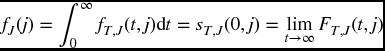
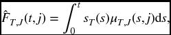
Suppose that T1, T2, …, Tm are failure times defined on the same sample space. In this chapter, we investigate the random variable
In other words, T is the time of the first failure to occur among the m different failure times that are possible. In particular, this will recast the material of Chapters 10 and 11 into a stochastic framework, and show that both joint-life theory and multiple-decrement theory are special cases of this general problem. In addition, it will provide more rigorous arguments for some of the results of those chapters that were obtained in an intuitive fashion. Finally it will deal with the important cases where the failure times need not be independent.
In the joint-life case, where we have a group of m lives numbered 1, 2, … , m, we can take Ti to be the future lifetime of the ith life, so that T is the failure time of the joint m-life status. In the multiple-decrement context, we can take Ti to be the time of failure from cause i in the associated single-decrement setting, so it is the failure time of the ith cause, assuming no other causes of failure are operating. Then, the random variable T is the time of failure in the multiple-decrement model. (In the machine analogy of Section 11.6, Ti would be the failure time of the ith part.)
17.2 Joint distributions
We wish to expand somewhat on our brief description for the case m = 2 given in Appendix A. Suppose that each Ti is continuous. There are various ways of describing the joint distribution. We can do so by the joint density function ![]() , or alternatively by the joint distribution function
, or alternatively by the joint distribution function
or by the joint survival function
To simplify the notation, we will often omit the subscripts and just write f, F or s when no confusion arises.
The reader is cautioned that s(t1, t2, …, tm) ≠ 1 − F(t1, t2, …, tm) when m > 1.
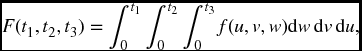
As in the one-dimensional case, we integrate to obtain the distribution or survival functions from the density function, and differentiate to go in the other direction. We must, however, use multiple integrals and partial derivatives. For example, with m = 3,
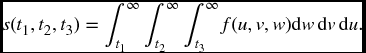
and similarly
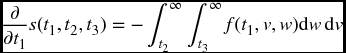
Now differentiate the latter expression with respect to t1. The fundamental theorem of calculus tells us to replace the variable u in the integrand with t1 and affix a minus sign since t1 is a lower limit. The integrand consists of the second two integrals. The result is
After two more iterations of the procedure, we have
Similarly, we can derive
Analogous expressions hold for general m, which appears as the exponent of − 1 in the first formula.
Note that the individual distributions are easily obtained from the the joint distribution or survival functions by
where the t is in the ith position, and ∞ indicates that you take limits.
17.3 The distribution of T
17.3.1 The general case
It is a simple matter to deduce the distribution of T from the joint distribution. Clearly, the minimum will take a value greater than t if and only if each Ti takes a value greater than t. Therefore,
(The reader should note that FT(t) ≠ F(t, t, …, t).)
17.3.2 The independent case
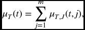
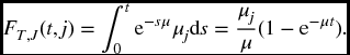
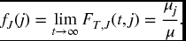
Let the density function, survival function, and hazard rate function of Ti be denoted respectively by fi, si, μi. Things become much easier to deal with when the random variables Ti are independent. We can then readily write down the relevant functions for T in terms of the corresponding functions for Ti. For example, from (17.2) we obtain
By taking logs and differentiating, we can find a similar relationship involving hazard functions.
We have already encountered a particular case of (17.4) in (10.10).
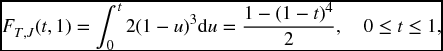
Example 17.1 Suppose that T1 and T2 are independent and both have the hazard function
Find the probability that the minimum value of these two random variables will be less than or equal to 1/2.
Solution. We note that sT(t) = (1 − t)4, for 0 ⩽ t < 1, either by first noting that, for i = 1, 2, si(t) = (1 − t)2 or by noting that μT(t) = 4/(1 − t). The desired probability is FT(1/2) = 1 − sT(1/2) = 15/16.
17.4 The joint distribution of (T, J)
17.4.1 The distribution function for (T, J)
Suppose that there is zero probability of the simultaneous occurrence of two or more failure times T1, T2, …, Tm. We can then define the random variable J as the index of the random variable giving the minimum. For an example with m = 3, suppose T1 = 7, T2 = 5, and T3 = 10. Then T would take the value 5, and J would take the value 2, since the minimum occurs for T2.
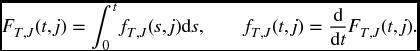
In many applications, we are interested in the joint distribution of T and J. This can be described in various ways. One method is by the joint distribution function,
This joint distribution has the somewhat unusual feature that the random variable T is normally continuous, while J is discrete. Therefore, unlike the usual notation for distribution functions, the second variable in FT, J(t, j) is not cumulative, but refers to one specific index.
We now consider the problem of deducing the joint distribution (T, J) from the joint distribution of T1, T2, …, Tm.
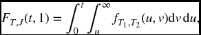
If we are given the joint density function, then FT, J(t, j) is calculated by integrating over a suitable region – see (A.17). Take m = 2. Then FT, J(t, 1) is the probability that T1 takes a value less than or equal to t, and that T2 takes any value that is greater than that taken by T1. This is given by the double integral
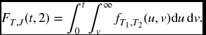
and similarly
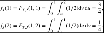
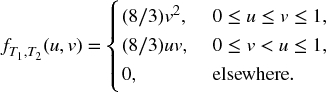
Example 17.2 The joint distribution of T1 and T2 is given by
Find FT, J(t, j) for j = 1, 2.
Solution.

By symmetry, we must have
Since Ti is bounded above by 1 for i = 1, 2, we necessarily have
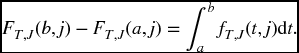
The sum of FT, J(t, 1) and FT, J(t, 2) must of course equal FT(t) = 1 − sT(t). It will be instructive for the reader to verify this by drawing a picture in the plane, showing that the union of the regions of integration in (17.5) and (17.17), and the region corresponding to sT(t), is the entire positive quadrant.
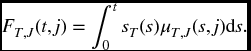
In the general case, we will need m-dimensional integrals to compute F(t, j) from the density function. However, if we already have the joint survival function, the computation can be simplified. To illustrate, consider the case with m = 3. Then, reasoning as above,
From (17.1) the inner two integrals can be written compactly as a partial derivative. We have
where
In the general case,
where
Example 17.3 Suppose that m = 2 and the joint survivor function is given by
Find FT, J(t, 1).
Solution. We could take two derivatives to calculate f(u, v) = 6(u − v)2, and apply (17.17). (This is in fact the same distribution as in Example 16.2.) Note, however, that (17.5) would just ‘undo’ the calculation of the second derivative by integrating. For this form of the distribution, it is easier to apply (17.17). On the given region
so
verifying the previous example.
17.4.2 Density and survival functions for (T, J)
We can also define the distribution of (T, J) by the joint density function fT, J(t, j). This is the function satisfying
The function f is interpreted in the normal way. Namely, for ‘small’ Δt, fT, J(t, j)Δt is approximately the probability that the first failure will be from cause j and that it will take place in the time interval from t to t + Δt. The precise statement, following from the first expression in (17.17), is that the probability that the first failure will be from cause j and will take place between time a and time b is given by
We define the joint survival function for (T, J) by thinking of survival as we did at the end of Section 11.2.2. Let
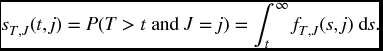
This is the probability that failure will occur after time t due to cause j.
Figure 17.1 shows a typical graph of f(t, j) for m = 2. Note that the mass is concentrated on parallel sheets. If we cut the jth sheet by the plane T = t, the area of the left portion will be F(t, j) and the area of the right portion will be s(t, j).
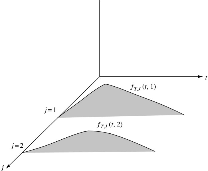
Figure 17.1 The graph of fT, J(t, j)
All functions pertaining to the random variable T alone are obtained by summing over all j, as we noted above for F in the case m = 2. That is,
17.4.3 The distribution of J
To obtain the distribution of J from the joint distribution, we compute the other marginal, which can be expressed in various ways. If fJ(j) denotes the probability that J = j, then
In Figure 17.1, fJ(j) is the area of the jth sheet. Note that FT, J(t, j) + sT, J(t, j) is not equal to 1, but rather to fJ(j).
Example 17.4 Take m = 2. If T1 is uniform on [0,1], T2 is uniform on [0,2], and T1 and T2 are independent, find the distribution of J.
Solution. The joint density function takes a constant value of 1/2 on the rectangle 0 ⩽ s ⩽ 1, 0 ⩽ t ⩽ 2, and is 0 elsewhere. The maximum value of T is the minimum of the respective maximums of the Ti, which in this case is 1. Therefore,
17.4.4 Hazard functions for (T, J)
Definition 17.1 The hazard function for (T, J) is given by

This is a conditional density. For small Δt, μT, J(t, j)Δt is approximately the probability that failure will occur first from cause j in the time interval from t to t + Δt, given that failure from any cause has not yet taken place before time t.
In the Chapter 11 multiple-decrement model for a life age x, μT, J(t, j) corresponds to μ(j)x(t).
Given the hazard rates, we can obtain the joint distribution of (T, J) by the same method as employed in Chapter 11. From (17.10) and the definition of μ(t, j),
and then, from (15.15),
We know that fT, J(s, j) = sT(s)μT, J(s, j) and, from the first expression in (17.17),
The last formula is easily explained intuitively. For the event in question to occur, there must be some point s, before t, for which failure from any cause has not yet occurred, and then failure will occur from the jth cause at time s Although (17.14) has this intuitive appeal, it is not necessarily useful for computing FT, J(t, j) as we may not know the joint hazard rates until we have already computed FT, J(t, j) and fT, J(t, j). It is, however, an important formula in the independent case to which we now turn.
17.4.5 The independent case
As in Section 17.2, we can simplify calculations when the Ti are independent, and deduce the distribution of (T, J) directly from the individual distributions of each Ti. Since s′j(t) = −sj(t)μj(t), (17.3) shows that
and then from (17.17),
Note, as a comparison to (17.14.), that (17.15) can be used directly to compute FT, J(t, j) in the independent case, when we know μi from the individual distributions. Moreover, differentiating and dividing by sT(t) verifies that in the independent case
for j = 1, 2, …m and all t for which sT(t) ⩾ 0, This provides the promised proof for the result stated in in formula (11.23).
The result is easily explained intuitively. Looking at the machine model of Section 11.6, for example, both quantities in (17.16) give a conditional density for failure of part j at time t. In the case of μT, J(t, j), the condition is that all parts have survived up to time t and in general this may give information regarding the failure time of part j. Suppose, for example, that the parts are connected so that part 2 cannot fail until part 1 does, and then it fails five seconds later. (The same idea in the multiple decrement model provided the simple counter-example of Exercise 11.15.) In the independent case, however, we obtain exactly the same information as if we told only that part j has survived up to time t, which is precisely the condition applicable to μj(t).
We have already encountered special cases of (17.17). One example is (10.10). The hazard rate μx(t) corresponds to μ1(t) which equals μT, J(t, 1) since we postulated independence. Another example is (11.11).
Example 17.5 Suppose that the Ti are independent and exponential with constant hazard μi. (a) Find FT, J(t, j). (b) Find fJ(j). (c) Show that T and J are independent.
Solution.
- Let μ = μ1 + μ2 + ⋅⋅⋅ + μm. Formula (17.4) shows that T is exponential with constant hazard μ, and, from (17.17),
-
- We just note that
The solution to (b) gives an important result that has many applications. It says that for independent exponential failure times, the probabilities of first failure are proportional to the hazard rates. This makes sense, since the higher the hazard rate, the lower the mean, which is the reciprocal of the hazard rate, and therefore more likelihood of occurring first.
Example 17.6 Take m = 2. Suppose T1 and T2 are independent, T1 is uniform on [0, a], and T2 is uniform on [0, b], where 0 < a ⩽ b. Find FT, J(t, 1) and FT, J(t, 2).
Solution. Since sT(t)μ1(t) = s2(t)s1(t)μ1(t) = s2(t)f1(t), we can write

Similarly,
Since failure must take place before time a, for any t ⩾ a,
As a check, note that FT, J(t, 1) + FT, J(t, 2) = F1(t) + F2(t) − F1(t)F2(t), which must be true, since for T to take a value less than t means that at least one of T1 and T2 takes a value less than t. Also note that the answer here could have been written down immediately, since the distributions satisfy the stochastic version of the condition given in (11.11), and therefore we can apply Method 2 of Chapter 11.
17.4.6 Nonidentifiability
We motivate the idea of this section by an example. First note that the joint distributions given in Examples 17.1 and 17.2 are easily seen to be different. One way is to note that T1 and T2 are not independent in the latter.
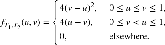
Example 17.7 Calculate FT, J(t, j) for the distribution given in Example 17.1
Solution. We could do this by (17.17), but it is easier to note that, by symmetry, FT, J(t, 1) = FT, J(t, 2) and the two must sum to FT(t) = 1 − sT(t). We can conclude directly from Example 17.1 that
and necessarily
Compare the above result with Example 17.2. The somewhat surprising conclusion is that two completely different distributions for (T1, T2) have led to exactly the same distribution for (T, J). This is known as the nonidentifiability problem and it has statistical implications. Suppose we want to make inferences about the joint distribution of the Ti by observing failure times. In many cases, all we can possibly observe is the joint distribution (T, J). An example is when the random variables represent the time of death from various causes. Once death occurs, we know the time and the cause, but no further observation of the subject is possible. Our example above shows that it is impossible to uniquely determine the joint distribution of the random variables that give rise to a given (T, J). We need additional information in order to obtain a unique solution. One instance when this occurs is in the independent case.
Theorem 17.1 Given any joint distribution for (T, J) there is a unique joint distribution of (T1, T2, …, Tm) such that the (Ti) are mutually independent and induce the given distribution of (T, J).
Proof. Uniqueness follows immediately, since, given independence, we know the joint distribution if we know the distribution of each Ti, and (17.16) implies that each Ti is necessarily a random variable with hazard function μT, J(t, i), which is determined uniquely from (T, J).
For the existence, given any joint distribution function F for (T, J), we let Ti be a random variable with hazard function μT, J(t, i). This collection of independent Ti in turn generates a joint distribution function ![]() . From (17.17),
. From (17.17),
which equals FT, J(t, j) as shown by (17.17).
![]()
To illustrate the use of this theorem, suppose you are told that
for i = 1, 2 and asked to identify the joint distribution of (T1, T2). You cannot do this without further information, for it could be either the joint distribution of Example 16.1 or that of Example 16.2, or indeed several other possibilities. However, if you are given the additional information that T1 and T2 are independent, then you know that it must be the distribution of Example 16.1.
17.4.7 Conditions for the independence of T and J
Another question of interest is to determine when T and J are independent. In Example 17.5, we saw that this occurred with constant hazard functions. We present here a more general criterion. Define the ratios
for all j, and all t, such that sT(t) > 0.
Theorem 17.2 K(t, j) = P(J = j|T = t). Therefore, T and J are independent if and only if K(t, j) is independent of t.
Proof. We have
So
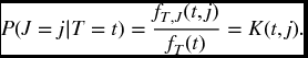
![]()
The condition of this theorem is sometimes expressed by saying that the hazards for the individual causes are fixed proportions of the total hazard.
17.5 Other problems
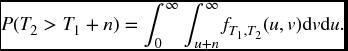
There are several other questions regarding the joint distribution of (T1, T2, …, Tm) that can be answered by similar techniques to those in Section 17.3. That is, we find a certain probability by integrating failure times over a suitable region of m-dimensional space. As an example, we illustrate the method for a problem analogous to Example 10.7 of Section 10.9. Take m = 2, and consider the probability that both causes of failure will occur within a specified duration of each other. That is, for some fixed n, we want the probability that (|T1 − T2| ⩽ n). It will normally be easier to compute this as
Each term is found by integrating the joint density function over a suitable region in the plane. For example,
Example 17.8 Find P(|T1 − T2| ⩽ n), when T1, T2 are independent, and both are exponential with hazard functions μ1 and μ2, respectively.
Solution. The integral above reduces to
so the final answer is
17.6 The common shock model
In many applications, we have a group of objects whose future lifetimes are generally independent, except that they are all subject to a common hazard, which will result in the failure of all, should it occur. In the case of human lives, this could be a natural disaster such as a hurricane. In the case of machine parts, it could be something like an electrical problem that affects all components at once. The presence of the common shock introduces dependence into what would otherwise be independent future lifetimes.
To model the general situation, we have m + 1 independent, continuous random variables, (T*1, T*2, …, T*m, Z), and for each i we let
The interpretation is that T*i is the time until failure of the ith object for reasons other than the common shock, and Z is the time until the common shock occurs. It follows then that Ti will be simply the time until failure of the ith object, since such failure will occur at either time T*i or time Z, whichever is earlier.
In the remainder of this section, we will confine ourselves to the case where m = 2. Quantities referring to T*i will have a superscript *.
We are interested in questions about the joint distribution (T1, T2), which involves dependent random variables. However, in many cases, we can answer these questions by considering the independent collection (T*1, T*2, Z). We will illustrate with several examples. A key fact to note is that
since both give the time of first failure.
Example 17.9 Find a formula for the probability that both objects will survive to time t.
Solution. This is just s*1(t)s*2(t)sZ(t).
Example 17.10 What is the probability that failure will occur as a result of the common shock?
Solution. This is just P(J = 3) in the joint distribution of (T, J), where J takes the values 1, 2, 3 and T is the minimum of T*1, T*2 and Z.
Example 17.11 What is the probability that the second failure will occur before time t?
Solution. We divide this up into two mutually exclusive cases. It will always occur if Z ⩽ t. If Z > t, we need both T*1 and T*2 less than or equal to t. The probability is
Other problems are not so straightforward and require special attention. The joint distribution of (T1, T2) is quite different from the typical two-dimensional continuous distribution. It still is continuous, but it has a mass of positive probability all concentrated on a single line, namely the diagonal, since the occurrence of the common shock will cause failure from both causes, leading to a failure point of the form (t, t). In determining the probability that (T1, T2) lies in some region A, we will in general have to break A up into three pieces, the part that is above the diagonal, the part that is below the diagonal, and the part that is on the diagonal.
We adopt the convention that the value of T1 is on the horizontal axis. For the part of the plane above the diagonal, {(u, v): u < v}, we use the joint density function
since the only way T1 can take a value u < v is if T*1 took the value u. In other words, failure from cause 1 at time u did not occur from the common shock, since if it did, then failure from cause 2 would also have occurred at time u and could not have occurred at the later date v.
Similarly, for the part of the positive quadrant below the diagonal, {(u, v): v < u}, we use the joint density function
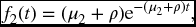
Since Ti = min (T*i, Z), the densities fi, i = 1, 2, are easily calculated as
Failure on the diagonal arises if and only if the occurrence of the common shock occurs before the other two causes. We use the one-dimensional density function,
and project the diagonal onto the line. That is, to find the probability that failure took place at a point (t, t), where a ⩽ t ⩽ b, we integrate this density from a to b.
Example 17.12 Suppose T*1, T*2, and Z are exponential with hazard functions μ1, μ2, and ρ, respectively. Consider the event that T1 and T2 are both less than or equal to n. This can be subdivided into three cases according as (a) T1 < T2, (b) T2 > T1, (c) T1 = T2. Find the probability of each case.
Solution.
- Note first that, from (17.17), we can calculate
so that, using the above-diagonal joint density, the required probability is
 which equals
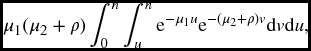
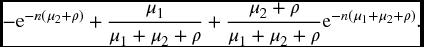
- Similarly, the required probability in this case is
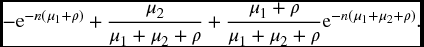
- The required probability is
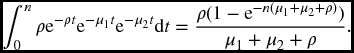
The sum of these three cases is
as we can verify from the general formula given in Example 16.12.
17.7 Copulas
This section, like the previous one, is concerned with situations where there is a lack of independence. We present a general method that is often used to deal with this. Attention is confined to the case m = 2.
A joint distribution (T1, T2) can be thought of as having two ingredients. One is the distributions of the two-component random variables, and the other is the way in which these are linked together. The latter can be described by a device known as a copula, which can then be applied to an arbitrary pair of individual distributions. The copula provides a means of dealing with these two ingredients separately. To elaborate, we start with the observation that whenever T1 and T2 are independent, we immediately recover the joint distribution from the individual distributions by the rule
We can then ask whether we can replace the multiplication on the right-hand-side of (17.18) by other transformations, and still obtain a joint distribution – that is, if I denotes the unit interval [0,1], whether we can find a function C from I × I to itself, so that we obtain a legitimate joint distribution by the rule
We need some restrictions on the function C. Take any point s in I. If T1 > s, so that ![]() , then, for all t,
, then, for all t, ![]() . The same holds for T2, leading to the condition that for all u, v in I,
. The same holds for T2, leading to the condition that for all u, v in I,
If T1 ⩽ s, so that ![]() , then for all t,
, then for all t, ![]() , leading to the condition that for all u, v in I,
, leading to the condition that for all u, v in I,
Another requirement stems from the fact that probabilities cannot be negative. For any sub-rectangle R⊆I × I, the probability that (T1, T2) lies in R is just the sum of the values of ![]() on the northeast and southwest corners, minus the sum of the values on the other two corners. Since this is nonnegative, it follows that
on the northeast and southwest corners, minus the sum of the values on the other two corners. Since this is nonnegative, it follows that
whenever u1 ⩽ u2 and v1 ⩽ v2.
These are the only conditions we need and we can now state the formal definition.
Definition 17.2 A copula is a function C from I × I to I satisfying (17.20)–(17.17).
It can be shown that if C is a copula, then (17.19) gives a valid joint probability distribution for any T1 and T2. Conversely (and harder to show), for any joint distribution (T1, T2) there is a copula C such that ![]() is given by (17.17).
is given by (17.17).
If T1 and T2 are both uniform distributions on I, then ![]() for i = 1, 2, and all u ∈ I, from which it follows that
for i = 1, 2, and all u ∈ I, from which it follows that
This shows that as an alternate definition, we can simply define a copula as a distribution function of a joint distribution involving two random variables that are uniform on I.
The following are three simple examples of copulas:
- C(u, v) = uv. This is just the copula for an independent distribution, as mentioned;
- C(u, v) = min (u, v);
- C(u, v) = max (u + v − 1, 0).
Copulas 2 and 3 are extreme in the sense that for any copula C and for all u, v, ∈I,
They are also extreme in the following sense. Consider all possible joint distributions for a given T1 and T2. In many cases, one is interested in the sum T1 + T2. For example, an insurer sells two insurance contracts and Ti denotes the claim on the ith policy, or a person buys two stocks and Ti is the value of the ith stock at some future date. We may want to compare all possible joint distributions as to their degree of risk. We will not go into the details of comparing joint distributions as to risk here. (In Section 22.4, we do introduce this idea for single variable distributions). However, it seems clear that risker possibilities arise when when large values of one random variable tend to go with large values of the other so there is a tendency for either both values to be large or both to be small. The less riskier possibilities arise when large values of one tend to go with small values of another, so there is a possibility for bad results in one case to be balanced by good results in the other. It can be shown, that under some natural risk comparing criteria, copula 2 will give the most risky joint distribution and copula 3 the least risky joint distribution. This point is illustrated further in Exercise 17.14.
We deal only briefly with problems of choosing a copula to model a given situation. In many cases, the modeler likes to choose a copula from a parametric family, and select the parameter to suit certain conditions. A popular choice for this is Frank’s family of copulas given by
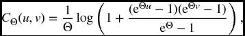
where Θ can be any nonzero real number. It can be shown, using L’Hôpital’s rule, that for all u, v, ∈I,
so that the smaller the parameter is in absolute value, the greater the extent of independence between the two random variables, with full independence occurring for Θ = 0.
An interesting feature which some copulas, but not all, have is that
It is straightforward to verify this property for copulas 1–3 above. It is true, but harder to verify, that this holds for Frank’s family. The significance of (17.23) is that
In other words, the same transformation rule can be applied to either distribution or survival functions.
Example 17.13 Suppose that Demoivre’s law holds with ω = 100. Consider two lives (60) and (70). Find the probability that both will be alive at the end of 10 years, assuming each of the three basic copulas given above, for the joint distribution of T(60) and T(70).
Solution. The individual survival probabilities are 3/4 and 2/3, so the survival of the joint-life status is in the respective cases:
- 1/2 as we known already from Chapter 10;
- min {3/4, 2/3} = 2/3. This copula applied to a joint-life status just means that the younger life will die at exactly the same time as the older;
- (3/4 + 2/3 − 1) = 5/12.
For a particular application of copulas, refer back to the nonidentifiability problem of Section 17.4.6. Instead of assuming independence, we might postulate a certain copula C and then ask for a joint distribution with the chosen copula that gives rise to the given distribution (T, J). In many cases this will be unique.
Notes and references
Nelsen (1999) is a good general source for additional material on copulas, including full derivations of the unproved results that we have given. Frees and Valdez (1998) discuss various actuarial applications of copulas. Carriérre (1994b) discusses the application of copulas to the nonidentifiability problem in multiple-decrement theory. For methods of comparing two-variable distributions for risk, see Shaked and Shantikumar (2007), Chapter 6.
Exercises
Type A exercises
- 17.1 A joint distribution is given by
Find FT, J(t, 1) and FT, J(t, 2).
- 17.2 A joint survival function is given by

Find FT, J(t, 1).
- 17.3 Suppose that T1 and T2 are independent with p.d.f.’s
- Find FT, J(t, 1) and FT, J(t, 2).
- Find the distribution of J.
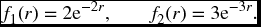
- 17.4 Suppose that T1 and T2 are independent. T1 has an exponential distribution with constant hazard rate μ. T2 is uniform on [0, a]. Find (a) FT, J(t, 2), (b) P(J = 2).
- 17.5 The failure times T1 and T2 are independent, and have respective hazard functions
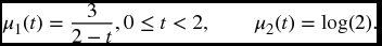
Find the probability that the minimum value of these two random variables will be less than or equal to 1.
- 17.6 A machine is subject to two independent causes of failure. The time of the first cause of failure is uniformly distributed on the interval [0, 4]. The time of the second cause of failure is uniformly distributed on the interval [0, 5]. Find the probability that: (a) the machine will fail from cause 1 before time 3; (b) the machine will eventually fail from cause 2.
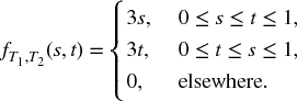
- 17.7 Two failure times T1 and T2 have a joint distribution given by the joint density function
Find: (a) FT, J(t, 1) and FT, J(t, 2); (b) the distribution of J; (c) μ(t, 1) and μ(t, 2).
- 17.8 Two failure times T1 and T2 have a joint distribution given by the joint density function
- Find FT, J(t, 1) and F − T, J(t, 2).
- Find the distribution of J.
- Suppose that
 and
and  are two independent variables whose joint distribution leads to the same distribution of (T, J) as you found in part (a). What are the hazard functions of
  and
and  ?
?
Type B exercises
-
17.9 For the joint distribution given in Example 17.2, find μ(t, j) and μj(t) for j = 1, 2. Show that these are not the same.
- 17.10 For the joint distribution given in Exercise 17.2, find μ(t, j) and μj(t) for j = 1, 2. Show that these are not the same.
- 17.11 Consider independent failure times T1 and T2 where the hazard rate of T1 is α/(1 − t), 0 ⩽ t < 1, and the hazard rate of T2 is β/(1 − t), 0 ⩽ t < 1. Answer the following in terms of α and β.
- Find FT, J(t, 1).
- Find P(J = 2).
- An insurance contract provides for a benefit at the moment of the first failure, provided that this is due to ‘cause 1’ (i.e. provided that T1 < T2). The amount of the benefit for failure at time t is (1 − t)e0.1t. The force of interest δ is a constant 0.10. Find the expected present value of the benefits.
- 17.12 Two lives age (x) and (y) are subject to the common shock model. T*(x) has a constant hazard rate of 0.06, T*(y) has a constant hazard rate of 0.04, and Z has a constant hazard rate of 0.02. The force of interest is a constant 0.05.
- Calculate
 and write it as a sum of three terms, namely, the expected present value of benefits when: (i) (x) dies at a time strictly before the death of (y); (ii) (x) dies at time strictly after the death of (y); (iii) (x) dies as result of the common shock.
 - Calculate
 .
.
- Calculate
- 17.13 You are given a common shock model (T*1, T2*, Z) where T*1 has the survival function s(t) = 1 − 0.1t, T*2 has a constant hazard function of 0.04, and Z has a constant hazard function of 0.02. Find the probabilities that (a) T1 < T2, (b) T2 < T1, (c) T1 = T2.
- 17.14 Suppose that T1 and T2 each take the values 0 with probability 1/2, and 1 with probability 1/2. Calculate the probability function for the joint distribution of (T1, T2) under each of the following copulas: (a) C(u, v) = min (u, v), (b) C(u, v) = max (u + v − 1, 0), (c) C(u, v) = uv, (d) Frank’s copula with values of θ = 0.01, 50, −50. What happens when θ approaches ∞ or − ∞?
- 17.15 A joint life insurance on (x) and (y) has death benefits which are constant over each year. Assume that either copulas 2 or 3 of Section 17.7 apply to the joint distribution of T(x) and T(y). Show that unlike the independent case, the term R in equation (10.15) is equal to 0.