22
Risk assessment
22.1 Introduction
The previous chapter was largely devoted to computing or approximating the distribution of aggregate claims for the losses on an insurance portfolio. The next problem that arises is to effectively use this information to assess and manage the risk associated with the insurer’s commitment to pay these losses. Similarly, a consumer is interested in assessing the extent to which their risk is transferred by the purchase of insurance. We alluded to this theme somewhat in Part II of the book but we now wish to investigate some of the issues in more detail. Our concentration will be on a more general basic question that has application in many areas. Given two or more uncertain alternatives, how do we compare or measure the amount of risk associated with each? This is a large topic and we confine ourselves here to a survey of some of the main ideas. It is important in what follows to distinguish between two cases. The quantities in question may involve losses in which case less is better, or gains, in which case more is better. We could conventionally fix one or the other, by introducing minus signs, but that complicates the notation, so we rely on the context to clarify what is intended. We start in the next section by talking about gains.
22.2 Utility theory
One method which may seem natural for deciding between two random payouts is to compare the expected amounts that you will receive. However, this does not always give reasonable answers and does not always conform to choices that rational people actually make, as the following example indicates. Imagine that you are offered the following two risky alternatives. In alternative 1, you gain 200 with probability 0.99, or lose 10 000 with probability 0.01. In alternative 2, you gain 200 with probability 0.5 or lose 10 with probability 0.5. Alternative 1 has an expectation of 98, which is greater than 95, the expectation of alternative 2. However, nearly everybody would reject alternative 1 with the possibility, although small, of a very large loss. Expectation does not take into account the amount of the risk involved.
Perhaps the most famous example of the drawbacks inherent in using the expected value as a decision tool is the St. Petersburg Paradox, formulated by Daniel Bernouli in the eighteenth century. His explanation marked the beginning of the concept of utility theory. A game consists of tossing a coin until a head appears, with a payout of 2n if this occurs on the nth toss. The expectation of the amount to be won is then ∑∞n = 12n(1/2n) = ∞, but it is not reasonable to expect that someone would pay an arbitrarily large amount to play this game. Bernouli introduced the idea that one should not consider the actual amounts paid but rather the ‘satisfaction’ or ‘utility’ that comes with possessing a certain level of wealth. In other words, he postulated that each individual has a so-called utility function u, where u(x) denotes the utility that the person derives from having x units of wealth. It is expected that u is an increasing function of x, as more wealth gives additional utility, but that the rate of increase diminishes with increasing x. A person who is already a multimillionaire will derive little satisfaction from an additional 1 unit of wealth, while somebody who is destitute would welcome it greatly. In mathematical terms, it is expected that for most people u is a concave function. (We give a precise definition in Section 22.3.) If u is differentiable, the above features simply mean that the first derivative of u is nonnegative and the second derivative is nonpositive. A typical example of such a function is log x which was chosen by Bernouli in his explanation of the St. Petersburg Paradox. He argued that one should consider the expected utility rather than the expected value of the actual amounts, and indeed ∑∞n = 1log (2n)(1/2n) is finite.
People with concave utility functions are called risk-averse, since they prefer certainty to uncertainty, and therefore derive utility from insuring, as the following example illustrates.
Example 22.1 People are faced with a potential loss of 100, which will occur with probability 0.1. Their goal is to maximize the expected utility of their resulting wealth. How large a single premium P would they pay to insure against such a loss if their utility function is given by u(x) = log (x), and their initial wealth is (a) 1000? (b) 500?
Solution. In part (a), if they do insure, they will have utility of u(1000 − P) = log (1000 − P), which is certain; while if they do not insure, they will have an expected utility of 0.9u(1000) + 0.1u(900) = log [(1000)0.9(900)0.1]. Equating the resulting expected utility, the largest P they would pay is given by
which is solved to give P = 10.48. So such individuals would be willing to pay more than the expected loss of 10 in order to acquire the utility they derive from the extra security.
In part (b), the equation changes to 500 − P = 5000.94000.1 which is solved to give P = 11.03. The premium is higher, reflecting the fact that people with the lower wealth are less prepared to suffer a loss and will pay more for insurance. This indicates the important fact that in general one must take into account initial wealth and not just the particular transaction when comparing alternatives as to expected utility. (See Exercise 22.1 for an exception to this statement.)
Economists use many other choices of utility functions in their desire to model people’s preferences. One of the most popular choices is the family of so-called power utility functions. This is a parametrized family, which includes the log function, and is defined by
for some parameter γ ≥ 0. It is clear that the first two derivatives have the property stated above.
Readers should not be dismayed by the fact that uγ(x) can take negative values, for as long as we use these for comparative purposes there is no difficulty. Indeed, if we replace any utility function u by the function au + b, where a and b are constants with a > 0, it follows from the linearity of expectation that we will always obtain the same results when comparing two alternatives as to expected utility.
From this point of view we could have described the above family by the functions x1 − γ for γ < 1 or − x1 − γ for γ > 1. However, an advantage of the given form is that we can define the value at γ = 1 by taking a limit. Applying L’Hopitals rule, we get
As γ increases, individuals become more risk-averse, as indicated by the fact that they will pay more to reduce risk. For example if we redo part (a) of Example 22.1 with γ = 2, we get the equation
which is solved to give P = 10.99, an amount greater than the premium of 10.48 for γ = 1.
Note that γ0(x) = x − 1 which indicates there is no risk aversion and comparison is done simply by expected values. A person with such a utility function is the risk-neutral individual described in Section 20.5.
People with a convex (defined in Section 22.3) utility function would be termed risk-seekers as such people will pay to gamble, even at unfavourable odds, (typical of the usual casino). The following example illustrates the effect of such a utility function.
Example 22.2 People with an initial wealth of 10 are offered a chance to play a game in which they win either 2 or 0, each with probability 1/2. If their utility function is given by the convex function u(x) = x2, what is the most they will pay to play this game.
Solution. Let P be the amount paid to play the game. We equate the expected utility of not playing versus playing which gives the equation
Solving, P = 1.0501, which is more than the expected winnings of 1.
The examples of this section should provide further clarification of the difference between insurance and gambling that we alluded to in Section 1.1. In the next section, we provide some more precise definitions and mathematical verification of our conclusions.
22.3 Convex and concave functions: Jensen’s inequality
22.3.1 Basic definitions
Definition 22.1 A real-valued function g defined on an interval I of the real line is said to be convex if for all x and y in I and 0 ≤ α ≤ 1:
Geometrically, this says that a line segment joining any two points of the graph of g will lie above the graph.
A feature of convex functions that is often used is the increasing slope condition which states that for three points x < y < z in I,
To derive (22.2) note that
so that
Now multiply this equation by (z − x)/(z − y)(y − x) = (y − x)− 1 + (z − y)− 1 to get
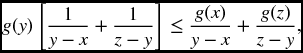
and rearrange to get (22.22).
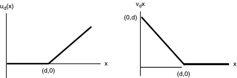
Figure 22.1 Graphs of ud(x) and vd(x)
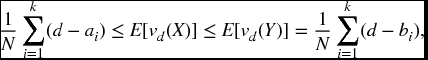
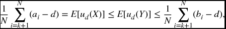
Many readers will be familiar with the result from basic calculus that for twice differentiable functions, convexity is characterized by the fact the second derivative is nonnegative. The advantage of the general definition above is that we can apply it to the functions that have points of nondifferentiability, such as the two families of functions (using the notation of Section 21.10.1):
whose graphs are shown in Figure 22.1. Any piecewise linear function (one whose graph consists of a finite number of straight line segments) can be written as a linear combination of the ud′s and vd′s. In view of the increasing slope condition, a convex piecewise linear function can be written as a linear combination of these with positive coefficients. For example, the function defined on the real line by
can be written as v0 + u0 + 2u2.
Definition 22.2 A function defined on an interval I of the real line is said to be concave if the inequality reverses in (22.1) and therefore also in (22.22).
For concave functions, straight line segments between any two points of the graph are now above the graph. For twice differentiable functions the second derivative is nonpositive. Clearly, a function g is concave if and only if − g is convex.
22.3.2 Jensen’s inequality
We introduce a basic inequality for risk assessment. To motivate, imagine that you are presented with a bag with two numbered balls. You draw one at random and receive the square of the number. If both the balls had number 5, you get 25 for sure. What if they were numbered 4 and 6, which average 5? You now get an expected payoff of 0.5(36 + 16) = 26 > 25, so the randomness has produced an extra expected return over the certain case. We can see exactly why this happens by writing
and
The key to this result then is the fact that ( − 1)2 = 1. When you average, the middle terms cancel but the squared term is the same for the positive and negative deviations, giving the extra amount. This calculation shows that you will get the same conclusion for any two numbered balls. What about for three balls? Say you have numbers 1, 2, 6 which average 3. The average of the squares is 13 2/3 which is greater than 32. Indeed, the principle involved holds in great generality since the inequality
where μ = E(X), shows that for any random variable X, the expectation of X2 must be greater than or equal to the square of the expectation of X.
What happens for other functions other than the square? For the square root function, the inequality goes the other way. If you have two balls numbered 16 and 4 with an average of 10, the average of the square roots is 3 which is less than ![]() . It turns out that we get the extra return with any convex function, and therefore a reduced return from the average with any concave function. The formal statement is as follows.
. It turns out that we get the extra return with any convex function, and therefore a reduced return from the average with any concave function. The formal statement is as follows.
Theorem 22.1 (Jensen’s inequality) For any convex function g,
Proof. We will give the proof in the case where g has a continuous second derivative. The idea is that by our remarks above, it is true for any polynomial of degree two which has a positive coefficient of x2. Taylor’s theorem from basic calculus tells us that g can be approximated by such a polynomial. Precisely, if E(X) = μ, then
for some point ξ between μ and x. Of course we do not know ξ but we do not need it, since if g is convex, then g′′ is nonnegative, and the left-hand side is greater than or equal to the sum of the first two terms. Taking expectations,
completing the proof.
![]()
Jensen’s inequality obviously reverses for a concave function, as seen by applying the statement above to the function − g. This shows that in general we have the conclusions shown by the particular examples of the last section. That is, as we would expect, risk-averse individuals prefer certainty to risk. Such individuals with initial wealth w who pay E(X) to insure against a loss X will have resulting utility of u(w − E(X)) which is greater than E[u(w − X)]. Therefore, they are willing to pay somewhat more than the expected value of the benefits. This makes the business of insurance economically feasible, since as we indicated in previous chapters, the insurer must necessarily charge more than the expected value of the loss in the form of loadings for expenses, profits and risk.
22.4 A general comparison method
In this section, we consider the general problem of comparing two random variables as to their degree of risk. There are many ways of defining such an order relationship. We will concentrate on one of the early definitions, introduced in Rothschild and Stiglitz (1970) which ties in with the utility theory concept. For simplification, we concentrate on the equal mean case.
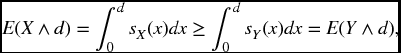
Definition 22.3 For nonnegative random variables X and Y with E(X) = E(Y), we say that X is less risky than Y, if for all d,
For example, if our random variables represent losses, then the net premium for deductible insurance that covers losses above a certain amount is always less for the less risky option. It is clear that this relation does not depend on the actual random variables but only on their distribution.
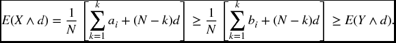
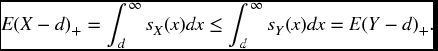
In view of the equal mean hypothesis, formula (21.11) shows that an equivalent formulation is that for all d ≥ 0,
We can apply the above inequalities to the functions introduced in the previous section. The result is that if X is less risky than Y, then for all d ≥ 0,
and therefore, for any piecewise linear convex function g,
since the positive coefficients, when we express g as a linear combination of the ud and vd for various values of d, will preserve the order. Now given an arbitrary convex function, we can approximate it by a piecewise linear one as follows. Choose a large number of points on the graph and join them with straight line segments. The increasing slope condition shows that this approximating function will be convex. The more points that we choose, the better the approximation will be. By standard approximation techniques in analysis it follows that (22.6) holds for all convex functions (we do not give the exact details here), and of course the reverse inequality holds for concave functions. We are therefore led to the conclusion that if risk-averse individuals have to choose between two distributions of their final wealth, both of the same mean, they will choose the less risky one according to our definition, in order to maximize expected utility. This justifies the definition given by Rothschild–Stiglitz as one which truly captures the concept of riskiness.
It is not always easy to decide whether one random variable is less risky than another, but there are certain instances when we can verify this. It is assumed in the following two theorems that E(X) = E(Y).
Theorem 22.2 Suppose that X takes the values a1 ≤ a2 ≤ … ≤ aN − 1 ≤ aN each with probability 1/N and Y takes the values b1 ≤ b2… ≤ bN − 1 ≤ bN each with probability 1/N. Then X will be less risky than Y if and only if
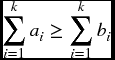
for 1 ≤ k ≤ N.
Proof. Suppose the condition holds. Then, given d where ak ≤ d < ak + 1, we have
The last inequality follows from the fact that bi∧d is less than or equal to both bi and d for all i.
Conversely, suppose X is less risky than Y. Fix any index k < N, and let d = max {ak, bk}. Invoking (22.22), we see that, if d = bk, then
while if d = ak, then
In either case, condition (22.7) follows in view of the fact that the equal mean hypothesis implies that ∑Ni = 1ai = ∑Ni = 1bi.
![]()
Remark Since repetition of values is allowed, the above theorem can be applied to all finite discrete distributions where the probabilities are rational numbers.
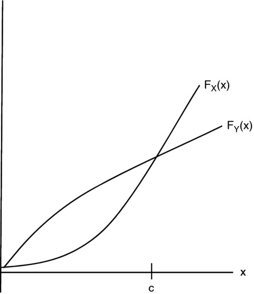
Figure 22.2 The cut condition: X is less risky than Y
Here is another condition which applies to all distributions. We can view this geometrically as saying that if two distribution functions intersect at one point, then the steeper curve gives the the less risky distribution (see Figure 22.2).
Theorem 22.3 (The cut condition) Suppose that for some point c,
Then X is less risky than Y.
Proof. We use formulas (21.10) and (21.21), and note that the stated inequalities in the premise reverse with s in place of F. If d < c,
while if d > c,
By continuity of the function g(d) = E(X − d)+, we must obtain the same result at d = c. In all cases we have by definition that X is less risky than Y.
![]()
Remark The definition of being less risky and the cut condition apply equally well to random variables that take negative values. The complication in the proof is that formula (21.12) no longer holds as given and a suitable modification is required. We leave this to the interested reader.
Readers should be aware that our ordering in this case is what mathematicians call a partial order, meaning that certain pairs are incomparable. Given a choice of X and Y, it may happen that some risk -averse people would prefer a final wealth of X and others would prefer Y, so neither is less risky than the other according to our definition. Here is a typical example.
The random variable X, representing a gain, takes the value 1 with probability 0.1 and 10 with probability 0.9, while an alternative Y takes the value 2 with probability 0.9 and 73 with probability 0.1. Both have a mean of 9.1. One might expect a risk averter to choose X, ensuring themselves of a return of 10 in most cases, rather than gamble on the higher return which most of the time will lead to a return of only 2. However, by Theorem 22.2, since 1 < 2, while 11 > 4, they are incomparable. This happens since there could be someone so risk averse that they could not tolerate even the small chance of a return of only 1. Indeed, consider the following scenario. Suppose individuals absolutely need 2 units of wealth or something dreadful will happen to them. They might well want to ensure that this terrible fate cannot occur by choosing Y.
Of course, when we are able to make a comparison, the conclusion is that much stronger. As a typical example we will prove a well-known result on optimal choices of insurance, which was proved in Arrow (1963).
The idea is as follows. Suppose that individuals want to ensure against a loss by paying some fixed premium, which is however insufficient to provide for full coverage, and so they must arrange for partial reimbursement.
Let X denote a random loss (assumed to be nonnegative) and P denote the premium they want to pay. They must choose some I(X), a function of X, which will be the amount paid to them when loss occurs. We make the natural assumption that 0 ≤ I(X) ≤ X, so that the amount paid cannot be negative and cannot exceed the amount of the loss. We assume that to provide the coverage, the insurer charges a premium that is a function π of E[I(X)]. Any of the modifications discussed in Section 21.10.1, as well as others, could be used. As an example, suppose the insurer charges a 20% loading above the expected value of the loss and E(X) = 100, while P = 60. The insured then is only going to pay one-half of the premium necessary for full coverage. One way of doing so is to choose I(X) = 0.5X so whatever the loss is, the insured will receive one-half of this amount as reimbursement. Another alternative is to set a maximum on the amount paid, and of course there are many other possibilities. Which choice is best?
Theorem 22.4 Given the assumptions above, any risk-averse individual should choose deductible insurance, in order to maximize the utility of resulting wealth.
Proof. Suppose the individuals start with an initial wealth of a. Their resulting wealth after paying the premium, incurring the loss and being reimbursed, will be
In particular let I0(X) = (X − d)+, where d is chosen to satisfy π[E(I0(X))] = P, and let W0 be the resulting wealth for this case. Apply the cut condition with c = a − P − d. Since W0 is never less than c, then ![]() , for any t < c. Consider now the case when t > c. If W0 > t, then X − I0(X) < d, so the loss must have been under the deductible. From our assumption that reimbursement cannot exceed the loss, we must have I(X) ≤ d, showing that W ≥ W0 > t. It follows that
, for any t < c. Consider now the case when t > c. If W0 > t, then X − I0(X) < d, so the loss must have been under the deductible. From our assumption that reimbursement cannot exceed the loss, we must have I(X) ≤ d, showing that W ≥ W0 > t. It follows that ![]() completing the proof.
completing the proof.
![]()
The conclusion seems intuitively clear since deductible insurance avoids large catastrophic losses, which should appeal to the risk averter.
Remark We leave to the interested reader the following extension of the above problem. The individual truly interested in maximizing utility would normally not specify the desired premium in advance, but would let that vary as well. The problem now is not only to choose the form of insurance but also to choose P, which will be a function of the initial wealth.
22.5 Risk measures for capital adequacy
22.5.1 The general notion of a risk measure
In some cases we want to do more than just compare the riskiness of two random variables. We actually want to assign a number that in some sense quantifies or measures the risk, and of course that will then allow us to compare two or in fact any number of random variables. A function that assigns a number to a certain class of random variables is known appropriately enough as a risk measure. We already encountered this concept in Section 15.6.4. Assigning a premium to a random variable representing the benefits paid on an insurance contract is a form of risk measure.
Another important use of this concept is to arrive at the amount of capital that should be held to cover possible losses. Now we have already introduced the concept of a reserve to provide for future obligations. Recall, however, from Section 15.5 that the reserve is the expected amount that one needs, and it is provided for by the excess premiums that are collected in early years. The reserve is not intended to provide for unexpected large losses. If these occur, the company will have to draw on surplus in order to maintain the required reserves, and the question is, how much capital should be on hand for this purpose. This idea is not just confined to insurance. Measures for this purpose are extensively used by the banking industry. The method that has been almost universally adopted by banks is a quantile-based approach, which we have already discussed in Section 15.7. For present purposes, we now introduce some more precise definitions and terminologies.
22.5.2 Value-at-risk
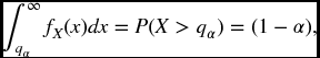
Suppose we have a random variable X and a number α between 0 and 1. A number x, such that FX(x) = α, is known as an α-quantile of X. (An alternate terminology is to multiply α by 100 and speak of a percentile. For example, a 0.7 quantile can be referred to as 70th percentile.) The 0.5 quantile is commonly referred to as the median of the distribution.
When the values of FX vary continuously from 0 to 1 over some interval, then F− 1X(α) is the unique α-quantile. We will denote this number by qα. In other cases there might not exist any such number, or there might exist infinitely many. The former arises when the value of FX jumps at a point x from a number less than α to one more than α. In that case we take qα to be the point of the jump. Such a point will of course be equal to qβ for several different values of β. The case of infinitely many values arises when for some x, FX(x) = α, but X does not take any values in some open interval with a left endpoint of x. For example, if FX(3) = 0.7 and the probability of X taking a value in the interval (3,3.1) is zero, then FX(x) is also equal to 0.7 for any x in the interval (3, 3.1). For our purposes we will want to single out the smallest such number. We can then cover all cases by the following.
Definition 22.4
When X represents losses, or an amount that to be paid out, qα can be viewed as a type of risk measure, with higher values signifying more risk. The percentile premium was a risk measure of this type. In the banking industry, this risk measure has been termed value-at-risk and abbreviated as VaR. (The capital R at the end distinguishes it from the common notation for ‘variance’. It is pronounced to rhyme with ‘far’.) VaR is expressed with a certain time horizon and a confidence level α, often taken to be a number reasonably close to 1 such as 0.95 or 0.99. For example, to say that a certain investment portfolio has a 1 day VaR of 100 000 means that 100 000 will be sufficient to ensure that the losses over the next day will be covered most of the time where ‘most’ is measured by the specified confidence level.
22.5.3 Tail value-at-risk
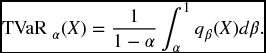
There are problems with VaR, as we have already noted in connection with percentile premiums. It does not take into account how bad the losses can be when they exceed the chosen quantile. In the above example, if there were a possibility of a loss of several million, which occurred with probability less than (1 − α), we still would have a VaR of only 100 000. The possibility of this large loss would be completely ignored in our risk measure. For this, and other reasons, many people have advocated a modification of VaR known as tail value-at-risk (abbreviated as TailVar or just TVar). The same measure is also known as conditional tail expectation, abbreviated as CTE or sometimes TCE.
For a given confidence level α, TVaRα is essentially defined as the expected loss given that the loss is in excess of the quantile qα. Problems can arise in interpreting the words ‘in excess of’. Do these words mean ‘strictly greater than’ or ‘greater than or equal to’? The distinction is irrelevant for continuous distributions, but in the discrete case they can give different results, and, strangely enough, neither may be the one that you want. For example, suppose that somebody tosses a penny and a dime and you must pay them 1 for each head. Set α = 0.5. The median loss is 1, and TVaR0.5 should be the expected value in the worst one-half of the distribution. There are four possibilities of equal probability giving respective losses of 0, 1, 1, 2, so we want to select the two worst cases. Of course there is a tie, but a logical way to handle this is to arbitrarily pick any one of the two coins, say the penny, and we then say that the the two worst outcomes will be when both coins come up heads, or the penny only comes up heads. With this reasoning TVaR0.5 should be 0.5( 1+2) = 1.5. However, the expected loss, given that the loss is strictly greater than 1, will be 2, and the expected loss, given that the loss is greater than or equal to 1, will be 4/3. Readers are cautioned that there are examples in the literature where the ‘strictly greater than’ or ‘greater than equal to’ methods are used in defining TVaR and similar risk measures. However, both of these can lead to inconsistencies. See, for example, Exercise 22.6. These are avoided by the definition below, which follows from the idea presented in this simple example.
For a continuous distribution we define our desired risk measure by
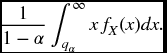
Now by definition
so we can add and subtract qα on the right-hand side to get the following.
Definition 22.5

The above formula is the best form of the definition to use as it applies to any distribution, not just a continuous one.
As a check, we verify that it gives the results we expect in the discrete case. (In particular we retrieve the answer of 1.5 obtained in the coin-flip example.) We calculate TVaR for the particular type of discrete random variables considered in Theorem 22.2. For a definite example, let N = 10 and suppose that our confidence level α = 7/10. Then VaR0.7(X) clearly equals a7 which will cover the loss whenever the outcome is ai, i ≤ 7 which occurs 7/10 of the time. What about TVaR0.7?
From Definition 22.5, this is just
as we would expect. In general, if α = r/10 for an integer r, then VaRα(X) = r/10 and TVarRα(X) = (ar + 1 + ⋅⋅⋅ + a10)/(10 − r).
Things are a bit more complicated when for some integer r, (r − 1)/10 < α < r/10. Suppose in the above example that α = 13/20 which is between 6/10 and 7/10. We still get VaR α(X) = a7, but now (1 − α)− 1 = 20/7, so Equation (22.9) yields

The general formula is as follows. If α = (r − p)/N where r is an integer and 0 < p < 1, then
where β = p(N − r + 1)/(N − r + p). We leave this for the reader to verify. To actually compute TVaR in this discrete case, it is usually more efficient to use Definition 22.5 directly, but (22.11) is useful for demonstrating properties of TVaR, as we will illustrate later.
Many people believe that a risk measure H used for premiums or capital adequacy should be subadditive. Namely they want that
After all, if we have to set aside H(X) of capital to provide for a risk X and a further H(Y) of capital to provide for a risk Y, then it is reasonable to suppose that we will not need more than this sum if we take on both risks. (This viewpoint is not completely universal and some argue that such activities as mergers can produce inefficiencies and cause other problems that actually increase the total risk.) We already saw in Example 15.6 that a quantile risk measure does not satisfy subadditivity, and this has been a major criticism levelled against the use of VaR. On the other hand, TVaR is subadditive. A complete general proof is somewhat advanced and we will confine attention here to show this for the discrete random variables that we introduced above, where the proof is straightforward and clearly indicates the reason for the result.
Suppose we have a sample space {ω1, ω2, …, ωN} each with probability 1/N and X takes the value ai on ωi. where ai ≤ aj for i ≤ j. Suppose that the random variable Y takes the value bi on ωi.
Assume first that bi ≤ bj for i < j. The random variables X and Y in the this case are said to be comonotonic. Precisely this means that for two sample points, if X takes a higher value on one of them, then Y will also take a higher value on that point. In other words they move together. (This concept can been generalized to arbitrary distributions and plays a major role in risk assessment.) Take α = r/N. In this case, the N − r highest values of X + Y will be of the form ar + 1 + br + 1, ar + 2 + br + 2, …, aN + bN and from (22.10) it is clear that
This is a reasonable conclusion. In the case of comonotonicity, we cannot hope to have a high value in one random variable offset by a low value in the other. There is no diversification effect and combining the random variables does not lead to a reduction in the total risk measure. Now suppose that we remove the comonotonicity by rearranging the b′s. Obviously, the N − r highest values of ai + bi cannot get any larger than what we had in the previous case, where we included the N − r highest values of both the a’s and b’s. The left side of (22.12) must stay the same or decrease, and this implies the required subadditivity when α is as given. Now, we can invoke (22.11) to see that it holds for any α.
Besides subadditivity, there are other desirable features of risk measures that are satisfied by TVaR but not VaR. See, for example, Exercise 18.13.
Following are two examples which compute TVaR for familiar distributions.
Example 22.3 Compute TVaR for a normal distribution.
Solution. In the case of a standard normal Z, the density function satisfies xfZ(x) = −f′Z(x). From (22.8) and the fundamental theorem of calculus,
where Φ is the c.d.f. of Z.
It is not difficult to show that for any X and constants a and b, with b > 0, TVaRα(a + bX) = a + bTVaRα(X). Therefore, if X is a normal distribution with mean μ and variance σ2, we have
Example 22.4 Compute TVaR for a exponential distribution.
Solution. First we note that if X ∼ Exp(λ) then qα = s− 1X(1 − α) = −log (1 − α)/λ. From Equation (21.21), Example 21.7, and the fact that sX(qα) = 1 − α by definition, it follows that E(x − qα)+ = (1 − α)/λ. Now from Definition 22.5,
We conclude this section by providing an equivalent formulation of TVaR for continuous distributions, which serves to illustrate further how the information in the tail which is ignored in VaR gets incorporated into TVaR. In the integral (22.22), make the substitution β = FX(x). We have x = qβ(X), dβ = fX(x)dx so that
This says that we can view TVaRα as an average of all the VaRs at confidence levels greater than α.
22.5.4 Distortion risk measures
Here is another equivalent formulation of TVaR. For any α in the interval (0, 1), let gα denote the function on [0, 1] defined by
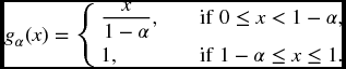
Then from (21.10) and Definition (22.22),
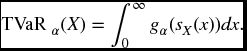
A whole family of other risk measures arises if, in the above formula, we replace gα by any continuous function g that increases from 0 to 1. These are known as distortion risk measures. Note that when g(x) = x we just get E(X) as the risk measure. The concept has been termed by some as a sort of dual approach to that of taking expected utility. In the latter case we distort the amounts paid by converting them into utilities. In this case we distort the probabilities. Smaller values of the survival function, corresponding to right tail events, are increased in value, in an attempt to reflect the risk. It can be shown that any concave function g will give a subadditive risk measure.
Notes and references
The order relation we introduced in Section 22.4 is sometimes referred to as the convex order in view of (22.22). The same definition with the equal mean hypothesis eliminated is known as the stop loss order.
More detailed information on ordering risks can be found in Kass et al. (2008). This same reference contains additional material on utility theory.
Readers particularly interested is risk measures may consult Artzner et al. (1999), which deals with ‘coherency’, a much discussed topic in recent years.
Exercises
- 22.1 For any α > 0 define a utility function by uα(x) = −e− αx. (This is known as exponential utility.)
- Show that a person with this utility function is risk averse.
- Show that when comparing risky alternatives to maximize utility by using uα, the result is independent of initial wealth.
- In Example (22.1) let Pα denote the premium that would be paid when using uα as a utility function. Calculate P0.02, P0.01 and limα → 0Pα. What happens to risk adversity as α decreases?
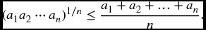
- 22.2 Use Jensen’s inequality to prove the well-known arithmetic–geometric mean inequality. For positive numbers ai, 1 ≤ i ≤ n,
Hint: Take an appropriate distribution and let g(x) = log x.
- 22.3 Consider the two random variables X ∼ exp(2) and Y ∼ exp(3) + 1/6. Compare as to riskiness according to the definition given in Section 22.4. That is, is X less risky than Y, or is Y less risky than X or are they incomparable?
- 22.4 Compare the following three distributions as to riskiness:
- X takes the value 1 with probability 1/6, 2 with probability 1/3, 3 with probability 1/3 and 6 with probability 1/6.
- Y takes the value 2 with probability 1/2, 3 with probability 1/3 and 5 with probability 1/6.
- Z takes the value 1 with probability 1/6, 2 with probability 1/6, 3 with probability 1/3, and 4 with probability 1/3.
- 22.5
- Show that X less risky than Y implies that the variance of X is less than the variance of Y.
- Show that the converse is true in the normal case. That is, for normal random variables X and Y with the same mean, the one with the smaller variance will be less risky.
- 22.6
- On a sample space of three points, ω1, ω2, ω3, a random variable X takes the values (1,1,3) and a random variable Y takes the values (1,2,3). Consider the risk measure H(Z) = E[Z|Z > q0.3]. Show that despite the fact that Y takes values at all sample points that are greater than or equal to those of X, we have H(X) > H(Y).
- Find an example that works as the above only now with H(Z) = E[Z|Z ≥ qα] for some α.
- 22.7 Suppose X ∼ Gamma(2, 3). For a certain value of α, VaR(X) = 4. Find TVaR(X).
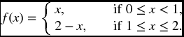
- 22.8 The random variable X has a density function given by
Find VaRα(X) and TVARα(X) for α = (a) 1/2, (b) 31/32.
- 22.9 Find VaRα(X) and TVaRα(X) when X is uniform on [0,N].
- 22.10 A random variable X takes the values 1 with probability 4/7, 3 with probability 2/7 and 6 with probability 1/7. Find VaR0.8(X) and TVaR0.8(X).
- 22.11 A random variable takes on the values x1, x2, …, x40, each with probability 1/40. If TVaR0.85(X) = 100 and TVaR 0.875(X) = 150, find TVaR0.86(X).
- 22.12 On a sample space consisting of four points that have equal probability, the random variables X and Y take, respectively, the values (1,2,3,4) and ( 4,1,2,3). Consider the distortion risk measure H given by the function g(x) = x1/2.
- Calculate H(X), H(Y), H(X + Y) and verify that the subadditivity holds.
- Suppose that Z is an other random variable on this space taking the values (a, b, c, d), where a ≤ b ≤ c ≤ d. Verify that H(X + Z) = H(X) + H(Z).
- 22.13 Suppose that X and Y both take N values each with probability 1/N, E(X) = E(Y) and that X is less risky than Y. Show that TVaRα(X) ≤ TVaRα(Y), but it is not necessarily true that VaRα(X) ≤ VaRα(Y).
- 22.14
- If X is a distribution such that TVaR α(X) – VaR α(X) is independent of α, what must this constant difference be?
- Show that an exponential distribution has this property.
- 22.15 (This question refers back to material introduced in Part I of the book.) Assume that interest rates are positive, that is, the investment discount function v(t) is decreasing with t.
- Show that
 is a concave function of t.
 - Use Jensen’s inequality to show that

- Now assume constant interest. A 1-unit whole life policy on (x) has premiums payable continuously at the annual rate of P. Show that
That is, the expected amount of premiums accumulated at death by a policyholder is greater than or equal to the benefit payment at that time.
- Explain the inequality in (c) by general reasoning. (You may want to refer to Section 8.4.3.)
- Show that the inequalities in (b) and (c) are equalities at 0 interest.
- Show that