
19
Multi-state models
19.1 Introduction
Multi-state models are an attempt to look at a variety of life insurance and annuity contracts in a unified manner, by making use of Markov processes. As motivation, take an individual now age x and consider a two-state Markov chain, where the person is in state 0 (alive) or state 1 (deceased) at any time. Life insurance contracts provide benefits upon transfer from state 0 to state 1, while life annuity contracts provide benefits as long as the process remains in state 0.
More generally, consider a multiple-decrement model for (x) with m causes of failure. We can consider a chain with m + 1 states. State 0 means that (x) has not succumbed to any cause and is often referred to as the active state. State j refers to having succumbed first to cause j. The insurance benefits discussed in Chapter 11 can be viewed as payments upon transfer from state 0 to other states.
For still another example, consider a joint-life contract issued to (x) and (y). We can now take a chain with four states as illustrated in Figure 19.1. The arrows indicate that there are possible transitions from state 0 into state 1 or state 2, occasioned by the death of (y) or (x) respectively, and then further transitions from state 1 or state 2 into state 3 when the second death occurs. The dotted line, showing a transition directly from state 0 to state 3, would not be present in our original model, but would be there if we wanted to consider a common shock model as discussed in Section 17.6. A joint life insurance can be considered as two contracts, one paying benefits upon transfer from state 0 to state 1, and the other paying benefits upon transfer from state 0 to state 2. A general two-life annuity can be considered as three separate contracts, where the ith contract, i = 0, 1, 2, pays benefits provided the process is in state i. This can be generalized to contracts involving n lives where we will have 2n states.

Figure 19.1 A two life multi-state model
We can of course imagine more general patterns of transition. We may wish to investigate a more enriched multiple-decrement model where individuals can transfer between states several times. A disabled person might recover and re-enter the main group of lives. In our original model we ignored what happened to a life once it left the group for any cause, but we may wish to model the fact that someone leaving for a cause other than death will subsequently die. There are many examples of insurance and annuity benefits applicable to this general case. When disability is one of the decrements, we may have a contract that pays benefits when a person becomes disabled, and then further benefits when a disabled person dies, and possibly additional payments that continue during disability. Indeed, a common provision in many life insurance policies is a disability premium waiver clause, which mean the person does not have to pay premiums during the time they are disabled. We view this as an annuity providing payments during a state of disability, which cease when there is a transfer back to an active state. These are only some of the possibilities, and we invite the reader to think of additional applications.
In this chapter, we will investigate the general multi-state model. We first discuss the discrete-time model, where transitions between states can occur only at integer times. Following that we deal with the more complicated continuous-time model, where we allow for transitions at arbitrary times.
19.2 The discrete-time model
19.2.1 Non-stationary Markov Chains
The transitions in multi-state models are normally age-dependent. To handle this, we need to extend the concepts and notation that we introduced in Section 18.4.1 so that they apply to the non-stationary case.
For a non-stationary Markov Chain, in place of the single transition matrix P, we need for each nonnegative integer n, a matrix Pn whose ijth entry is pij(n, n + 1)
The main quantities of interest are the probabilities pij(k, n) of being in state j at time n conditional upon being in state i at time k. In deriving (18.18), we do not need the fact that the matrices are the same, and the argument given is easily adapted to show that
which reduces to (18.5) in the stationary case. Equation (18.6) now takes the form
For example, in our simple life-death chain the transition matrices are given by
In the multiple decrement example, the matrix Pn will be similar to that above, except the first row will be (p(τ)x + n, qx + n(1), q(2)x + n, …, qx + n(m)), and each other row will have 1 on the main diagonal and 0s elsewhere.
We leave is as an exercise for the reader to write down the matrix Pn in the joint two life case.
We now introduce a multi-state model which is not covered by our previous cases of multiple lives or multiple-decrement theory, and to which we will refer to frequently in the rest of the chapter. It allows for a two-way transition between certain states, which is really where the generality of the multi-state model is the most helpful. This is the chain as depicted in Figure 19.2 where a life can be healthy or unhealthy, but we now allow for recovery from the unhealthy state.
There are various applications, The unhealthy state could refer to being disabled, or sick, or a number of other possibilities for a state which we wish to distinguish somehow from the main group of lives, but which can transfer back to the main group.
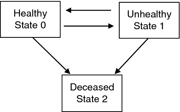
Figure 19.2 The healthy-unhealthy-deceased model
Example 19.1 Consider the model of Figure 19.2 and suppose that transition matrices for times 0, 1, 2 are given as follows;
What is the probability that a person who is healthy at time 0 will be unhealthy at time 2 and deceased at time 3?
Solution.
Using formula (19.19), the required probability equals
19.2.2 Discrete-time multi-state insurances
To model the general contract of this type, we will take a Markov chain with states numbered from 0 to N. Suppose the process begins in state a at time 0. Fix any two states i and j, and consider a contract which pays a benefit of bk at time k + 1, provided a transfer from state i to state j occurs between time k and time k + 1. That is, the process was in state i at time k and state j at time k + 1.
Notation If we have several different transfer benefits we will distinguish by writing bk as ![]() . In general, for quantities like benefits, premiums, reserves and expenses, we will let superscripts refer to states, and maintain our previous usage of subscripts to refer to time. This differs from our convention for probabilities where we use subscripts to refer to states, and write times in brackets.
. In general, for quantities like benefits, premiums, reserves and expenses, we will let superscripts refer to states, and maintain our previous usage of subscripts to refer to time. This differs from our convention for probabilities where we use subscripts to refer to states, and write times in brackets.
A convenient method of discussing multi-state benefits in the context of the stochastic model is to make use of indicator random variables. For each nonnegative integer k, let Ik be the random variable that takes the values of 0 or 1 respectively, accordingly as a transfer from i to j has not or has occurred between time k and k + 1. The present value of the benefits on the contract is given by
Since
the actuarial present value is
We again have our familiar pattern with a sum of three-termed factors. In fact, we can consider each summand as a four-termed factor where the probability of receiving a payment is itself the product of two factors, the probability of transition to state i by time k and the probability of transition from state i to state j in the next period.
Example 19.2 Consider the chain given in Example 19.1. A 3-year contract written on a healthy life provides for benefits at the end of the year of death. The death benefit is 3 if the person dies while healthy and 2 if the person dies while unhealthy. If interest is a constant 5%, find the actuarial present value.
Solution. We can view this as two separate contracts, one paying 3 for transfer from state 0 to state 2, and the second paying 2 for transfer from state 1 to state 2. We use the matrices in Example 19.1 and formula (19.19). For the first contract,
so that
For the second contract,
so that
Therefore, the total APV is 1.2912.
Example 19.3 Take the same chain as in the previous example. Consider a contract that pays 1 at the end of any year of transfer from being healthy to being unhealthy, provided this occurs within the next 3 years. Find the expected value and variance of the benefits.
Solution. We now have
so that
The variance calculation can not be done conveniently by adapting a version of formula (15.15). The situation here is different from the multiple decrement model where benefits are paid upon transition to an absorbing state. In this case, there can be benefits paid at more than one time. We must instead use the approach taken in the current payment formula for annuity variances. Note however that the covariance calculations will be more complicated than that given by (15.15). Letting Ik take the value 1 if transfer from the healthy state to the unhealthy state occurs between time k and k + 1, we have
while
which is the probability of becoming unhealthy, recovering, and then becoming unhealthy again, thereby being paid at both time 1 and time 3. We can then calculate the covariances as
leading to the calculation of the variance as
Suppose we wished to modify the contract of the previous example so that it paid off only on the first occurrence of becoming unhealthy. In our simple example, this could be done readily enough by changing the probability of a benefit payment at time 3 to 0.105, subtracting 0.006, which we have calculated above as the probability of the second occurrence. To handle the problem in general, we need a more systematic approach. Consider a contract paying benefits upon the first transition from a state i0 to a state j0. A method that works here ( as well for many other problems ) is to add additional states.
The easiest way is to add a single new absorbing state z, and all transfers from state i0 to state j0 are redirected to z, and the contract is modified to pay upon a transfer from i0 to z. To state this precisely, let p* denote probabilities in the augmented chain. To simplify the notation, fix a time n and write pij and p*ij for pij(n, n + 1) and p*ij(n, n + 1) respectively. Then p* is the same as p except that
There is a more involved method which has the advantage that it preserves relationships between other states that might be needed in more complex problems. This is to add N + 1 new states i*, i = 0, …, N, where state i* can be considered as a sort of ‘clone’ of state i. Transitions between un-starred states are as before except that transitions from i0 to j0 are directed to j*0 in place of j0. Except for that, there are no transitions between the two types of states, starred and un-starred. Transitions between starred states are as given by the corresponding transitions between their clones. In this case, ![]() and for all ordered pairs (i, j) not equal to (i0, j0),
and for all ordered pairs (i, j) not equal to (i0, j0),
For example, if our original matrix for a two state model is given by
and we take i0 = 0, j0 = 1, the the matrix of the augmented chain, using the order 0, 1, 0*, 1* is
In addition to this, the provisions of the insurance are modified to pay upon a transfer from state i0 to state j*0. After the first occurrence of such an event, there can never be a return to state i0, so subsequent occurrences are ruled out.
Remark Solving multi-state problems with large matrices can involve a great deal of calculation. There are a number of computing packages that can assist with this. One convenient example is the MMULT function of Excel®.
19.2.3 Multi-state annuities
We now look at annuity contracts associated with a chain. Suppose again that the individual begins in state a at time 0. For a fixed state i, we can consider a contract that pays ck at time k provided the person is in state i at that time. Let Ik now be the indicator random variable that takes the value of 1 or 0 according as the process is or is not in state i at time k. Then the present value of the benefits is the random variable
from which we calculate immediately

To derive variances, we calculate for all m < n
From this, we calculate the covariances and then proceed as in Example 19.3.
Example 19.4 Consider again the chain given in Example 19.1. A contract on a healthy life provides for four yearly payments beginning at time 0. The amount of the payment is 1 if the person is healthy, or 2 if the person is unhealthy. If interest is a constant 5%, find the actuarial present value.
Solution. We view this as two separate annuities. Contract 1 is for state 1 and contract 2 is for state 2. In addition to the matrix P0P1 calculated in Example 19.1, we need
The APV of contract 1 is
and that of contract 2 is
giving a total APV of 3.6150.
Example 19.5 Suppose the contract in Example 19.2 is to be purchased by three level annual premiums of π, which are payable only if the person is healthy. Calculate π.
Solution. Equating values of premiums and benefits,
which gives π = 0.6449.
There are other types of annuity contracts that can be handled by the trick of adding states. Suppose for example, a contract provides periodic annuity benefits starting when the process enters state i0 (or starting at time 0 if the process begins in state i0), but which stop completely when the process leaves state i0, even if there is a subsequent return. The easiest approach here is to add an absorbing state z and all transitions from state i0 to other states are directed to state z, ensuring the process never returns to i0. If we want to preserve information about other transitions, the method is to add a clone for each state as we did in the insurance case. Transitions from state i0 to any state j ≠ i0 are redirected to the clone j*, also ensuring that the process will never return to state i0.
19.3 The continuous-time model
In a realistic situation, transitions between states need not occur at discrete intervals, but can happen at any point of time, and the benefits payable upon transition from one state to the another will be paid at the moment of transition. To model this situation, we need to consider continuous-time Markov processes. We still keep a finite number of states, but let time vary continuously. The definition parallels that which we make in Section 18.2, only we must consider all possible points of time. (We will follow the notational usage introduced in Section 18.5 of writing the time variable in brackets.)
Definition 19.1 A continuous-time Markov process is a stochastic process X(t): 0 ⩽ t < ∞, where each X(t) is discrete, with the property that given any sequence of times, 0 ⩽ t0 < t1 < ⋅⋅⋅ < tn < tn + 1, and any sequence (x0, x1, x2…xn, xn + 1) where xi is a value of X(ti) we have
As before, for times s ⩽ t and any two states i, j we let
which is the probability of reaching state j at time t when starting in state i at time s.
19.3.1 Forces of transition
With the continuous time framework, we are able to define analogues of the force of mortality in our original life-death model, and the forces of decrement in the multiple-decrement model. As we have seen in earlier examples, the process is often specified by giving these forces, and then the central problem is to use these to calculate the desired probabilities.
Definition 19.2 We define the force of transition from state i to state j at time t as follows. If i ≠ j
while
Note that μii is always nonpostive, which may seem a bit strange at first, but it is easily explained if we consider, for example, the multiple-decrement case where state 0 refers to an active life. The negativity of μ00 reflects the action of the other forces of decrement, which cause transfer out of state 0.
An important fact is the following.
Theorem 19.1
Proof. Fix any i and t. Refer to the little o notation introduced in Section 18.3. From the definitions above, for all states j and h > 0,
and
Summing over all j gives
Subtract 1 from each side, divide by h and take a limit as h approaches 0 to establish the conclusion.
![]()
We now want to relate the forces of transition to the transition probabilities. This is much more complicated in our general setting than in the simple cases we looked at previously.
Theorem 19.2 (Kolmogorov forward equations) For any states i, j and times s < t

Proof. We start by deriving the discrete version of the above formula. Following the reasoning used in Equation (18.18), we can deduce that for states i, j times s < t and h > 0
reflecting the fact that in order to reach state j from state i in the time interval s, t + h we must first reach some state k by time t and then go from state k to state j in the next h time units. The system of equations given by (19.10) is known as the Chapman-Kolmogorov equations.
Substituting from (19.7) and (19.8) into the second factor of the summand,
Subtracting pij(s, t) from both sides, dividing by h and taking a limit gives (19.19).
![]()
We can give an intuitive explanation of (19.9) paralleling that given in the discrete case. View each side as a type of density function for reaching state j at time t when starting from state i at time s. The right side reflects the fact that in order to accomplish this, we must first reach some state k at time t and then at that instant of time, transfer from state k to state j (or in the case that k = j, not transfer back into some other state).
We view the statement of the theorem as a system of differential equations in the variable t for a fixed value of s. The word ‘forward’ arises since our transition is moving forward in time. There is a related system, the corresponding backwards equations, which will be developed in Exercise 19.6.
There will normally be many solutions to a system of differential equations of this type. There will however often be a unique solution if we specify appropriate initial conditions. In our context, these conditions are the obvious requirements that for all t,
We have of course encountered versions of the Kolmogorov equations before. Take s = 0. The simplest case with N = 1 gives Equation (8.8). In the multiple decrement model, the Kolmogorov equations produce Equation (11.11). These statements may not be completely obvious since the notation is somewhat different. It will be instructive for the reader to verify these claims.
There is a nice matrix formulation of (19.19). Fixing s, t we let P denote the transition matrix for the time interval (s, t). This is the matrix with an entry in the ith row and jth column of pij(s, t), as we had in the discrete case. We also have a corresponding matrix M in which the entry in the ith row and jth column is μij(t). M is often referred to as the intensity matrix. We let P′ denote the matrix in which each entry is the partial derivative with respect to t of the corresponding entry in P. The Kolmogorov forward equations together with the initial conditions can then be expressed as
and
The following is a simple but useful consequence of the forward equations. It generalizes a result from our life-death model, when we have a state, such as that of being alive, which cannot be entered from any other state. That is, for all j ≠ i and s < t, we have pji(s, t) = 0. We will refer to such a state as being anti-absorbing.
In the following theorem, we adopt a formally weaker hypothesis involving forces rather than probabilities, which by the second statement turns out to be equivalent.
Theorem 19.3 Let i be a state such that μji(t) = 0 for all j ≠ i, and all t. Then, for s < t,
and
Proof. From Theorem 19.2 we get
a familiar differential equation which we first encountered in (8.15) and which is easily solved to give
for some function K(s) independent of t, Since pii(s, s) = 1, and pji(s, s) = 0 for j ≠ i, we must have K(s) = 1 if j = i or 0 if j ≠ i and the conclusion follows.
![]()
Another quantity of interest is the so-called sojourn probability for a state. We define
Note that the sojourn probability will in general differ from pii(s, t), as the corresponding event requires the process to remain in state i for an entire interval of time, rather than just at the endpoints. The two probabilities will however be the same for an anti-absorbing state.
Since sojourn probabilities are featured prominently in the next section, we will attempt to find a way to evaluate them. Let
This is the probability that starting in state i at time s, the process is back in state i at time t, having left state i sometime during the interval. Let
Now we employ once again the technique of adding states. Given a process and a state i, we add a single new state i* which is a clone of state i. Transitions out of state i* follow the same pattern as transitions out of state i, while transitions that originally came into state i will be diverted to the cloned state i*. Now to say that the new process is in state i at a time s and also at a later time t means that it must have stayed there throughout as it cannot re-enter. In addition, the forces of transition out of state i remain the same in both processes. So we have that
We do have to consider the quantity ![]() . Now
. Now
since the new process will move from state i to state i* precisely when the original process moves from state i back to state i having left state i at some point. From Definition 19.2,
Applying Theorem 19.3 to state i in the new process then leads to the formula
This formula does not however allow one to calculate the term on the left exactly since νi also involves sojourn probabilities. All we can say without further assumptions is that
Suppose, however, that we have a process such that, for all states i and t, h > 0
This assumption says that it is highly unlikely that in a small time interval there is a move out of a state and back into it. It is the same idea that underlies a Poisson process as discussed in Section 18.3, where it was highly unlikely to have two occurrences of an event in a small time interval. When this assumption holds, we have that vi(t) = 0 for all t and we can now state the following theorem.
Theorem 19.4 For a process satisfying (19.19),
Remark We can view the first statement in Theorem 19.3 as the special case of Theorem 19.4, when qi is actually equal to 0.
An alternative direct proof of Theorem 19.4 is outlined in Exercise 19.18.
To summarize our conclusions in this section we have shown that given the forces of transition, we can in theory, solve a system of differential equations to arrive at the required probabilities that we are interested in for our applications. However, in practice, the solution can be difficult or impossible to obtain exactly. In the following subsections we look at various possibilities for obtaining or approximating the probabilities from the forces.
19.3.2 Path-by-path analysis
Assume then that we are given μij(t) for all i, j and t, and we want to determine the probability that starting in state i at any time s, we will be in state j at time t. What we can do in a relatively straightforward manner is the following. Given any path going from state i to state j, we can derive a formula for the probability that starting in state i at time s, the process will be in state j at time t, having following the prescribed path exactly. Precisely, we are given a path π which is a sequence of states, i0, i1, …, iM where i0 = i and iM = j. We then want the probability that the process will make a transition from state i to i1 followed by a transition from i1 to i2, followed by a transition from i2 to i3 and so on, continuing in such a fashion, without visiting any other states, and finally reaching state j at or before time t, and remaining in state j until time t. Let us denote such a probability by pπi, j(s, t). These can be calculated by integration, using only the forces and sojourn probabilities. So assuming that (19.14) holds, we have reduced the problem to one of evaluating integrals.
To illustrate, consider the simplest possible case of a path of length 1, that is π = (i, j). Then arguing much the same as we did in the single life and multiple decrement models we can write

The above formula parallels formula (11.13) except that in that case all non-active states are absorbing, so one cannot get out of them, which means that the third factor in the integrand does not appear as it is equal to 1. To recap, the formula above shows that in order to go from i to j along the one-step path, three events have to occur. First, the process must remain in state i until some time r between time s and time t. This event has probability ![]() . It cannot first go to another state and return, since that would constitute a different path from the given one. Secondly, there must be a transition to state j at time r. We can think of the probability of this as being μi, j(r)dr. Finally, the process must remain in state j from time r to time t. It cannot leave state j and return as this would similarly constitute a different path. We get the required probability by integrating the product of these probabilities over all times r between s and t.
. It cannot first go to another state and return, since that would constitute a different path from the given one. Secondly, there must be a transition to state j at time r. We can think of the probability of this as being μi, j(r)dr. Finally, the process must remain in state j from time r to time t. It cannot leave state j and return as this would similarly constitute a different path. We get the required probability by integrating the product of these probabilities over all times r between s and t.
As the path length increases the formula gets more complicated. Consider a two-step path, π = (i, k, j). Now we need a double integral. The formula is
This looks extremely complex, but it simply records what are now five steps to meet the required conditions. The process must remain in state i until some time r1, then transfer to state k, then remain in state k until some time r2, then transfer to state j, and then finally remain in state j until time t.
A similar calculation that arises for a given path Π, is to find the probability that starting in state i at time s, the process will transfer to state j before time t having followed precisely the prescribed path. We get the same multiple integral as described above, except the final sojourn probability is omitted, since the process need only enter, but not necessarily remain in the final state on the path. Of course, when the final state is absorbing, the two problems are identical.
Example 19.6 Consider a heathy-unhealthy-deceased model as introduced in Figure 19.2. The forces of transition are constant with μ01 = 2, μ02 = 1, μ10 = 1, μ12 = 3. Find the probability that a healthy life will become unhealthy, and then die without recovering before time 1.
Solution. We have μ00 = −3, μ11 = −4. The path in question is π = (0, 1, 2) and the required probability is

The double integral evaluates to
In general, a path of length n will require an n-dimensional integral with an integrand consisting of 2n + 1 factors, so this can quickly become computationally infeasible. Aside from that there is another difficulty. Usually, what we really want is pij(s, t). In some cases this might be obtained by adding up pπi, j(s, t) for all possible paths π from i to j. However, even in the simplest of models, there could well be an infinite number of such paths and this procedure will not work. This will normally occur whenever there is a positive probability of two-way transitions, as in the healthy-unhealthy-deceased model where healthy people can recover. A person could go from a healthy state to the deceased state, by getting sick and dying, or getting sick, then recovering, then getting sick again and dying, or recovering twice before death, or any of a number of infinite possibilities. We need other approaches to calculating transition probabilities, which we discuss in the next two subsections.
19.3.3 Numerical approximation
There are various ways to find a numerical approximation to the solution of the Kolmogorov equations. We will describe one approach that is fairly simple to implement. It is similar to Euler’s method, described in Section 8.9, for Thiele’s equation. For a fixed time s, the goal is to approximate the probabilities pij(s, t). Pick a small interval of time h, and change our unit of time, so that each original time unit is now 1/h units. (So, for example, if our original time unit was a year, and h = 1/12, this changes the time unit to months.). We then essentially define a discrete time multi-state model, which will in generally be nonstationary. We will define one step transition probabilities for this model by simply looking at formulas (19.7) and (19.19), which formed the basis of the Kolmogorov equations, only omitting the o(h) terms in each case. Since these terms becomes very small as h does, we can hope that for small enough h, we obtain a good approximation. We also switch the origin of time so that the original time s is now time 0 and the original time s + mh for an integer m is now time m. We then take our approximating discrete non-stationary Markov chain to be that in which the transition probabilities, denoted by ![]() , are given by
, are given by
We then obtain transition matrices ![]() which have for an (i, j)th entry, the quantity
which have for an (i, j)th entry, the quantity ![]()
Another way of looking at this is that we simply get the matrix ![]() by taking the intensity matrix M(s + mh), multiplying all non-diagonal entries by h and adjusting the diagonal entries so that the rows add to 1.
by taking the intensity matrix M(s + mh), multiplying all non-diagonal entries by h and adjusting the diagonal entries so that the rows add to 1.
When t = s + mh for some integer m we can then obtain approximations by
Example 19.7 In a chain with three states, you are given that
Find an approximation to p01(1, 2) using the method described above with h = 1/3.
Solution. We have
so that

and similarly
Then the approximation to p01(1, 2) is the entry in row 0 and column 1 of ![]() , which is 0.15131.
, which is 0.15131.
19.3.4 Stationary continuous time processes
One case where we can make some progress in solving the Kolmogorov equations directly is that of a stationary process as defined in Chapter 18. We then have that each μij(t) is a constant, denoted by μij. Moreover, the process will be determined by the quantities pij(t) = pij(0, t) since the stationary condition implies that pij(s, t) = pij(t − s).
As an example, we can write down completely the solution for the general two-state stationary process. Suppose the intensity matrix is
Let ρ(t) = e− t(μ + ν). Then the transition matrix P(t), which has the entry of pij(t) in the ith row and jth column, is given by

We can verify that P satisfies equations (19.11) and ( 19.12) by direct calculation, noting that dρ(t)/dt) = −(μ + ν)ρ(t), and that ρ(0) = 1.
For the general stationary process, solutions to P′ = PM can be generated from eigenvectors of M. These are non-zero vectors ![]() for which
for which
for some constant λ known as an eigenvalue of M. (The left hand side above is a matrix multiplication in which we view a as a 1 × N + 1 matrix. According to the convention we have used for the transition probabilities, the vector appears on the left.) To obtain eigenvectors, we first find the eigenvalues as those constants for which the determinant of (λI − M) = 0. This involves solving a polynomial equation in λ. We can then solve for the resulting eigenvectors. Examples will follow.
Note now that given any such eigenvector a and any fixed i, the matrix P that has all zero entries except for an ith row of (a0eλt, a1eλt…aNeλt) is a solution to P′ = PM. This follows since the ijth entry of PM will be λajeλt which is the derivative of the corresponding entry in ![]() .
.
Note next that given any finite number of solutions to P′ = PM, the linearity implies that any linear combination of these solutions will also be a solution. We therefore seek a linear combination that will satisfy the initial conditions. This can always be done in the case that we can find N linearly independent eigenvectors. We illustrate with a simple example.
Example 19.8 For the data as given in Example 19.6, find the probabilities of the following events.
(a) A life now disabled will be active at time 0.5.
(b) A life now active will be deceased at time 1.
Solution. The intensity matrix is
We can see immediately that 0 is an eigenvalue with an eigenvector of (0, 0, 1).
We can also note that since the rows of P add up to 1, the rows of ![]() add to 0, and the last row of P is (0, 0, 1), it is sufficient to solve the reduced system
add to 0, and the last row of P is (0, 0, 1), it is sufficient to solve the reduced system ![]() in which the superscript r indicates a matrix with the row N and column N removed. So we can consider eigenvectors of
in which the superscript r indicates a matrix with the row N and column N removed. So we can consider eigenvectors of
The determinant of λI − Mr is λ2 + 7λ + 10 giving eigenvalues of −5 and −2. Solving, we find respective eigenvectors of (1, −2) and (1, 1). (Note that eigenvectors are not unique as they can be multiplied by any non-zero constant.).
To satisfy the initial conditions, we want the first row of Pr to be the particular linear combination of the vectors a = e− 5t(1, −2) and b = e− 2t(1, 1) which gives the vector (1, 0) when t = 0. We solve this to get a first row vector of (1/3)a + (2/3)b. For the second row, we want a linear combination that gives the vector (0,1) when t = 0. We solve this to get a second row vector equal to ( − 1/3)a + (1/3)b. Transition probabilities are then given by
The answers to the particular questions asked are
- p10(0, 0.5) = 0.0953.
- 1 − p00(0, 1) − p01(0, 1) = 0.8218.
(The answer to part (b) is of course larger than that of Example 19.6 since here we allow for an arbitrary number of recoveries from being sick, as well as death from a healthy state.
19.3.5 Some methods for non-stationary processes
The above procedure can also be used solve the problem of determining probabilities from the forces, when these are ‘piecewise constant’. We can find transition matrices for each time interval on which the forces are constant, and then use the discrete time technique. The following simple example illustrates the procedure. It involves only two time intervals but the method can easily be extended.
Example 19.9 For a two-state model, we have forces of transition given by
Find the probability that the process will be in state 1 at time 2.5 given that it is is state 0 at time 0.
Solution.
From the matrix (19.19), we have
Substituting, the required probability is 0.39446.
One method for handling a perfectly general chain is to approximate it by a piecewise continuous one, and then use the method outlined above. To do so, one can choose a small time unit, and approximate the forces of transition by replacing them with those that are constant on each time interval, possibly using the midpoint value.
19.3.6 Extension of the common shock model
As mentioned in the introduction, multiple life theory, multiple decrement theory, or the more general model discussed in Chapter 17 can all be looked at in a multi-state framework. In the standard cases where failure times are independent, this does not normally provide any advantage over the conventional treatments that we have described previously. The multi-state approach, however, can be useful in modelling certain types of dependence. As an illustration, we will revisit the common shock model of Section 17.5 and discuss some possible refinements. We confine the analysis to the case of two types of failure, the first with failure time equal to min (T*1, Z) and the second with failure time equal to min (T*2, Z). Failure for the two types is dependent due to the common shock but there will be additional sources of dependence when T*1 and T*2 are themselves not independent. An example of this is the ‘broken-heart’ syndrome mentioned in Section 10.2 where one type of failure can hasten failure of the other type.
We consider a multi-state model with four states, as given in Figure 19.1, but adapted to cover general failure times. State 0 means that neither type of failure has occurred, state 1 means that only the second cause of failure has occurred, state 2 means that only the first type of failure has occurred, and state 3 means that both types of failure have occurred. (The states 1 and 2 then are labelled by the number of the surviving type.) Let μi(t) denote the hazard function for T*i, and ρ(t) denote the hazard function for Z.
Suppose that forces of failure are of the form.
for some functions ε1(t) and ε2(t). When these are 0, we have precisely the common shock model. In this more general setting, we use εi(t) to build in some dependence between T*1 and T*2 by letting the distributions change after the first failure. The ‘broken-heart syndrome’ would call for positive values of εi(t). On the other hand, there may be cases where we assume that the prospects for failure type i improves after the first failure, and we would reflect this with a negative εi(t).
Probabilities in this model can all be calculated by the procedure of Section 19.3.2 since there are at most three paths between any two states. Moreover, since no state can be re-entered once the process leaves it, we can use Theorem 19.4 for the sojourn probabilities.
For the following examples we assume that all forces are constant.
Example 19.10 Calculate the probability that at time n, the first type of failure will have occurred but not the second.
Solution. From Theorem 19.1,
We want

The integral is easily evaluated to give
As a check, suppose that ε1 = ε2 = ρ = 0, so we simply have two independent exponential failure times. The answer reduces to
which is just the probability that the first type of failure occurred before time n multiplied by the probability that the second type did not occur before time n.
Example 19.11 Find the probability that the second cause of failure occurs before time n and after the first cause of failure.
Solution. If Π is the path (0,2,3) we want,
(a special case of formula (19.17) in the next section.) Substituting from (19.16) and integrating, the answer is
When ε2 = 0 we recover the answer of Example 17.12 (a).
19.3.7 Insurance and annuity applications in continuous time
Consider an insurance contract that provides for two fixed states j and k, payments at the moment of transfer whenever a transfer occurs from state j to state k. The amount paid for a transfer at time t will be bt (denoted by b(jk)t if we wish to distinguish between several transfer benefits). Suppose the process is in state i at time 0. Then the actuarial present value parallels the result we saw in the multiple decrement case and is given by
If benefits are to be paid on only the first transfer from state j to state k, then this can be handled by adding new states, exactly as we did in the discrete case.
Similarly, for a contract that provides payments made continuously at the periodic rate of ct (written as c(j)t if needed to distinguish states) at time t, provided the process is in state j the present value is given
Some annuities may make use of the sojourn probabilities. Suppose, for example, that at time 0, the process is in state i, and payments at the periodic rate of ct are paid as long as the process remains in state i. All payments stop upon the first exit from state i. The present value is given by
It is possible to fit the continuous time insurances and annuities into a stochastic model, and calculate variances as well as expected values, as we did in the discrete case. We will not pursue this here. In general, this will require integration of functions whose values are random variables rather than definite numbers. This presents both theoretical and computational difficulties.
More general probabilities can be deduced from the insurance formulas by the standard method we described in Section 10.8.4 of taking zero interest and benefit functions that take the value 1 or 0. For example suppose the process is in state i. The probability that within n years it will at some point make a transfer from state j to state k is given by
Example 19.12 An insurance contract based on the model in Example 19.8 provides for a benefit at time t of e.04t provided that a person now healthy dies while unhealthy. The force of interest is a constant 5%. Find the actuarial present value.
Solution. This is given directly by

The following is an example which can be thought of as a generalization of contingent insurances. Suppose we have a path of states Π = i0i1…iM as described in Section 19.3.2. At time 0, the process is in state i0 and an insurance contract provides a payment of 1 at the moment that the process enters state iM, having previously followed precisely the path Π. For example, consider the chain covering the two lives (x) and (y) as given in the introduction and the path Π = {0, 1, 3}. The contract based on this path is the second death-contingent insurance paying upon the death of (x) if this occurs after the death of (y).
Example 19.13 Suppose that the force of interest and all forces of transition are constant. Find a formula for ![]() , the actuarial present value of the insurance based on the path Π.
, the actuarial present value of the insurance based on the path Π.
Solution. To simplify notation, let ![]() and
and ![]() Then, following the explanation for the calculation of probabilities in section 19.3.2, we can set up the following multiple integral in which rj denotes the time of transfer from state ij − 1 to state ij.
Then, following the explanation for the calculation of probabilities in section 19.3.2, we can set up the following multiple integral in which rj denotes the time of transfer from state ij − 1 to state ij.

The integration can be carried out in a straightforward manner to give
The formula is quite easy to remember and to compute from. The numerator is the product of all the forces of transition along the path. The denominator is a product of factors, one for each state on the path, except for the final one. Each such factor is the sum of all outgoing forces from that state plus δ. We can take δ = 0 to give the probability that the path Π will be followed.
Note that Formula (8.8), Example 10.5 and Formula (10.25) with substitution from these first two are special cases of the above.
19.4 Recursion and differential equations for multi-state reserves
The basic idea of calculating reserves for multi-state contracts is the same as we have seen, except that the reserve must be calculated for each state, (an idea we have already encountered in Section 10.4.2). We let kV(j) denote the reserve at time k when in state j. Given that the process is in a certain state, the reserve at any time is as usual, the present value of future benefits less the present value of future premiums. Recursion and differential equation formulas can become more complicated.
We start first by looking at the discrete time case, where we assume transfer benefits are payable at the end of the period of transfer.
Example 19.14 Consider the healthy-unhealthy-deceased model, and suppose that we have a stationary chain with transition matrix
An insurance contract provides for payments of 2 when a healthy life becomes disabled, 3 when a healthy life dies, and 4 when a disabled life dies. All benefits are paid at the end of the year of the change of state. This is paid for by a single premium. Assume the interest rate = 0. Find the reserves at time k, for k > 0.
Solution. This can be done by recursion, but we will first do it in a more complicated way, so that the ease of the recursion formula method can be better appreciated. We could consider this as three separate contracts, but it is just as easy to do it all at once. In view of the stationarity, the reserve at time k for k > 0 will be independent of the time. It will however depend on the state at time k. Let a = kV(0) and b = kV(1). In view of the single premium, a will just equal the present value of future benefits given the state is 0. Therefore, summing over all possible transfer times j, we have
Now, in this case, the matrix P is of a particular simple form. Namely

It is not hard to see that
In the present case, we have c = 0.8, d = 0.4. Substituting in (19.19), we easily sum the infinite geometric progressions to get
We will leave it to the reader to verify similarly that b = 13/3.
We now look at general recursion formulas. Suppose we have a contract providing for each i, j, benefits of b(ij)k at time k + 1 providing there is a transfer from state i to state j between time k and time k + 1. If we want to include expenses of payment, these can be incorporated into the transfer benefits. We can assume that for each state i, we have ![]() , since payments for remaining in a state will be handled by annuity type benefits. We let
, since payments for remaining in a state will be handled by annuity type benefits. We let ![]() denote the net payment collected at time k assuming the process is in state i. These will be the premium less any annuity payments paid out and less any expenses if applicable. Then if the system is in state i at time k,
denote the net payment collected at time k assuming the process is in state i. These will be the premium less any annuity payments paid out and less any expenses if applicable. Then if the system is in state i at time k,

Note that this is somewhat more complicated than previous recursion formulas, where the transfer was always to the deceased state, for which no reserves are required. In this more general case, upon transfer from state i to state j, we pay out the net amount at risk, and then also must set up the reserve required for state j, necessitating the extra term of k + 1V(j) above.
The following rearranged version of the recursion formula is instructive as well as being well suited to computation. For each state i,
This simply says that the amount accumulated at the end of a period must provide for all the benefits paid out at that time, as well as all the reserves that are needed in the various states.
Solving this general recursion to get reserves is not as straightforward as the cases we have previously looked at where reserves were all 0 except for one state. In general, we need to solve a system of linear equations rather than a single equation.
Example 19.15 Solve the previous example by recursion.
Solution. Substitute in (19.19) to get
which simplifies to
and this is solved to give
Consider a variation on the above where a level premium of π is paid as long as the person is healthy. We now need a π on the right hand side of the first equation in (19.20) and solving will lead to
Interestingly enough, we can now calculate the equivalence principle premium. In view of the stationarity, this must be the value of π which makes a = 0. This will be π = 7/5 and the corresponding reserve for the unhealthy lives will be 2. The value of 7/5 can also be verified directly by dividing the benefit present value of 14/3 by the value of an annuity of 1 per year while the life is healthy. This is calculated as in Example 19.19 by summing the appropriate geometric progression to give (1/2)(1/.2 + 1/.6) = 10/3. The disabled state reserve of 2 can always be verified since 2 = 0.6(2) + 0.2(4), showing that 2 will provide for the same reserve for those who remain disabled and a death benefit of 4 for those who die.
In the continuous case, we have Thiele’s differential equations for the multi-state reserves. Consider a contract providing benefits, including accompanying expense, of b(ij)t at time t for transfer from state i to state j. Net payments are are collected continuously, where the periodic rate of payment at time t is π(i)t when the system is in state i. We then have a system of differential equations, one for each state i, as follows.
which we can also write as
by invoking Theorem 19.1.
19.5 Profit testing in multi-state models
We now revisit Section 12.4.3 and adapt it to the multi-state case. As we did in that section, we will include notation for all the expenses, rather than incorporating them into other symbols. Suppose we have a general insurance contract based on a discrete time multi-state model providing for benefits of ![]() at time k + 1 for transfer from state i to state j between time k and k + 1 and annuity benefits of
at time k + 1 for transfer from state i to state j between time k and k + 1 and annuity benefits of ![]() paid at time k when in state i. We have a profit test basis at time k consisting of premiums
paid at time k when in state i. We have a profit test basis at time k consisting of premiums ![]() , percentage of premium expenses of
, percentage of premium expenses of ![]() , periodic expenses of
, periodic expenses of ![]() , all paid at time k when in state i, and in addition a transition matrix Pk, interest rates ik, and transfer expenses of
, all paid at time k when in state i, and in addition a transition matrix Pk, interest rates ik, and transfer expenses of ![]() paid at time k + 1 for a transfer from state i to state j between time k and time k + 1. The profit testing procedure will conform precisely to the principles outlined in the single-life case. The profit for the period running from time k to k + 1, for a policy in state i at time k is given by
paid at time k + 1 for a transfer from state i to state j between time k and time k + 1. The profit testing procedure will conform precisely to the principles outlined in the single-life case. The profit for the period running from time k to k + 1, for a policy in state i at time k is given by

Note that this is just a straightforward generalization of the formula (12.4b) with the modification that we must provide reserves for the states transferred into, as noted in the Section 19.4.
Example 19.16 An insurance policy issued to a healthy life provides for death benefits at the end of the year of death of 100 000 if death occurs while healthy or 70 000 if death occurs while unhealthy. In addition there are yearly payments of 30 000 provided the insured is unhealthy. You are given reserves as follows, with state 0 being healthy and state 1 being unhealthy.
The profit test basis has annual premium of 15,000 paid while healthy, an interest rate of 10%, periodic expenses paid each year of 200 if healthy or 400 if unhealthy, a transition matrix for the year running from time 5 to time 6 as the matrix P0 of Example 19.1, and expenses for paying a death claim of 1% of the face amount. Find the profit Pr6 both when the policyholder is healthy at the end of 5 years and when the policy holder is unhealthy at the end of 5 years.
Solution.

19.6 Semi-Markov models
In this section, we discuss briefly the problem that arises when the Markov condition does not hold. This is a frequent occurrence, since this will happen whenever the probabilities of movement from one state to another depend on the length of time elapsed since entering the current state. These are known as semi-Markov models. A typical example is found in the healthy-unhealthy-deceased model. The likelihood of either recovery or death for a unhealthy person will certainly depend on how long they have been in the unhealthy state, a fact which was not considered in our previous models.
We will not discuss these in detail. One method of approach is to approximate the semi-Markov model by a Markov chain, by dividing states up into several sub-states. For example, in place of a single state h for being unhealthy we could have states h1, h2, …, hk where the only transitions with positive probability between this collection of states is from hi to state hi + 1. Therefore, a higher subscript is indicative of a longer period of being unhealthy. The probabilities of transition to both recovery and death could then differ between the sub-states.
Notes and references
For a more detailed account of multi-state theory than we have presented here, see Norberg (2008).
Transition probabilities, which involve four variables, can be written in a myriad of ways, and various choices of notation are found in different works. In much of the actuarial literature, the standard form of notation is maintained. The basic symbol used is tpijx to refer to the probability that a life now age x and in state i will be in state j at time t. In the notation of this chapter, we would consider the age (x) fixed and write the above probability as pij(0, t), following the typical usage found in much of the probability theory literature. The actuarial notation has the advantage of following classical actuarial usage for probabilities, but seems restricted to models which refer to a body of lives, and not directly applicable to more general situations.
See Jones (1997) for an interesting application of multi-state models.
Exercises
- 19.1 Redo Example 19.2, but assume now that in the first year, the probability that a healthy person will become ill is 0.3 rather than 0.2, and the probability that they will remain healthy is 0.6 rather than 0.7.
- 19.2 Consider a Markov chain with transition matrices for the first three time periods given by
Interest rates are given by i0 = 0.05, i1 = 0.06, i2 = 0.07. Find the APV of each of the following contracts.
- At time 0, the process is in state 0. A contract provides for payments at the end of the period of a transfer from state 0 to state 1 if this occurs within three periods. The payment is 100 in the first year, 200 in the second year, and 300 in the third year. Note that more than one payment can be made.
- At time 0 the process is in state 0. A contract provides for a payment of 1000 at time k, k = 0, 1, 2, 3, provided the process is in state 0 at time k.
- 19.3 A transition matrix for a three-state homogeneous Markov chain is given by
A process starts in state 0. Annuity contract 1 provides for periodic payments, provided the process is in state 1. Annuity contract 2 provides for periodic payments which starts at the end of the period in which process enters state 2, but stop completely upon exit from state 2 and do not begin again, even upon subsequent return. For each contract, find the probability that a payment is made at time 3.
- 19.4 A transition matrix for a four-state homogeneous Markov chain is given by
At time 0, the process is in state 0. A contract provides for payments at the end of the year of the first transition to state 3 from any other state, provide this occurs within 4 years. The amount of the payment is 100 if the transition is from state 0, 200 if the transition is from state 1, or 300 if the transition is from state 2. Level net annual premiums are paid beginning at time 0, and continuing until the time of transition to state 3. The interest rate is a constant 5%.
- Find the annual premium.
- Find the reserve at time 2, assuming the process is at that time in (i) state 0, (ii) state 1, (iii) state 2.
- 19.5 Verify that the Kolmogorov forward equations with s = 0 give Equation (8.15) in the case of a single life, or Equation (11.10) in the multiple decrement model.
- 19.6 Derive the Kolmogorov backwards equations. For times s ⩽ t,

- 19.7 Redo Examples 19.8 and 19.12 now given that μ01 = 1, μ02 = 3, μ10 = 2, μ12 = 3.
- 19.8 For a two-state chain, derive the matrix (19.15) directly by using eigenvalues and eigenvectors.
- 19.9 In a two-state model, the forces of transition are given by μ01(0, t) = 1 for all t while

Find the probability that the process will be in state 0 at time 2.4 given that it is in state 1 at time 1.4.
- 19.10 A stationary Markov chain has the following transition matrix.
Interest is a constant 5%. Find the APV of the following contracts based on this chain, both issued when the process is in state 0.
- An temporary annuity provides 100 per year, beginning when the process enters state 1 and stopping when the process leaves state 1. Payments do not resume upon re-entry to state 1. The last possible payment is at the end of 4 years.
- A 7-year term insurance pays 100 at the end of the year of the first transfer from state 0 to state 2, provided that that prior to this time there was a transfer from state 1 to state 0. If a transfer from state 0 to state 2 occurs before a transfer from state 1 to state 0, then nothing is paid.
- 19.11 Consider the chain of Figure 19.1. Suppose that (x) and y are two independent lives, where x is subject to a constant force of mortality a and (y) is subject to a constant force of mortality b.
- Write down the reduced intensity matrix Mr, (as defined in Example 19.8).
- Write down the reduced transition matrix Pr(t) directly from Chapter 10 formulas.
- Find the eigenvalues and eigenvectors of Mr.
- Verify that the rows of Pr(t) are linear combinations of vectors of the form eλt(a1, a2, a3) where λ is an eigenvalue of Mr and (a1, a2, a3) is the corresponding eigenvector.
- 19.12 Consider the chain of Figure 19.1. We do not necessarily assume independence. You are given the constant intensities μ01 = b, μ02 = a, μ13 = c, μ23 = d.
- Given any positive u, v, find the probability that (x) survives u years and (y) survives v years, in terms of a, b, c, d.
- Show that T(x) and T(y) are independent if and only a = c and b = d.
- 19.13 Consider a multi-state model for the three lives (x), (y), (z) where we have eight states described below, where the stipulated lives are those still living,
State 0: all; State 1: (x), (y) only; State 2: (x), (z) only; State 3: (y), (z) only; State 4: (x) only; State 5: (y) only; State 6: (z) only; State 7: None.
You are given that μ01 = 0.02, μ02 = 0.01, μ03 = 0.04, μ34 = 0.02, μ35 = 0.06, μ36 = 0.05, μ67 = 0.10 and the force of interest is a constant 0.05.
- Find the actuarial present value of an insurance policy on the three lives which pays 1 at the moment of death of (z) provided that (x) dies first and (y) dies second.
- Find the probability that the lives die in the order (x), (y), (z).
- 19.14 A contract is based on a three-state chain. There are benefits at the end of the year of transfer, of 100 for transfer from state 0 to state 2, and 50 for transfer from state 1 to state 2. Annual premiums of 10 are paid while the process is in state 0. There are annuity payments of 5 made each year when the process is in state 1. You are given that i5 = 0.10 and the transition matrix
If

find 6V(i), for i = 0, 1, 2.
- 19.15 Redo Example 19.16 with the following changes in the given data:
(i) The transition matrix for the year running from time 5 to time 6 is now given by the matrix P1 of Example 19.1.
(ii) There is a payment at the end of the year of 20 000 when a healthy life becomes unhealthy, and the yearly income for unhealthy lives is reduced to 15 000.
- 19.16 A insurance on two independent lives (x) and (y) provides for a death benefit at the moment of the second death. The death benefit is e0.05t for death at time t. Premiums are payable until the second death, The premium is level while both are alive and reduces to one half of the initial amount upon the first death. The life (x) is subject to a constant force of mortality of 0.10 and (y) is subject to a constant force of mortality of 0.15. The force of interest is a constant 0.10. Refer to the two-life model as given Figure 19.1.
- Using the method in Chapter 10, calculate for each of the first three states the annual premium and the reserve at time t.
- Write down the Thiele differential equations.
- Verify that your answers to (a) satisfy the equations in (b).
- 19.17 In a certain four state chain, the forces of transition are given by

For all other i, j with i ≠ j, μij(t) = 0. The force of interest is a constant 0.06.
The following double integral represents the net single premium for a certain insurance contract.
Describe the benefits on the contract.
- 19.18 Prove Theorem 19.4 by observing first that
