
Chapter 4
Artificial Intelligence
Artificial intelligence (AI) algorithms are used to determine the actions of computer-controlled entities in games. This chapter covers three useful game AI techniques: changing behaviors with state machines, computing paths for entities to move through the world (pathfinding), and making decisions in two-player turn-based games (minimax and game trees). The chapter shows you how to apply some of these AI techniques to create a tower defense game project.
State Machine Behaviors
For very simple games, the AI always has the same behavior. For instance, an AI for two-player Pong tracks the position of the ball as it moves. Because this behavior doesn’t change throughout the game, it’s stateless. But for more complex games, the AI behaves differently at different points in time. In Pac-Man, each ghost has three different behaviors: chasing the player, scattering away (where the ghost returns to a set “home area”), or running away from the player. One way to represent these changes in behaviors is with a state machine, where each behavior corresponds to a state.
Designing a State Machine
States by themselves only partially define a state machine. Equally important is how the state machine decides to change, or transition between, states. Furthermore, each state can have actions that occur on entry or exit of the state.
When implementing a state machine for a game character’s AI, it’s prudent to plan the different states and how they interconnect. Take the example of a basic guard character in a stealth game. By default, the guard patrols on a predefined path. If the guard detects the player while on patrol, it starts attacking the player. And, if at any point in time, the guard receives fatal damage, it dies. In this example, the guard AI has three different states: Patrol, Attack, and Death.
Next, you need to define the transitions for each state. The Death state transition is simple: When the guard takes fatal damage, it transitions to Death. This happens regardless of the current state. The guard enters the Attack state if, during the Patrol state, the guard spots the player. The state machine diagram in Figure 4.1 represents this combination of states and transitions.

Although this AI is functional, AI characters in most stealth games are more complex. Suppose the guard hears a suspicious sound while in the Patrol state. The current state machine dictates that the guard continue patrolling. Ideally, the sound should startle the guard and cause the guard to search for the player. An Investigate state can represent this behavior.
Furthermore, in this state machine example, the guard always attacks when detecting the player. But for variety, maybe the guard occasionally triggers an alarm instead. An Alert state can represent this behavior. The Alert state randomly transitions out to either Attack or another new state, Alarm. Adding these refinements makes the state machine more complex, as shown in Figure 4.2.

From the Alert state you have two transitions: 75% and 25%. These transitions refer to the probability of the transition. So, there’s a 75% chance that when in the Alert state, the AI will transition to the Attack state. In the Alarm state, the Complete transition means that after the AI finishes triggering the alarm (perhaps by interacting with some object in the game world), the AI transitions into the Attack state.
Further refinements to the state machine are possible. But the principles of designing an AI state machine are the same regardless of the number of states. In any event, after defining a state machine, the next step is to implement it in code.
Basic State Machine Implementation
There are several ways to implement a state machine. Minimally, the code must update the behavior of the AI based on the current state, and it must support enter and exit actions. An AIComponent class can encapsulate this state behavior.
If there are only two states, a simple Boolean check in Update would work, though it isn’t very robust. A more flexible implementation is to use an enum to represent the different states. For the state machine in Figure 4.1, this is the enum declaration:
enum AIState
{
Patrol,
Death,
Attack
};
Then, you create an AIComponent class that has an instance of AIState as member data. You also define separate update functions for each state: UpdatePatrol, UpdateDeath, and UpdateAttack. The AIComponent::Update function then has a switch on the AIState member variable and calls the update function that corresponds to the current state:
void AIComponent::Update(float deltaTime)
{
switch (mState)
{
case Patrol:
UpdatePatrol(deltaTime);
break;
case Death:
UpdateDeath(deltaTime);
break;
case Attack:
UpdateAttack(deltaTime);
break;
default:
// Invalid
break;
}
}
You can handle the state machine transitions in a separate ChangeState function. This way, the various update functions can initiate a transition just by calling ChangeState. You can implement ChangeState as follows:
void AIComponent::ChangeState(State newState)
{
// Exit current state
// (Use switch to call corresponding Exit function)
// ...
mState = newState;
// Enter current state
// (Use switch to call corresponding Enter function)
// ...
}
Although this implementation is simple, there are issues. First, it doesn’t scale well; adding more states reduces the readability of both Update and ChangeState. Also, having so many separate Update, Enter, and Exit functions also makes the code harder to follow.
It’s also not easy to mix and match functionality between multiple AIs. Two different AIs with different state machines need separate enums and, therefore, separate AI components. But many AI characters may share some functionality. Suppose two AIs have mostly different state machines, but both have a Patrol state. With this basic implementation, it isn’t easy to share the Patrol code between both AI components.
States as Classes
An alternative approach to the one just described is to use classes to represent each state. First, define a base class for all states called AIState:
class AIState
{
public:
AIState(class AIComponent* owner)
:mOwner(owner)
{ }
// State-specific behavior
virtual void Update(float deltaTime) = 0;
virtual void OnEnter() = 0;
virtual void OnExit() = 0;
// Getter for string name of state
virtual const char* GetName() const = 0;
protected:
class AIComponent* mOwner;
};
The base class includes several virtual functions to control the state: Update updates the state, OnEnter implements any entry transition code, and OnExit implements any exit transition code. The GetName function simply returns a human-readable name for the state. You also associate AIState with a specific AIComponent through the mOwner member variable.
Next, declare the AIComponent class, as follows:
class AIComponent : public Component
{
public:
AIComponent(class Actor* owner);
void Update(float deltaTime) override;
void ChangeState(const std::string& name);
// Add a new state to the map
void RegisterState(class AIState* state);
private:
// Maps name of state to AIState instance
std::unordered_map<std::string, class AIState*> mStateMap;
// Current state we're in
class AIState* mCurrentState;
};
Notice how AIComponent has a hash map of state names to AIState instance pointers. It also has a pointer to the current AIState. The RegisterState function takes in a pointer to an AIState and adds the state to the map:
void AIComponent::RegisterState(AIState* state)
{
mStateMap.emplace(state->GetName(), state);
}
The AIComponent::Update function is also straightforward. It simply calls Update on the current state, if it exists:
void AIComponent::Update(float deltaTime)
{
if (mCurrentState)
{
mCurrentState->Update(deltaTime);
}
}
However, the ChangeState function does several things, as shown in Listing 4.1. First, it calls OnExit on the current state. Next, it tries to find the state you’re changing to in the map. If it finds this state, it changes mCurrentState to the new state and calls OnEnter on this new state. If it can’t find the next state in the map, it outputs an error message and sets mCurrentState to null.
Listing 4.1 AIComponent::ChangeState Implementation
void AIComponent::ChangeState(const std::string& name)
{
// First exit the current state
if (mCurrentState)
{
mCurrentState->OnExit();
}
// Try to find the new state from the map
auto iter = mStateMap.find(name);
if (iter != mStateMap.end())
{
mCurrentState = iter->second;
// We're entering the new state
mCurrentState->OnEnter();
}
else
{
SDL_Log("Could not find AIState %s in state map", name.c_str());
mCurrentState = nullptr;
}
}
You can use this pattern by first declaring subclasses of AIState, like this AIPatrol class:
class AIPatrol : public AIState
{
public:
AIPatrol(class AIComponent* owner);
// Override with behaviors for this state
void Update(float deltaTime) override;
void OnEnter() override;
void OnExit() override;
const char* GetName() const override
{ return "Patrol"; }
};
You then implement any special behaviors in Update, OnEnter, and OnExit. Suppose you want AIPatrol to change to the AIDeath state when the character dies. To initiate the transition, you need to call ChangeState on the owning component, passing in the name of the new state:
void AIPatrol::Update(float deltaTime)
{
// Do some other updating
// ...
bool dead = /* Figure out if I'm dead */;
if (dead)
{
// Tell the ai component to change states
mOwner->ChangeState("Death");
}
}
On the ChangeState call, the AIComponent looks into its state map, and if it finds a state named Death, it transitions into this state. You can similarly declare AIDeath and AIAttack classes to complete the basic state machine from Figure 4.1.
To hook up the states into an AIComponent’s state map, first create an actor and its AIComponent and then call Register on any states you wish to add to the state machine:
Actor* a = new Actor(this);
// Make an AIComponent
AIComponent* aic = new AIComponent(a);
// Register states with AIComponent
aic->RegisterState(new AIPatrol(aic));
aic->RegisterState(new AIDeath(aic));
aic->RegisterState(new AIAttack(aic));
To then set the AIComponent to an initial patrol state, you call ChangeState, as follows:
aic->ChangeState("Patrol");
Overall, this approach is useful because each state’s implementation is in a separate subclass, which means the AIComponent remains simple. It also makes it significantly easier to reuse the same states for different AI characters. You simply need to register whichever states you want with the new actor’s AIComponent.
Pathfinding
A pathfinding algorithm finds a path between two points, avoiding any obstacles in the way. The complexity of this problem stems from the fact that there might be a large set of paths between two points, but only a small number of these paths are the shortest. For example, Figure 4.3 shows two potential routes between points A and B. An AI traveling along the solid path is not particularly intelligent because the dashed path is shorter. Thus, you need a method to efficiently search through all the possible paths to find one with the shortest distance.

Graphs
Before you can solve the pathfinding problem, you first need a way to represent the parts of the game world that the AI can path through. A popular choice is the graph data structure. A graph contains a set of nodes (also called vertices). These nodes connect to each other via edges. These edges can be undirected, meaning they are traversable in both directions, or directed, meaning they are traversable in only one direction. You might use a directed edge for a case where the AI can jump down from a platform but can’t jump back up. You could represent this connection with a directed edge from the platform to the ground.
Optionally, edges may have weights associated with them, representing the cost of traversing the edge. In a game, the weight minimally accounts for the distance between the nodes. However, you might modify the weight based on the difficulty of traversing the edge.
For example, if an edge moves over quicksand in the game world, it should have a higher weight than an edge of the same length that moves over concrete. A graph without edge weights (an unweighted graph) effectively is a graph where the weight of every edge is a constant value. Figure 4.4 illustrates a simple undirected and unweighted graph.

There are multiple ways to represent a graph in memory, but this book uses adjacency lists. In this representation, each node has a collection of adjacent nodes (using std::vector). For an unweighted graph, this adjacency list contains pointers to adjacent nodes. The graph is then just a collection of such nodes:
struct GraphNode
{
// Each node has pointers to adjacent nodes
std::vector<GraphNode*> mAdjacent;
};
struct Graph
{
// A graph contains nodes
std::vector<GraphNode*> mNodes;
};
For a weighted graph, instead of a list of connected nodes, each node stores its outgoing edges:
struct WeightedEdge
{
// Which nodes are connected by this edge?
struct WeightedGraphNode* mFrom;
struct WeightedGraphNode* mTo;
// Weight of this edge
float mWeight;
};
struct WeightedGraphNode
{
// Stores outgoing edges
std::vector<WeightedEdge*> mEdges;
};
// (A WeightedGraph has WeightedGraphNodes)
By referencing both the “from” and “to” nodes in each edge, you can support a directed edge from node A to B by adding an edge to node A’s mEdges vector but not to node B’s. If you want an undirected edge, you simply add two directed edges, one in each direction (for example, from A to B and from B to A).
Different games represent the game world via graphs in different manners. Partitioning a world into a grid of squares (or hexes) is the simplest approach. This approach is very popular for turn-based strategy games such as Civilization or XCOM. However, for many other types of games, it isn’t feasible to use this approach. For simplicity, most of this section sticks with a grid of squares. However, you will learn about other possible representations later in this chapter.
Breadth-First Search
Suppose a game takes place in a maze designed in a square grid. The game only allows movement in the four cardinal directions. Because each move in the maze is uniform in length, an unweighted graph can represent this maze. Figure 4.5 shows a sample maze and its corresponding graph.

Now imagine that a mouse AI character starts at some square in the maze (the start node) and wants to find the shortest path to a piece of cheese in the maze (the goal node). One approach is to first check all squares one move away from the start. If none of these squares contains the cheese, you then check all squares two moves away from the start. Repeat this process until either the cheese is found or there are no valid moves left. Because this algorithm only considers the further nodes once the closer nodes are exhausted, it won’t miss the shortest path to the cheese. This describes what happens in a breadth-first search (BFS). The BFS algorithm guarantees to find the shortest path when either the edges are unweighted or every edge has the same positive weight.
With some minor bookkeeping during BFS, it’s possible to reconstruct the path with the minimal number of moves. Once it’s computed, AI characters can then follow along this path.
During BFS, each node needs to know the node visited immediately before it. That node, called the parent node, helps reconstruct the path after BFS completes. While you could add this data to the GraphNode struct, it’s better to separate the data that doesn’t change (the graph itself) from the parents. This is because the parents will change depending on the start and goal nodes selected. Separating these pieces of data also means that if you want to compute several paths simultaneously across multiple threads, the searches won’t interfere with each other.
To support this, first define a type of map called a NodeToPointerMap, which simply is an unordered map where both the key and value are GraphNode pointers (the pointers are const because you don’t need to modify the graph nodes):
using NodeToParentMap =
std::unordered_map<const GraphNode*, const GraphNode*>;
With this type of map, you can then implement BFS as in Listing 4.2. The simplest way to implement BFS is with a queue. Recall that a queue uses FIFO (first-in, first-out) behavior when adding and removing nodes. You can add a node to a queue via an enqueue operation and remove a node via dequeue. To begin, you enqueue the start node and enter a loop. In each iteration, you dequeue a node and enqueue its neighbors. You can avoid adding the same node multiple times to the queue by checking the parent map. A node’s parent is null only if the node hasn’t been enqueued before or it’s the start node.
When you use the square brackets on the outMap, one of two things happens. If the key already exists in the map, you can just access its parent. Otherwise, if the key does not exist in the map, the map by default constructs a value for that key. In this case, if you access outMap and the node requested isn’t in the map, you initialize that node’s parent to nullptr.
Even if no path exists between the start and the goal, the loop will eventually terminate. This is because the algorithm checks all nodes that are reachable from start. Once all possibilities are exhausted, the queue becomes empty and the loop ends.
Listing 4.2 Breadth-First Search
bool BFS(const Graph& graph, const GraphNode* start,
const GraphNode* goal, NodeToParentMap& outMap)
{
// Whether we found a path
bool pathFound = false;
// Nodes to consider
std::queue<const GraphNode*> q;
// Enqueue the first node
q.emplace(start);
while (!q.empty())
{
// Dequeue a node
const GraphNode* current = q.front();
q.pop();
if (current == goal)
{
pathFound = true;
break;
}
// Enqueue adjacent nodes that aren't already in the queue
for (const GraphNode* node : current->mAdjacent)
{
// If the parent is null, it hasn't been enqueued
// (except for the start node)
const GraphNode* parent = outMap[node];
if (parent == nullptr && node != start)
{
// Enqueue this node, setting its parent
outMap[node] = current;
q.emplace(node);
}
}
}
return pathFound;
}
Assuming that you have a Graph g, you can then run BFS between two GraphNodes in the graph with the following two lines:
NodeToParentMap map;
bool found = BFS(g, g.mNodes[0], g.mNodes[9], map);
If BFS succeeds, you can reconstruct the path by using the parent pointers in the outMap. This is because the goal’s parent points to the preceding node on the path. Similarly, the parent of the node preceding the goal node is two moves away from the goal. Following this chain of parent pointers eventually leads back to the start node, yielding a path from goal to start.
Unfortunately, you want the path in the opposite direction: from start to goal. One solution is to reverse the path with a stack, but a more intelligent approach is to reverse the search. For example, instead of passing in the mouse node as start and the cheese node as goal, do the opposite. Then, following the parent pointers from the goal node yields the desired path.
BFS always finds a path between the start and goal nodes if one exists. But for weighted graphs, BFS doesn’t guarantee to find the shortest path. This is because BFS doesn’t look at the weight of the edges at all; every edge traversal is equivalent. In Figure 4.6, the dashed path has the shortest distance, but BFS returns the solid path as it requires only two moves.

Another issue with BFS is that it tests nodes even if they are in the opposite direction of the goal. By using a more complex algorithm, it’s possible to reduce the number of nodes you test on the way to finding the optimal solution.
Most other pathfinding algorithms used in games have an overall structure like BFS. On every iteration, you pick one node to inspect next and add its neighbors to a data structure. What changes is that different pathfinding algorithms evaluate nodes in different orders.
Heuristics
Many search algorithms rely on a heuristic, which is a function that approximates an expected result. In pathfinding, the heuristic is the estimated cost from a given node to the goal node. A heuristic can help you more quickly find a path. For example, on each iteration of BFS, you dequeue the next node in the queue, even if that node sends you in a direction pointing away from the goal. With a heuristic, you can estimate how close you think a specific node is to the goal and then choose to look at the “closer” nodes first. This way, the pathfinding algorithm is likely to terminate with fewer iterations.
The notation h(x) denotes the heuristic, where x is a node in the graph. So, h(x) is the estimated cost from node x to the goal node.
A heuristic function is admissible if it is always less than or equal to the actual cost from node x to the goal. If the heuristic occasionally overestimates the actual cost, it’s inadmissible, and you shouldn’t use it. The A* algorithm, discussed later in this section, requires an admissible heuristic to guarantee the shortest path.
For a grid of squares, there are two common ways to compute the heuristic. For example, in Figure 4.7, the checkered node represents the goal and the solid node represents the start. The gray squares in this figure denote squares that are impassible.
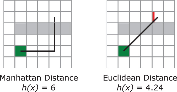
The Manhattan distance heuristic, illustrated in Figure 4.7 (left), is akin to traveling along city blocks in a sprawling metropolis. A building might be “five blocks away,” but there may be multiple routes five blocks in length. Manhattan distance assumes that diagonal movements are invalid. If diagonal movements are valid, Manhattan distance often overestimates the cost, making the heuristic inadmissible.
For a 2D grid, the following formula calculates Manhattan distance:
![]()
A second type of heuristic is Euclidean distance, illustrated in Figure 4.7 (right). You use the standard distance formula to calculate this heuristic, which estimates an “as the crow flies” route. Unlike Manhattan distance, Euclidean distance can easily work for worlds more complex than a square grid. In 2D, the Euclidean distance equation is as follows:
![]()
The Euclidean distance function is almost always admissible, even in cases where the Manhattan distance is inadmissible. This means that Euclidean distance is usually the recommended heuristic function. However, the Manhattan heuristic is more efficient to compute because it doesn’t involve a square root.
The only case where a Euclidean distance heuristic overestimates the true cost is if the game allows non-Euclidean movement such as teleporting between two nodes across the level.
Notice that in Figure 4.7 both heuristic h(x) functions end up underestimating the actual cost of traveling from the start node to the goal node. This happens because the heuristic function knows nothing about the adjacency lists, so it doesn’t know whether certain areas are impassible. This is fine because the heuristic is the lower bound of how close node x is to the goal node; the heuristic guarantees that node x is at least that distance away. This is more useful in a relative sense: The heuristic can help estimate whether node A or node B is closer to the goal node. And then you can use this estimate to help decide whether to explore node A or node B next.
The following section shows how to use the heuristic function to create a more complex pathfinding algorithm.
Greedy Best-First Search
BFS uses a queue to consider nodes in a FIFO manner. Greedy best-first search (GBFS) instead uses the h(x) heuristic function to decide which node to consider next. Although this seems like a reasonable pathfinding algorithm, GBFS cannot guarantee a minimal path. Figure 4.8 shows the resultant path from a sample GBFS search. Nodes in gray are impassible. Note that the path makes four additional moves from the start rather than going straight down.

note
Although GBFS does not guarantee optimality, it’s useful to understand because it requires only a couple modifications to become A*. The A* algorithm does guarantee the shortest path if the heuristic is admissible. So before moving on to A*, it’s important to understand the GBFS implementation.
Instead of using a single queue, GBFS uses two sets of nodes during the search. The open set contains the nodes that are under consideration. Once chosen for evaluation, a node moves into the closed set. When a node is in the closed set, GBFS need not investigate it further. There’s no guarantee that a node in the open or closed set will ultimately be on the path; these sets just help prune nodes from consideration.
Selecting data structures for the open set and the closed set presents an interesting dilemma. For the open set, the two operations you need are removing the node with the lowest cost and testing for membership. The closed set only needs a membership test. To speed up the membership test, you can simply use Booleans in scratch data to track if a specific node is a member of the open set or the closed set. And because the closed set just needed this membership test, you don’t use an actual collection for the closed set.
For the open set, one popular data structure is a priority queue. However, in the interest of simplicity, this chapter uses a vector for the open set. With a vector, you can just use a linear search to find the element in the open set with the lowest cost.
As with BFS, each node needs additional scratch data during the GBFS search. Because you now have multiple pieces of scratch data per node, it makes sense to define a struct to encapsulate it. To use a weighted graph, the parent is an incoming edge as opposed to a preceding node. In addition, each node tracks its heuristic value and its membership in the open and closed sets:
struct GBFSScratch
{
const WeightedEdge* mParentEdge = nullptr;
float mHeuristic = 0.0f;
bool mInOpenSet = false;
bool mInClosedSet = false;
};
Then, define a map where the key is a pointer to the node and the value is an instance of GBFSScratch:
using GBFSMap =
std::unordered_map<const WeightedGraphNode*, GBFSScratch>;
Now you have the necessary components for a greedy best-first search. The GBFS function takes in a WeightedGraph, the start node, the goal node, and a reference to a GBFSMap:
bool GBFS(const WeightedGraph& g, const WeightedGraphNode* start,
const WeightedGraphNode* goal, GBFSMap& outMap);
At the start of the GBFS function, you define a vector for the open set:
std::vector<const WeightedGraphNode*> closedSet;
Next, you need a variable to track the current node, which is the node under evaluation. This updates as the algorithm progresses. Initially, current is the start node, and you “add” it to the closed set by marking it as closed in the scratch map:
const WeightedGraphNode* current = start;
outMap[current].mInClosedSet = true;
Next, you enter the main loop of GBFS. This main loop does several things. First, it looks at all nodes adjacent to the current node. It only considers nodes that aren’t already in the closed set. These nodes have their parent edge set to the edge incoming from the current node. For nodes not already in the open set, the code computes the heuristic (from the node to the goal) and adds the node to the open set:
do
{
// Add adjacent nodes to open set
for (const WeightedEdge* edge : current->mEdges)
{
// Get scratch data for this node
GBFSScratch& data = outMap[edge->mTo];
// Add it only if it's not in the closed set
if (!data.mInClosedSet)
{
// Set the adjacent node's parent edge
data.mParentEdge = edge;
if (!data.mInOpenSet)
{
// Compute the heuristic for this node, and add to open set
data.mHeuristic = ComputeHeuristic(edge->mTo, goal);
data.mInOpenSet = true;
openSet.emplace_back(edge->mTo);
}
}
}
The ComputeHeuristic function can use any heuristic h(x) function, such as Manhattan or Euclidean distance. In practice, this may require additional information stored in each node (such as the position of the node in the world).
After processing the nodes adjacent to the current node, you need to look at the open set. If it’s empty, this means there are no nodes left to evaluate. This happens only if there is no path from start to goal:
if (openSet.empty())
{
break; // Break out of outer loop
}
Alternatively, if there are still nodes in the open set, the algorithm continues. You need to find the node in the open set with the lowest heuristic cost and move it to the closed set. This node becomes the new current node:
// Find lowest cost node in open set
auto iter = std::min_element(openSet.begin(), openSet.end(),
[&outMap](const WeightedGraphNode* a, const WeightedGraphNode* b)
{
return outMap[a].mHeuristic < outMap[b].mHeuristic;
});
// Set to current and move from open to closed
current = *iter;
openSet.erase(iter);
outMap[current].mInOpenSet = false;
outMap[current].mInClosedSet = true;
To code to find the lowest element, uses the std::min_element function from the <algorithm> header. For its third parameter, min_element takes in a special type of function (called a lambda expression) to specify how to decide whether one element is less than another. The min_element function returns an iterator to the minimum element.
Finally, the main loop continues if the current node is not the goal node:
} while (current != goal);
The loop terminates either when the above while condition fails or when you hit the earlier break statement (for when the open set is empty). You can then figure out if GBFS found a path based on whether the current node equals the goal node:
return (current == goal) ? true : false;
Figure 4.9 shows the first two iterations of GBFS applied to a sample data set. In Figure 4.9(a), the start node (A2) is in the closed set, and its adjacent nodes are in the open set. To make the figure easy to read, it uses the Manhattan distance heuristic. The arrows point from children back to their parent node. The next step is to select the node with the lowest heuristic cost, which is the node with h = 3. This node becomes the new current node and moves into the closed set. Figure 4.9(b) shows the next iteration, where C2 is now the node with the lowest cost in the open set.

Keep in mind that just because a node in the open set has the lowest heuristic cost doesn’t mean it’s on the optimal path. For example, in Figure 4.9(b), the node C2 is not on the optimal path. Unfortunately, the GBFS algorithm still selects C2 for its path. Clearly, you need to do some refinement to fix this issue.
Listing 4.3 shows the complete code for the greedy best-first search function.
Listing 4.3 Greedy Best-First Search
bool GBFS(const WeightedGraph& g, const WeightedGraphNode* start,
const WeightedGraphNode* goal, GBFSMap& outMap)
{
std::vector<const WeightedGraphNode*> openSet;
// Set current node to start, and mark in closed set
const WeightedGraphNode* current = start;
outMap[current].mInClosedSet = true;
do
{
// Add adjacent nodes to open set
for (const WeightedEdge* edge : current->mEdges)
{
// Get scratch data for this node
GBFSScratch& data = outMap[edge->mTo];
// Consider it only if it's not in the closed set
if (!data.mInClosedSet)
{
// Set the adjacent node's parent edge
data.mParentEdge = edge;
if (!data.mInOpenSet)
{
// Compute the heuristic for this node, and add to open set
data.mHeuristic = ComputeHeuristic(edge->mTo, goal);
data.mInOpenSet = true;
openSet.emplace_back(edge->mTo);
}
}
}
if (openSet.empty())
{ break; }
// Find lowest cost node in open set
auto iter = std::min_element(openSet.begin(), openSet.end(),
[&outMap](const WeightedGraphNode* a, const WeightedGraphNode* b)
{
return outMap[a].mHeuristic < outMap[b].mHeuristic;
});
// Set to current and move from open to closed
current = *iter;
openSet.erase(iter);
outMap[current].mInOpenSet = false;
outMap[current].mInClosedSet = true;
} while (current != goal);
// Did you find a path?
return (current == goal) ? true : false;
}
A* Search
The downside of GBFS is that it can’t guarantee an optimal path. Luckily, with some modifications to GBFS, you can transform it into the A* search (pronounced “A-star”). A* adds a path-cost component, which is the actual cost from the start node to a given node. The notation g(x) denotes the path-cost of a node x. When selecting a new current node, A* selects the node with the lowest f(x) value, which is just the sum of the g(x) path-cost and the h(x) heuristic for that node:
f (x)= g(x)+h(x)
There are a few conditions for A* to find an optimal path. Of course, there must be some path between the start and goal. Furthermore, the heuristic must be admissible (so it can’t overestimate the actual cost). Finally, all edge weights must be greater than or equal to zero.
To implement A*, you first define an AStarScratch struct, as you do for GBFS. The only difference is that the AStarScratch struct also has a float member mActualFromStart to store the g(x) value.
There are additional differences between the GBFS code and the A* code. When adding a node to the open set, A* must also compute the path-cost g(x). And when selecting the minimum node, A* selects the node with the lowest f(x) cost. Finally, A* is pickier about which nodes become parents, using a process called node adoption.
In the GBFS algorithm, adjacent nodes always have their parents set to the current node. But in A*, the g(x) path-cost value of a node is dependent on the g(x) value of its parent. This is because the path-cost value for node x is simply its parent’s path-cost value plus the cost of traversing the edge from the parent to node x. So before assigning a new parent to a node x, A* first makes sure the g(x) value will improve.
Figure 4.10(a) once again uses the Manhattan heuristic function. The current node (C3) checks its adjacent nodes. The node to its left has g = 2 and B2 as its parent. If that node instead had C3 as its parent, it would have g = 4, which is worse. So, A* will not change B2’s parent in this case.

Figure 4.10(b) shows the final path as computed by A*, which clearly is superior to the GBFS solution.
Apart from node adoption, the code for A* ends up being very similar to the GBFS code. Listing 4.4 shows the loop over the adjacent nodes, which contains most of the code changes. The only other change not shown in the text is the code that selects the lowest-cost node in the open set based on f(x) instead of just h(x). The game project for this chapter provides the code for the full A* implementation.
Listing 4.4 Loop over the Adjacent Nodes in an A* Search
for (const WeightedEdge* edge : current->mEdges)
{
const WeightedGraphNode* neighbor = edge->mTo;
// Get scratch data for this node
AStarScratch& data = outMap[neighbor];
// Only check nodes that aren't in the closed set
if (!data.mInClosedSet)
{
if (!data.mInOpenSet)
{
// Not in the open set, so parent must be current
data.mParentEdge = edge;
data.mHeuristic = ComputeHeuristic(neighbor, goal);
// Actual cost is the parent's plus cost of traversing edge
data.mActualFromStart = outMap[current].mActualFromStart +
edge->mWeight;
data.mInOpenSet = true;
openSet.emplace_back(neighbor);
}
else
{
// Compute what new actual cost is if current becomes parent
float newG = outMap[current].mActualFromStart + edge->mWeight;
if (newG < data.mActualFromStart)
{
// Current should adopt this node
data.mParentEdge = edge;
data.mActualFromStart = newG;
}
}
}
}
note
Optimizing A* to run as efficiently as possible is a complex topic. One consideration is what happens if there are a lot of ties in the open set. This is bound to happen in a square grid, especially if you use the Manhattan heuristic. If there are too many ties, when it’s time to select a node, you have a high probability of selecting one that doesn’t end up on the path. This ultimately means you need to explore more nodes in the graph, which makes A* run more slowly.
One way to help eliminate ties is to add a weight to the heuristic function, such as arbitrarily multiplying the heuristic by 0.75. This gives more weight to the path-cost g(x) function over the heuristic h(x) function, which means you’re more likely to explore nodes further from the start node.
From an efficiency standpoint, A* actually is a poor choice for grid-based pathfinding. Other pathfinding algorithms are far more efficient for grids. One of them is the JPS+ algorithm, outlined in Steve Rabin’s Game AI Pro 2 (see the “Additional Reading” section). However, A* works on any graph, whereas JPS+ works only on grids.
Dijkstra’s Algorithm
Let’s return to the maze example but now suppose that the maze has multiple pieces of cheese in it, and you want the mouse to move toward the closest cheese. A heuristic could approximate which cheese is closest, and A* could find a path to that cheese. But there’s a chance that the cheese you select with the heuristic isn’t actually the closest because the heuristic is only an estimate.
In Dijkstra’s algorithm, there is a source node but no goal node. Instead, Dijkstra’s computes the distance from the source node to every other reachable node in the graph. In the maze example, Dijkstra’s would find the distance of all reachable nodes from the mouse, yielding the actual cost of travel to every piece of cheese and allowing the mouse to move to the closest one.
It’s possible to convert the A* code from the previous section into Dijkstra’s. First, you remove the h(x) heuristic component. This is equivalent to a heuristic function of h(x) = 0, which is admissible because it’s guaranteed to be less than or equal to the actual cost. Next, you remove the goal node and make the loop terminate only when the open set is empty. This then computes the g(x) path-cost for every node reachable from the start.
The original formulation of the algorithm by Edsger Dijkstra is slightly different. But the approach proposed in this section is functionally equivalent to the original. (AI textbooks sometimes call this approach uniform cost search). Interestingly, the invention of Dijkstra’s algorithm predates GBFS and A*. However, games usually prefer heuristic-guided approaches such as A* because they generally search far fewer nodes than Dijkstra’s.
Following a Path
Once the pathfinding algorithm generates a path, the AI needs to follow it. You can abstract the path as a sequence of points. The AI then just moves from point to point in this path. You can implement this in a subclass of MoveComponent called NavComponent. Because MoveComponent can already move an actor forward, NavComponent only needs to rotate the actor to face the correct direction as the actor moves along the path.
First, the TurnTo function in NavComponent rotates the actor to face a point:
void NavComponent::TurnTo(const Vector2& pos)
{
// Vector from me to pos
Vector2 dir = pos - mOwner->GetPosition();
// New angle is just atan2 of this dir vector
// (Negate y because +y is down on screen)
float angle = Math::Atan2(-dir.y, dir.x);
mOwner->SetRotation(angle);
}
Next, NavComponent has a mNextPoint variable that tracks the next point in the path. The Update function tests whether the actor reaches mNextPoint:
void NavComponent::Update(float deltaTime)
{
// If you've reached the next point, advance along path
Vector2 diff = mOwner->GetPosition() - mNextPoint;
if (diff.Length() <= 2.0f)
{
mNextPoint = GetNextPoint();
TurnTo(mNextPoint);
}
// This moves the actor forward
MoveComponent::Update(deltaTime);
}
This assumes that the GetNextPoint function returns the next point on the path. Assuming that the actor starts at the first point on the path, initializing mNextPoint to the second point as well as setting a linear speed gets the actor moving along the path.
There’s one issue with updating the movement along the path in this way: It assumes that the actor is not moving so fast that it jumps too far past a node in one step. If this happens, the distance between the two will never be close enough, and the actor will get lost.
Other Graph Representations
For a game with real-time action, non-player characters (NPCs) usually don’t move from square to square on a grid. This makes it more complex to represent the world with a graph. This section discusses two alternative approaches: using path nodes and using navigation meshes.
Path nodes (also called waypoint graphs) became popular with the advent of first-person shooter (FPS) games in the early 1990s. With this approach, a designer places path nodes at locations in the game world that the AI can path to. These path nodes directly translate into nodes in the graph.
Typically, you generate the edges between path nodes automatically. The algorithm works as follows: For each path node, test whether there are obstructions between it and nearby nodes. Any paths without obstructions yield edges. A line segment cast or similar collision test can determine if there are obstructions. Chapter 10, “Collision Detection,” covers how to implement line segment casts.
The primary drawback of using path nodes is that the AI can only move to locations on the nodes or edges. This is because even if path nodes form a triangle, there is no guarantee that the interior of the triangle is a valid location. There may be an obstruction in the way, so the pathfinding algorithm must assume that any location not on a node or an edge is invalid.
In practice, this means that either there’s a lot of space in the world that’s off-limits to AI or you need many path nodes. The first is undesirable because it results in less believable behavior from the AI, and the second is simply inefficient. The more nodes and more edges there are, the longer it takes a pathfinding algorithm to arrive at a solution. This presents a trade-off between performance and accuracy.
Other games use a navigation mesh (or nav mesh). In this approach, each node in the graph corresponds to a convex polygon. Adjacent nodes are any adjacent convex polygons. This means that a handful of convex polygons can represent entire regions in the game world. With a navigation mesh, the AI can safely travel to any location inside a convex polygon node. This means the AI has improved maneuverability. Figure 4.11 compares the path node and navigation mesh representations of a location in a game.

Navigation meshes also better support characters of different sizes. Suppose a game has both cows and chickens walking around a farm. Given that chickens are smaller than cows, there are some areas that are accessible to chickens but not to cows. Therefore, a path node network designed for chickens won’t work correctly for cows. This means that if the game uses path nodes, it needs two separate graphs: one for each type of creature. In contrast, each node in a navigation mesh is a convex polygon, so it’s possible to calculate whether a character fits in a specific area. Therefore, the game can use a single navigation mesh for both chickens and cows.
Most games that use navigation meshes automatically generate them. This is useful because designers can change a level without worrying much about the effect on AI pathing. However, navigation mesh generation algorithms are complex. Luckily, there are open source libraries that implement nav mesh generation. The most popular, Recast, generates a navigation mesh given the triangle geometry of a 3D level. See the “Additional Reading” section at the end of this chapter for more information on Recast.
Game Trees
Games such as tic-tac-toe or chess are very different from most real-time games. First, the game has two players, and each player alternates taking a turn. Second, the game is adversarial, meaning that the two players are playing against each other. The AI needs for these types of games are very different from those of real-time games. These types of games require some representation of the overall game state, and this state informs the AI’s decisions. One approach is to use a tree called a game tree. In a game tree, the root node represents the current state of the game. Each edge represents a move in the game and leads to a new game state.
Figure 4.12 shows a game tree for an in-progress game of tic-tac-toe. Starting at the root node, the current player (called the max player) can select from three different moves. After the max player makes a move, the game state transitions to a node in the first level of the tree. The opponent (called the min player) then selects a move leading to the second level of the tree. This process repeats until reaching a leaf node, which represents an end state of the game.

In tic-tac-toe, there are only three outcomes: win, lose, or draw. The numeric values assigned to the leaf nodes in Figure 4.12 reflect these outcomes. These values are scores from the perspective of the max player: 1 means the max player wins, -1 means the min player wins, and 0 means a tie.
Different games have different state representations. For tic-tac-toe, the state is simply a 2D array of the board:
struct GameState
{
enum SquareState { Empty, X, O };
SquareState mBoard[3][3];
};
A game tree node stores both a list of children as well as the game state at that node:
struct GTNode
{
// Children nodes
std::vector<GTNode*> mChildren;
// State of game at this node
GameState mState;
};
To generate a complete game tree, you set the root node to the current game state and create children for each possible first move. Then you repeat this process for each node in the first level and continue until all moves are exhausted.
The size of a game tree grows exponentially based on the number of potential moves. For tic-tac-toe, the upper bound of the game tree is 9!, or 362,880 nodes. This means it’s possible to generate and evaluate a complete game tree for tic-tac-toe. But for chess, a complete game tree would have 10120 nodes, which makes it impossible to fully evaluate (both in terms of time and space complexity). For now, let’s assume we have a complete game tree. Later, we’ll discuss how to manage an incomplete tree.
Minimax
The minimax algorithm evaluates a two-player game tree to determine the best move for the current player. Minimax assumes that each player will make the choice most beneficial to herself. Because scores are from the perspective of the max player, this means the max player tries to maximize her score, while the min player strives to minimize the score of the max player.
For example, in Figure 4.12 the max player (X in this case) has three possible moves. If max selects either top-mid or bottom-mid, the min player (O) can win with bottom-right. The min player would take this winning play when available. Thus, the max player selects bottom-right to maximize her potential final score.
If the max player selects bottom-right, the min player can select either top-mid or bottom-mid. The choice here is between a score of 1 or 0. Because the min player aims to minimize the max player’s score, min selects bottom-mid. This means the game ends in a tie, which is the expected result of a game of tic-tac-toe where both players play optimally.
The implementation of minimax in Listing 4.5 uses a separate function for the min and max players’ behavior. Both functions first test if the node is a leaf node, in which case the GetScore function computes the score. Next, both functions determine the best possible subtree using recursion. For the max player, the best subtree yields the highest value. Likewise, the min player finds the subtree with the lowest value.
Listing 4.5 MaxPlayer and MinPlayer Functions
float MaxPlayer(const GTNode* node)
{
// If this is a leaf, return score
if (node->mChildren.empty())
{
return GetScore(node->mState);
}
// Find the subtree with the maximum value
float maxValue = -std::numeric_limits<float>::infinity();
for (const GTNode* child : node->mChildren)
{
maxValue = std::max(maxValue, MinPlayer(child));
}
return maxValue;
}
float MinPlayer(const GTNode* node)
{
// If this is a leaf, return score
if (node->mChildren.empty())
{
return GetScore(node->mState);
}
// Find the subtree with the minimum value
float minValue = std::numeric_limits<float>::infinity();
for (const GTNode* child : node->mChildren)
{
minValue = std::min(minValue, MaxPlayer(child));
}
return minValue;
}
Calling MaxPlayer on the root node returns the best possible score for the max player. However, this doesn’t specify which next move is optimal, which the AI player also wants to know. The code for determining the best move is in a separate MinimaxDecide function, given in Listing 4.6. MinimaxDecide resembles the MaxPlayer function, except it tracks which child yields the best value.
Listing 4.6 MinimaxDecide Implementation
const GTNode* MinimaxDecide(const GTNode* root)
{
// Find the subtree with the maximum value, and save the choice
const GTNode* choice = nullptr;
float maxValue = -std::numeric_limits<float>::infinity();
for (const GTNode* child : root->mChildren)
{
float v = MinPlayer(child);
if (v > maxValue)
{
maxValue = v;
choice = child;
}
}
return choice;
}
Handling Incomplete Game Trees
As mentioned earlier in this chapter, it’s not always viable to generate a complete game tree. Luckily, it’s possible to modify the minimax code to account for incomplete game trees. First, the functions must operate on a game state as opposed to a node. Next, rather than iterate over child nodes, the code iterates over the next possible moves from a given state. These modifications mean the minimax algorithm generates the tree during execution rather than beforehand.
If the tree is too large, such as in chess, it’s still not possible to generate the entire tree. Much as how an expert chess player can see only eight moves ahead, the AI needs to limit the depth of its game tree. This means the code treats some nodes as leaves even though they are not terminal states of the game.
To make informed decisions, minimax needs to know how good these nonterminal states are. But unlike with terminal states, it’s impossible to know the exact score. Thus, the scoring function needs a heuristic component that approximates the quality of nonterminal states. This also means that scores are now ranges of values, unlike the {-1, 0, 1} ternary choice for tic-tac-toe.
Importantly, adding the heuristic component means minimax cannot guarantee to make the best decision. The heuristic tries to approximate the quality of a game state, but it’s unknown how accurate this approximation is. With an incomplete game tree, it’s possible that the move selected by minimax is suboptimal and eventually leads to a loss.
Listing 4.7 provides the MaxPlayerLimit function. (You would need to modify the other functions similarly.) This code assumes that GameState has three member functions: IsTerminal, GetScore, and GetPossibleMoves. IsTerminal returns true if the state is an end state. GetScore returns either the heuristic for nonterminal states or the score for terminal states. GetPossibleMoves returns a vector of the game states that are one move after the current state.
Listing 4.7 MaxPlayerLimit Implementation
float MaxPlayerLimit(const GameState* state, int depth)
{
// If this is terminal or we've gone max depth
if (depth == 0 || state->IsTerminal())
{
return state->GetScore();
}
// Find the subtree with the max value
float maxValue = -std::numeric_limits<float>::infinity();
for (const GameState* child : state->GetPossibleMoves())
{
maxValue = std::max(maxValue, MinPlayer(child, depth - 1));
}
return maxValue;
}
The heuristic function varies depending on the game. For example, a simple chess heuristic might count the number of pieces each player has, weighting the pieces by power. However, a drawback of such a simple heuristic is that sometimes sacrificing a piece in the short term is better for the long term. Other heuristics might look at control of the board’s center, the safety of the king, or the mobility of the queen. Ultimately, several different factors affect the heuristic.
More complex heuristics require more calculations. Most games institute some sort of time limit for AI moves. For example, a chess game AI might have only 10 seconds to decide its next move. This makes it necessary to strike a balance between the depth explored and heuristic complexity.
Alpha-Beta Pruning
Alpha-beta pruning is an optimization of the minimax algorithm that, on average, reduces the number of nodes evaluated. In practice, this means it’s possible to increase the maximum depth explored without increasing the computation time.
Figure 4.13 shows a game tree simplified by alpha-beta pruning. Assuming a left-to-right order of evaluation for siblings, the max player first inspects subtree B. The min player then sees the leaf with value 5, which means the min player has a choice between 5 and other values. If these other values are greater than 5, the min player obviously selects 5. This means that the upper bound of subtree B is 5, but the lower bound is negative infinity. The min player continues and sees the leaf with value 0 and selects this leaf because the min player wants the minimum possible score.

Control returns to the max player function, which now knows that subtree B has a value of 0. Next, the max player inspects subtree C. The min player first sees the leaf with value -3. As before, this means the upper bound of subtree C is -3. However, you already know that subtree B has a value of 0, which is better than -3. This means that there’s no way subtree C can be better for the max player than subtree B. Alpha-beta pruning recognizes this and, as a result, does not inspect any other children of C.
Alpha-beta pruning adds two additional variables, called alpha and beta. Alpha is the best score guaranteed for the max player at the current level or higher. Conversely, beta is the best score guaranteed for the min player at the current level or higher. In other words, alpha and beta are the lower and upper bounds of the score.
Initially, alpha is negative infinity and beta is positive infinity—the worst possible values for both players. AlphaBetaDecide, in Listing 4.8, initializes alpha and beta to these values and then recurses by calling AlphaBetaMin.
Listing 4.8 AlphaBetaDecide Implementation
const GameState* AlphaBetaDecide(const GameState* root, int maxDepth)
{
const GameState* choice = nullptr;
// Alpha starts at negative infinity, beta at positive infinity
float maxValue = -std::numeric_limits<float>::infinity();
float beta = std::numeric_limits<float>::infinity();
for (const GameState* child : root->GetPossibleMoves())
{
float v = AlphaBetaMin(child, maxDepth - 1, maxValue, beta);
if (v > maxValue)
{
maxValue = v;
choice = child;
}
}
return choice;
}
The implementation of AlphaBetaMax, shown in Listing 4.9, builds on MaxPlayerLimit. If on any iteration the max value is greater than or equal to beta, it means the score can be no better than the previous upper bound. This makes it unnecessary to test the remaining siblings, and so the function returns. Otherwise, the code increases the alpha lower bound if the max value is greater than alpha.
Listing 4.9 AlphaBetaMax Implementation
float AlphaBetaMax(const GameState* node, int depth, float alpha,
float beta)
{
if (depth == 0 || node->IsTerminal())
{
return node->GetScore();
}
float maxValue = -std::numeric_limits<float>::infinity();
for (const GameState* child : node->GetPossibleMoves())
{
maxValue = std::max(maxValue,
AlphaBetaMin(child, depth - 1, alpha, beta));
if (maxValue >= beta)
{
return maxValue; // Beta prune
}
alpha = std::max(maxValue, alpha); // Increase lower bound
}
return maxValue;
}
Similarly, AlphaBetaMin, shown in Listing 4.10, checks whether the min value is less than or equal to alpha. In this case, the score can be no better than the lower bound, so the function returns. Then the code decreases the beta upper bound as necessary.
Listing 4.10 AlphaBetaMin Implementation
float AlphaBetaMin(const GameState* node, int depth, float alpha,
float beta)
{
if (depth == 0 || node->IsTerminal())
{
return node->GetScore();
}
float minValue = std::numeric_limits<float>::infinity();
for (const GameState* child : node->GetPossibleMoves())
{
minValue = std::min(minValue,
AlphaBetaMax(child, depth - 1, alpha, beta));
if (minValue <= alpha)
{
return minValue; // Alpha prune
}
beta = std::min(minValue, beta); // Decrease upper bound
}
return minValue;
}
Note that the order of evaluation for children affects the number of nodes pruned. This means that even with a consistent depth limit, different starting states yield different execution times. This can be problematic if the AI has a fixed time limit; an incomplete search means the AI has no idea which move to take. One solution is iterative deepening, which runs the algorithm multiple times at increasing depth limits. For example, first run alpha-beta pruning with a depth limit of three, which yields some baseline move. Then run with a depth limit of four, then five, and so on, until time runs out. At this point, the code returns the move from the previous iteration. This guarantees that some move is always available, even when time runs out.
Game Project
This chapter’s game project, shown in Figure 4.14, is a tower defense game. In this style of game, the enemies try to move from the start tile on the left to an end tile on the right. Initially, the enemies move in a straight line from left to right. However, the player can build towers on squares in the grid, even where the path is, which causes the path to redirect around these towers as needed. The code is available in the book’s GitHub repository, in the Chapter04 directory. Open Chapter04-windows.sln on Windows and Chapter04-mac.xcodeproj on Mac.

Figure 4.14 Chapter 4 game project
Use the mouse to click on and select tiles. After selecting a tile, use the B key to build a tower. The enemy airplanes path around the towers using the A* pathfinding algorithm. Each new tower built changes the path as necessary. To ensure that the player can’t fully block in the enemies, when the player requests to build a tower, the code first ensures that a path would still exist for the enemies. If a tower would completely block the path, the game doesn’t let the player build it.
As a simplification, the Tile class in the game project contains all the graph information, as well as the scratch data used by the A* search. The code that creates all the tiles and initializes the graph is in the constructor of the Grid class. The Grid class also contains the FindPath function that runs the actual A* search.
For completeness, the source code for this chapter also includes the versions of the search and minimax algorithms covered in the text in a separate Search.cpp file. It also includes the implementation of AIState and AIComponent, even though no actors in the game project use these features.
Summary
Artificial intelligence is a deep topic with many different sub-areas. Using state machines is an effective way to give behaviors to AI-controlled characters in a game. While a switch is the simplest implementation of a state machine, the state design pattern adds flexibility by making each state a separate class.
Pathfinding algorithms find the shortest path between two points in the game world. First, you formulate a graph representation for the game world. For a square grid, this is simple, but other games use path nodes or navigation meshes. For unweighted graphs, breadth-first search (BFS) guarantees to find the shortest path if one exists. But for weighted graphs, you need other algorithms, such as A* or Dijkstra’s, to find the shortest path.
For two-player adversarial turn-based games such as checkers or chess, a game tree represents the sequence of possible moves from the current game state. The minimax algorithm assumes that the current player aims to maximize his or her score, and the opponent aims to minimize the current player’s score. Alpha-beta pruning optimizes minimax, though for most games the tree must have a depth limit.
Additional Reading
Many resources cover AI techniques. Stuart Russell and Peter Norvig’s book is a popular AI text that covers many techniques, though only some are applicable to games. Mat Buckland’s book, although dated, covers many useful game AI topics. Steve Rabin’s Game AI Pro series has many interesting articles written by different game AI developers.
For navigation meshes, Stephen Pratt’s in-depth web article covers the steps to generate a navigation mesh from level geometry. The Recast project provides an open source implementation of both navigation mesh generation and pathfinding algorithms.
Buckland, Mat. Programming Game AI by Example. Plano: Wordware Publishing, 2005.
Mononen, Mikko. “Recast Navigation Mesh Toolkit.” Accessed July 7, 2017. https://github.com/recastnavigation.
Pratt, Stephen. “Study: Navigation Mesh Generation.” Accessed July 7, 2017. http://critterai.org/projects/nmgen_study/index.html.
Rabin, Steve, Ed. Game AI Pro 3: Collected Wisdom of Game AI Professionals. Boca Raton: CRC Press, 2017.
Russell, Stuart, and Peter Norvig. Artificial Intelligence: A Modern Approach, 3rd edition. Upper Saddle River: Pearson, 2009.
Exercises
The two exercises for this chapter implement techniques not used in this chapter’s game project. The first looks at state machines, and the second uses alpha-beta pruning for a four-in-a-row game.
Exercise 4.1
Given this chapter’s game project code, update either the Enemy or Tower class (or both!) to use an AI state machine. First, consider which behaviors the AI should have and design the state machine graph. Next, use the provided AIComponent and AIState base classes to implement these behaviors.
Exercise 4.2
In a four-in-a-row game, players have a vertical grid of six rows and seven columns. The two players take turns putting a piece at the top of a column, and then the piece slides down to the lowest free position in the column. The game continues until one player gets four in a row horizontally, vertically, or diagonally.
The starting code in Exercises/4.2 allows the human player to click to make a move. In the starting code, the AI randomly selects a move from the set of valid moves. Modify the AI code to instead use alpha-beta pruning with a depth cutoff.