
Chapter 12
Skeletal Animation
Animating characters for a 3D game is very different from animating characters for a 2D game. This chapter looks at skeletal animation, the most common animation used in 3D games. This chapter first goes over the mathematical foundations of the approach and then dives into the implementation details.
Foundations of Skeletal Animation
As described in Chapter 2, “Game Objects and 2D Graphics,” for 2D animation, games use a sequence of image files to yield the illusion of an animated character. A naïve solution for animating 3D characters is similar: Construct a sequence of 3D models and render those different models in rapid succession. Although this solution conceptually works, it’s not a very practical approach.
Consider a character model composed of 15,000 triangles, which is a conservative number for a modern game. Assuming only 10 bytes per vertex, the total memory usage of this one model might be around 50 to 100 KB. A two-second animation running at 30 frames per second would need a total of 60 different models. This means the total memory usage for this single animation would be 3 to 6 MB. Now imagine that the game uses several different animations and several different character models. The memory usage for the game’s models and animations will quickly become too high.
In addition, if a game has 20 different humanoid characters, chances are their movements during an animation such as running are largely the same. If you use the naïve solution just described, each of these 20 characters needs a different model set for its animations. This also means that artists need to manually author these different model sets and animations for each character.
Because of these issues, most 3D games instead take inspiration from anatomy: vertebrates, like humans, have bones. Attached to these bones are muscles, skin, and other tissue. Bones are rigid, while the other tissues are not. Thus, given the position of a bone, it’s possible to derive the position of the tissue attached to the bone.
Similarly, in skeletal animation, the character has an underlying rigid skeleton. This skeleton is what the animator animates. Then, each vertex in the model has an association with one or more bones in the skeleton. When the animation moves the bones, the vertices deform around the associated bones (much the way your skin stretches when you move around). This means that there only needs to be a single 3D model for a character, regardless of the number of animations for the model.
note
Because skeletal animation has bones and vertices that deform along the bones, some call this technique skinned animation. The “skin” in this case is the model’s vertices.
Similarly, the terms bone and joint, though different in the context of anatomy, are interchangeable terms in the context of skeletal animation.
An advantage of skeletal animation is that the same skeleton can work for several different characters. For example, it’s common in a game for all humanoid characters to share the same skeleton. This way, the animator creates one set of animations for the skeleton, and all characters can then use those animations.
Furthermore, many popular 3D model authoring programs such as Autodesk Maya and Blender support skeletal animations. Thus, artists can use these tools to author the skeletons and animations for characters. Then, as with 3D models, you can write exporter plugins to export into the preferred format for the game code. As with 3D models this book uses a JSON-based file format for the skeleton and animations. (As a reminder, the book’s code on GitHub includes an exporter for Epic Games’s Unreal Engine, in the Exporter directory.)
The remainder of this section looks at the high-level concepts and mathematics that drive skeletal animation. The subsequent section then dives into the details of implementing skeletal animation in game code.
Skeletons and Poses
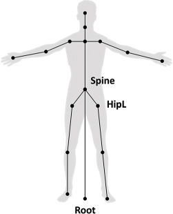
The usual representation of a skeleton is as a hierarchy (or tree) of bones. The root bone is the base of the hierarchy and has no parent bone. Every other bone in the skeleton has a single parent bone. Figure 12.1 illustrates a simple skeletal hierarchy for a humanoid character. The spine bone is a child of the root bone, and then in turn the left and right hip bones are children of the spine bone.
This bone hierarchy attempts to emulate anatomy. For example, if a human rotates her shoulder, the rest of the arm follows that rotation. With a game skeleton, you might represent this by saying the shoulder bone is the parent of the elbow bone, the elbow bone is the parent of the wrist bone, and the wrist bone is the parent of the finger bones.
Given a skeleton, a pose represents a configuration of the skeleton. For example, if a character waves hello in an animation, there is one pose during the animation where the character’s hand bone is raised up to wave. An animation is then just a sequence of poses the skeleton transitions between over time.
The bind pose is the default pose of the skeleton, prior to applying any animation. Another term for bind pose is t-pose because, typically, the character’s body forms a T shape in bind pose, as in Figure 12.1. You author a character’s model so that it looks like this bind pose configuration.
The reason the bind pose usually looks like a T because it makes it easier to associate bones to vertices, as discussed later in this chapter.
In addition to specifying the parent/child relationships of the bones in the skeleton, you also must specify each bone’s position and orientation. Recall that in a 3D model, each vertex has a position relative to the object space origin of the model. In the case of a humanoid character, a common placement of the object space origin is between the feet of the character in bind pose. It’s not accidental that this also corresponds to the typical placement of the root bone of the skeleton.
For each bone in the skeleton, you can describe its position and orientation in two ways. A global pose is relative to the object space origin. Conversely, a local pose is relative to a parent bone. Because the root bone has no parent, its local pose and global pose are identical. In other words, the position and orientation of the root bone is always relative to the object space origin.
Suppose that you store local pose data for all the bones. One way to represent position and orientation is with a transform matrix. Given a point in the bone’s coordinate space, this local pose matrix would transform the point into the parent’s coordinate space.
If each bone has a local pose matrix, then given the parent/child relationships of the hierarchy, you can always calculate the global pose matrix for any bone. For example, the parent of the spine is the root bone, so its local pose matrix is its position and orientation relative to the root bone. As established, the root bone’s local pose matrix corresponds to its global pose matrix. So multiplying the local pose matrix of the spine by the root bone’s global pose matrix yields the global pose matrix for the spine:
![]()
With the spine’s global pose matrix, given a point in the spine’s coordinate space, you could transform it into object space.
Similarly, to compute the global pose matrix of the left hip, whose parent is the spine, the calculation is as follows:
![]()
Because you can always convert from local poses to global poses, it may seem reasonable to store only local poses. However, by storing some information in global form, you can reduce the number of calculations required every frame.
Although storing bone poses with matrices can work, much as with actors, you may want to separate the bone position and orientation into a vector for the translation and a quaternion for the rotation. The main reason to do this is that quaternions allow for more accurate interpolation of the rotation of a bone during an animation. You can omit a scale for the bones because scaling bones typically only sees use for cartoon-style characters who can stretch in odd ways.
You can combine the position and orientation into the following BoneTransform struct:
struct BoneTransform
{
Quaternion mRotation;
Vector3 mTranslation;
// Convert to matrix
Matrix4 ToMatrix() const;
};
The ToMatrix function converts the transform into a matrix. This just creates rotation and translation matrices from the member data and multiplies these matrices together. This function is necessary because even though many intermediate calculations directly use the quaternion and vector variables, ultimately the graphics code and shaders need matrices.
To define the overall skeleton, for each bone you need to know the name of the bone, the parent of the bone, and its bone transform. For the bone transform, you specifically store the local pose (the transform from the parent) when the overall skeleton is in the bind pose.
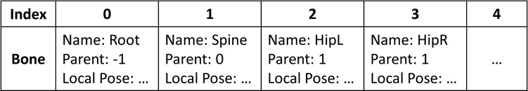
One way to store these bones is in an array. Index 0 of the array corresponds to the root bone, and then each subsequent bone references its parent by an index number. For the example in Figure 12.2, the spine bone, stored in index 1, has a parent index of 0 because the root bone is its parent. Similarly, the hip bone, stored in index 2, has a parent of index 1.
This leads to the following Bone struct that contains the local bind pose transform, a bone name, and a parent index:
struct Bone
{
BoneTransform mLocalBindPose;
std::string mName;
int mParent;
};
Then, you define a std::vector of bones that you can fill in based on the skeleton. The root bone sets its parent index to -1, but every other bone has a parent indexing into the array. To simplify later calculations, parents should be at earlier indices in the array than their children bones. For example, because the left hip is a child of spine, it should never be the case that left hip has a lower index than spine.
The JSON-based file format used to store the skeleton data directly mirrors this representation. Listing 12.1 gives a snippet of a skeleton file, showing the first two bones: root and pelvis.
Listing 12.1 The Beginning of a Skeleton Data File
{
"version":1,
"bonecount":68,
"bones":[
{
"name":"root",
"parent":-1,
"bindpose":{
"rot":[0.000000,0.000000,0.000000,1.000000],
"trans":[0.000000,0.000000,0.000000]
}
},
{
"name":"pelvis",
"parent":0,
"bindpose":{
"rot":[0.001285,0.707106,-0.001285,-0.707106],
"trans":[0.000000,-1.056153,96.750603]
}
},
// ...
]
}
The Inverse Bind Pose Matrix
With the local bind pose information stored in the skeleton, you can easily compute a global bind pose matrix for every bone by using matrix multiplication, as shown earlier. Given a point in a bone’s coordinate space, multiplying by this global bind pose matrix yields that point transformed into object space. This assumes that the skeleton is in the bind pose.
The inverse bind pose matrix for a bone is simply the inverse of the global bind pose matrix. Given a point in object space, multiplying it by the inverse bind pose matrix yields that point transformed into the bone’s coordinate space. This is actually very useful because the model’s vertices are in object space, and the models’ vertices are in the bind pose configuration. Thus, the inverse bind pose matrix allows you to transform a vertex from the model into a specific bone’s coordinate space (in bind pose).
For example, you can compute the spine bone’s global bind pose matrix with this:
![]()
Its inverse bind pose matrix is then simply as follows:
![]()
The simplest way to compute the inverse bind pose matrix is in two passes. First, you compute each bone’s global bind pose matrix using the multiplication procedure from the previous section. Second, you invert each of these matrices to get the inverse bind pose.
Because the inverse bind pose matrix for each bone never changes, you can compute these matrices when loading the skeleton.
Animation Data
Much the way you describe the bind pose of a skeleton in terms of local poses for each of the bones, you can describe any arbitrary pose. More formally, the current pose of a skeleton is just the set of local poses for each bone. An animation is then simply a sequence of poses played over time. As with the bind pose, you can convert these local poses into global pose matrices for each bone, as needed.
You can store this animation data as a 2D dynamic array of bone transforms. In this case, the row corresponds to the bone, and the column corresponds to the frame of the animation.
One issue with storing animation on a per-frame basis is that the frame rate of the animation may not correspond to the frame rate of the game. For example, the game may update at 60 FPS, but the animation may update at 30 FPS. If the animation code tracks the duration of the animation, then every frame, you can update this by delta time. However, it will sometimes be the case that the game needs to show the animation between two different frames. To support this, you can add a static Interpolate function to BoneTransform:
BoneTransform BoneTransform::Interpolate(const BoneTransform& a,
const BoneTransform& b, float f)
{
BoneTransform retVal;
retVal.mRotation = Quaternion::Slerp(a.mRotation, b.mRotation, f);
retVal.mTranslation = Vector3::Lerp(a.mTranslation,
b.mTranslation, f);
return retVal;
}
Then, if the game must show a state between two different frames, you can interpolate the transforms of each bone to get the current local pose.
Skinning
Skinning involves associating vertices in the 3D model with one or more bones in the corresponding skeleton. (This is different from the term skinning in a non-animation context.) Then, when drawing a vertex, the position and orientation of any associated bones influence the position of the vertex. Because the skinning of a model does not change during the game, the skinning information is an attribute of each vertex.
In a typical implementation of skinning, each vertex can have associations with up to four different bones. Each of these associations has a weight, which designates how much each of the four bones influences the vertex. These weights must sum to one. For example, the spine and left hip bone might influence a vertex on the lower-left part of the torso of the character. If the vertex is closer to the spine, it might have a weight of 0.7 for the spline bone and 0.3 for the hip bone. If a vertex has only one bone that influences it, as is common, then that one bone simply has a weight of 1.0.
For the moment, don’t worry about how to add these additional vertex attributes for both the bones and skinning weights. Instead, consider the example of a vertex that has only one bone influencing it. Remember that the vertices stored in the vertex buffer are in object space, while the model is in bind pose. But if you want to draw the model in an arbitrary pose, P, you must then transform each vertex from object space bind pose into object space in the current pose, P.
To make this example concrete, suppose that the sole bone influence of vertex v is the spine bone. You already know the inverse bind pose matrix for the spine from earlier calculations. In addition, from the animation data, you can calculate the spine’s global pose matrix for the current pose, P. To transform v into object space of the current pose, you first transform it into the local space of the spine in bind pose. Then you transform it into object space of the current pose. Mathematically, it looks like this:
![]()
Now, suppose that v instead has two bone influences: The spine has a weight of 0.75, and the left hip has a weight of 0.25. To calculate v in the current pose in this case, you need to calculate each bone’s current pose vertex position separately and then interpolate between them, using these weights:
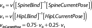
You could similarly extend the calculation for a vertex with four different bone influences.
Some bones, such as the spine, influence hundreds of vertices on the character model. Recalculating the multiplication between the spine’s inverse bind pose matrix and the current pose matrix for each of these vertices is redundant. On a single frame, the result of this multiplication will never change. The solution is to create an array of matrices called the matrix palette. Each index in this array contains the result of the multiplication between the inverse bind pose matrix and the current pose matrix for the bone with the corresponding index.
For example, if the spine is at index 1 in the bone array, then index 1 of the matrix palette contains the following:
![]()
Any vertex that’s influenced by the spine can then use the precomputed matrix from the palette. For the case of the vertex solely influenced by the spine, its transformed position is as follows:
![]()
Using this matrix palette saves thousands of extra matrix multiplications per frame.
Implementing Skeletal Animation
With the mathematical foundations established, you can now add skeletal animation support to the game. First, you add support for the additional vertex attributes that a skinned model needs (bone influences and weights), and then you draw the model in bind pose. Next, you add support for loading the skeleton and compute the inverse bind pose for each bone. Then, you can calculate the current pose matrices of an animation and save the matrix palette. This allows you to draw the model in the first frame of an animation. Finally, you add support for updating the animation based on delta time.
Drawing with Skinning Vertex Attributes
Although drawing a model with different vertex attributes seems straightforward, several pieces of code written in Chapter 6, “3D Graphics,” assume a single vertex layout. Recall that to this point, all 3D models have used a vertex layout with a position, a normal, and texture coordinates. To add support for the new skinning vertex attributes, you need to make a nontrivial number of changes.
First, you create a new vertex shader called Skinned.vert. Recall that you write shaders in GLSL, not C++. You don’t need a new fragment shader in this case because you still want to light the pixels with the Phong fragment shader from Chapter 6. Initially, Skinned.vert is just a copy of Phong.vert. Recall that the vertex shader must specify the expected vertex layout of each incoming vertex. Thus, you must change the declaration of the vertex layout in Skinned.vert to the following:
layout(location = 0) in vec3 inPosition;
layout(location = 1) in vec3 inNormal;
layout(location = 2) in uvec4 inSkinBones;
layout(location = 3) in vec4 inSkinWeights;
layout(location = 4) in vec2 inTexCoord;
This set of declarations says that you expect the vertex layout to have three floats for position, three floats for the normal, four unsigned integers for the bones that influence the vertex, four floats for the weights of these bone influences, and two floats for the texture coordinates.
The previous vertex layout—with position, normal, and texture coordinates—uses single-precision floats (4 bytes each) for all the values. Thus, the old vertex layout has a size of 32 bytes. If you were to use single-precision floats for the skinning weights and full 32-bit integers for the skinned bones, this would add an additional 32 bytes, doubling the size of each vertex in memory.
Instead, you can limit the number of bones in a model to 256. This means you only need a range of 0 to 255 for each bone influence—or a single byte each. This reduces the size of inSkinBones from 16 bytes to 4 bytes. In addition, you can specify that the skinning weights will also be in a range of 0 to 255. OpenGL can then automatically convert this 0–255 range to a normalized floating-point range of 0.0–1.0. This reduces the size of inSkinWeights to 4 bytes, as well. This means that, in total, the size of each vertex will be the original 32 bytes, plus an additional 8 bytes for the skinned bones and weights. Figure 12.3 illustrates this layout.

To reduce the memory usage of inSkinBones and inSkinWeights, you don’t need to make any further changes to the shader code. Instead, you need to specify the expected sizes of these attributes when defining the vertex array attributes in your C++ code. Recall from Chapter 5, “OpenGL,” that the definition of the vertex array attributes occurs in the VertexArray constructor. To support different types of vertex layouts, you add a new enum to the declaration of the VertexArray class in VertexArray.h:
enum Layout
{
PosNormTex,
PosNormSkinTex
};
Then, you modify the VertexArray constructor so that it takes in a Layout as a parameter. Then, in the code for the constructor you check the layout to determine how to define the vertex array attributes. For the case of PosNormTex, you use the previously written vertex attribute code. Otherwise, if the layout is PosNormSkinTex, you define the layout as in Listing 12.2.
Listing 12.2 Declaring Vertex Attributes in the VertexArray Constructor
if (layout == PosNormTex)
{ /* From Chapter 6... */ }
else if (layout == PosNormSkinTex)
{
// Position is 3 floats
glEnableVertexAttribArray(0);
glVertexAttribPointer(0, 3, GL_FLOAT, GL_FALSE, vertexSize, 0);
// Normal is 3 floats
glEnableVertexAttribArray(1);
glVertexAttribPointer(1, 3, GL_FLOAT, GL_FALSE, vertexSize,
reinterpret_cast<void*>(sizeof(float) * 3));
// Skinning bones (keep as ints)
glEnableVertexAttribArray(2);
glVertexAttribIPointer(2, 4, GL_UNSIGNED_BYTE, vertexSize,
reinterpret_cast<void*>(sizeof(float) * 6));
// Skinning weights (convert to floats)
glEnableVertexAttribArray(3);
glVertexAttribPointer(3, 4, GL_UNSIGNED_BYTE, GL_TRUE, vertexSize,
reinterpret_cast<void*>(sizeof(float) * 6 + 4));
// Texture coordinates
glEnableVertexAttribArray(4);
glVertexAttribPointer(4, 2, GL_FLOAT, GL_FALSE, vertexSize,
reinterpret_cast<void*>(sizeof(float) * 6 + 8));
}
The declarations for the first two attributes, position and normal, are the same as in Chapter 6. Recall that the parameters to glVertexAttribPointer are the attribute number, the number of elements in the attribute, the type of the attribute (in memory), whether OpenGL should normalize the value, the size of each vertex (or stride), and the byte offset from the start of the vertex to that attribute. So, both the position and normal are three float values.
Next, you define the skinning bones and weight attributes. For the bones, you use glVertexAttribIPointer, which is for values that are integers in the shader. Because the definition of inSkinBones uses four unsigned integers, you must use the AttribI function instead of the regular Attrib version. Here, you specify that each integer is an unsigned byte (from 0 to 255). For the weights, you specify that each is stored in memory as an unsigned byte, but you want to convert these unsigned bytes to a normalized float value from 0.0 to 1.0.
Finally, the declaration of the texture coordinates is the same as in Chapter 6, except that they have a different offset because they appear later in the vertex layout.
Once you have defined the vertex attributes, the next step is to update the Mesh file loading code to load in a gpmesh file with skinning vertex attributes. (This chapter omits the code for file loading in the interest of brevity. But as always, the source code is available in this chapter’s corresponding game project.)
Next, you declare a SkeletalMeshComponent class that inherits from MeshComponent, as in Listing 12.3. For now, the class does not override any behavior from the base MeshComponent. So, the Draw function for now simply calls MeshComponent::Draw. This will change when you begin playing animations.
Listing 12.3 SkeletalMeshComponent Declaration
class SkeletalMeshComponent : public MeshComponent
{
public:
SkeletalMeshComponent(class Actor* owner);
// Draw this mesh component
void Draw(class Shader* shader) override;
};
Then, you need to make changes to the Renderer class to separate meshes and skeletal meshes. Specifically, you create a separate std::vector of SkeletalMeshComponent pointers. Then, you change the Renderer::AddMesh and RemoveMesh function to add a given mesh to either the normal MeshComponent* vector or the one for SkeletalMeshComponent pointers. (To support this, you add a mIsSkeletal member variable to MeshComponent that says whether the mesh is skeletal.)
Next, you load the skinning vertex shader and the Phong fragment shaders in Renderer::LoadShader and save the resulting shader program in a mSkinnedShader member variable.
Finally, in Renderer::Draw, after drawing the regular meshes, you draw all the skeletal meshes. The code is almost identical to the regular mesh drawing code from Chapter 6, except you use the skeletal mesh shader:
// Draw any skinned meshes now
mSkinnedShader->SetActive();
// Update view-projection matrix
mSkinnedShader->SetMatrixUniform("uViewProj", mView * mProjection);
// Update lighting uniforms
SetLightUniforms(mSkinnedShader);
for (auto sk : mSkeletalMeshes)
{
if (sk->GetVisible())
{
sk->Draw(mSkinnedShader);
}
}
With all this code in place, you can now draw a model with skinning vertex attributes, as in Figure 12.4. The character model used in this chapter is the Feline Swordsman model created by Pior Oberson. The model file is CatWarrior.gpmesh in the Assets directory for this chapter’s game project.
The character faces to the right because the bind pose of the model faces down the +y axis, whereas this book’s game uses a +x axis as forward. However, the animations all rotate the model to face toward the +x axis. So, once you begin playing the animations, the model will face in the correct direction.
Loading a Skeleton
Now that the skinned model is drawing, the next step is to load the skeleton. The gpskel file format simply defines the bones, their parents, and the local pose transform for every bone in bind pose. To encapsulate the skeleton data, you can declare a Skeleton class, as shown in Listing 12.4.
Listing 12.4 Skeleton Declaration
class Skeleton
{
public:
// Definition for each bone in the skeleton
struct Bone
{
BoneTransform mLocalBindPose;
std::string mName;
int mParent;
};
// Load from a file
bool Load(const std::string& fileName);
// Getter functions
size_t GetNumBones() const { return mBones.size(); }
const Bone& GetBone(size_t idx) const { return mBones[idx]; }
const std::vector<Bone>& GetBones() const { return mBones; }
const std::vector<Matrix4>& GetGlobalInvBindPoses() const
{ return mGlobalInvBindPoses; }
protected:
// Computes the global inverse bind pose for each bone
// (Called when loading the skeleton)
void ComputeGlobalInvBindPose();
private:
// The bones in the skeleton
std::vector<Bone> mBones;
// The global inverse bind poses for each bone
std::vector<Matrix4> mGlobalInvBindPoses;
};
In the member data of Skeleton, you store both a std::vector for all of the bones and a std::vector for the global inverse bind pose matrices. The Load function is not particularly notable, as it just parses in the gpmesh file and converts it to the vector of bones format discussed earlier in the chapter. (As with the other JSON file loading code, this chapter omits the code in this case, though it is available with the project code in the book’s GitHub repository.)
If the skeleton file loads successfully, the function then calls the ComputeGlobalInvBindPose function, which uses matrix multiplication to calculate the global inverse bind pose matrix for every bone. You use the two-pass approach discussed earlier in the chapter: First, you calculate each bone’s global bind pose matrix, and then you invert each of these matrices to yield the inverse bind pose matrix for each bone. Listing 12.5 gives the implementation of ComputeGlobalInvBindPose.
Listing 12.5 ComputeGlobalInvBindPose Implementation
void Skeleton::ComputeGlobalInvBindPose()
{
// Resize to number of bones, which automatically fills identity
mGlobalInvBindPoses.resize(GetNumBones());
// Step 1: Compute global bind pose for each bone
// The global bind pose for root is just the local bind pose
mGlobalInvBindPoses[0] = mBones[0].mLocalBindPose.ToMatrix();
// Each remaining bone's global bind pose is its local pose
// multiplied by the parent's global bind pose
for (size_t i = 1; i < mGlobalInvBindPoses.size(); i++)
{
Matrix4 localMat = mBones[i].mLocalBindPose.ToMatrix();
mGlobalInvBindPoses[i] = localMat *
mGlobalInvBindPoses[mBones[i].mParent];
}
// Step 2: Invert each matrix
for (size_t i = 0; i < mGlobalInvBindPoses.size(); i++)
{
mGlobalInvBindPoses[i].Invert();
}
}
Using the familiar pattern for loading in data files, you can add an unordered_map of Skeleton pointers to the Game class, as well as code to load a skeleton into the map and retrieve it from the map.
Finally, because each SkeletalMeshComponent also needs to know its associated skeleton, you add a Skeleton pointer to the member data of SkeletalMeshComponent. Then when creating the SkeletalMeshComponent object, you also assign the appropriate skeleton to it.
Unfortunately, adding the Skeleton code does not make any visible difference over just drawing the character model in bind pose. To see anything change, you need to do more work.
Loading the Animation Data
The animation file format this book uses is also JSON. It first contains some basic information, such as the number of frames and duration (in seconds) of the animation, as well as the number of bones in the associated skeleton. The remainder of the file is local pose information for the bones in the model during the animation. The file organizes the data into tracks, which contain pose information for each bone on each frame. (The term tracks comes from time-based editors such as video and sound editors.) If the skeleton has 10 bones and the animation has 50 frames, then there are 10 tracks, and each track has 50 poses for that bone. Listing 12.6 shows the basic layout of this gpanim data format.
Listing 12.6 The Beginning of an Animation Data File
{
"version":1,
"sequence":{
"frames":19,
"duration":0.600000,
"bonecount":68,
"tracks":[
{
"bone":0,
"transforms":[
{
"rot":[-0.500199,0.499801,-0.499801,0.500199],
"trans":[0.000000,0.000000,0.000000]
},
{
"rot":[-0.500199,0.499801,-0.499801,0.500199],
"trans":[0.000000,0.000000,0.000000]
},
// Additional transforms up to frame count
// ...
],
// Additional tracks for each bone
// ...
}
]
}
}
This format does not guarantee that every bone has a track, which is why each track begins with a bone index. In some cases, bones such as the fingers don’t need to have any animation applied to them. In such a case, the bone simply would not have a track. However, if a bone has a track, it will have a local pose for every single frame in the animation.
Also, the animation data for each track contains an extra frame at the end that’s a duplicate of the first frame. So even though the example above says there are 19 frames with a duration of 0.6 seconds, frame 19 is actually a duplicate of frame 0. So, there are really only 18 frames, with a rate in this case of exactly 30 FPS. This duplicate frame is included because it makes looping slightly easier to implement.
As is the case for the skeleton, you declare a new class called Animation to store the loaded animation data. Listing 12.7 shows the declaration of the Animation class. The member data contains the number of bones, the number of frames in the animation, the duration of the animation, and the tracks containing the pose information for each bone. As is the case with the other JSON-based file formats, this chapter omits the code for loading the data from the file. However, the data stored in the Animation class clearly mirrors the data in the gpanim file.
Listing 12.7 Animation Declaration
class Animation
{
public:
bool Load(const std::string& fileName);
size_t GetNumBones() const { return mNumBones; }
size_t GetNumFrames() const { return mNumFrames; }
float GetDuration() const { return mDuration; }
float GetFrameDuration() const { return mFrameDuration; }
// Fills the provided vector with the global (current) pose matrices
// for each bone at the specified time in the animation.
void GetGlobalPoseAtTime(std::vector<Matrix4>& outPoses,
const class Skeleton* inSkeleton, float inTime) const;
private:
// Number of bones for the animation
size_t mNumBones;
// Number of frames in the animation
size_t mNumFrames;
// Duration of the animation in seconds
float mDuration;
// Duration of each frame in animation
float mFrameDuration;
// Transform information for each frame on the track
// Each index in the outer vector is a bone, inner vector is a frame
std::vector<std::vector<BoneTransform>> mTracks;
};
The job of the GetGlobalPoseAtTime function is to compute the global pose matrices for each bone in the skeleton at the specified inTime. It writes these global pose matrices to the provided outPoses std::vector of matrices. For now, you can ignore the inTime parameter and just hard-code the function so that it uses frame 0. This way, you can first get the game to draw the first frame of the animation properly. The “Updating Animations” section, later in this chapter, circles back to GetGlobalPoseAtTime and how to properly implement it.
To compute the global pose for each bone, you follow the same approach discussed before. You first set the root bone’s global pose, and then each other bone’s global pose is its local pose multiplied by its parent’s global pose. The first index of mTracks corresponds to the bone index, and the second index corresponds to the frame in the animation. So, this first version of GetGlobalPoseAtTime hard-codes the second index to 0 (the first frame of the animation), as shown in Listing 12.8.
Listing 12.8 First Version of GetGlobalPoseAtTime
void Animation::GetGlobalPoseAtTime(std::vector<Matrix4>& outPoses,
const Skeleton* inSkeleton, float inTime) const
{
// Resize the outPoses vector if needed
if (outPoses.size() != mNumBones)
{
outPoses.resize(mNumBones);
}
// For now, just compute the pose for every bone at frame 0
const int frame = 0;
// Set the pose for the root
// Does the root have a track?
if (mTracks[0].size() > 0)
{
// The global pose for the root is just its local pose
outPoses[0] = mTracks[0][frame].ToMatrix();
}
else
{
outPoses[0] = Matrix4::Identity;
}
const std::vector<Skeleton::Bone>& bones = inSkeleton->GetBones();
// Now compute the global pose matrices for every other bone
for (size_t bone = 1; bone < mNumBones; bone++)
{
Matrix4 localMat; // Defaults to identity
if (mTracks[bone].size() > 0)
{
localMat = mTracks[bone][frame].ToMatrix();
}
outPoses[bone] = localMat * outPoses[bones[bone].mParent];
}
}
Note that because not every bone has a track, GetGlobalPoseAtTime must first check that the bone has a track. If it doesn’t, the local pose matrix for the bone remains the identity matrix.
Next, you use the common pattern of creating a map for your data and a corresponding get function that caches the data in the map. This time, the map contains Animation pointers, and you add it to Game.
Now you need to add functionality to the SkeletalMeshComponent class. Recall that for each bone, the matrix palette stores the inverse bind pose matrix multiplied by the current pose matrix. Then when calculating the position of a vertex with skinning, you use this palette. Because the SkeletalMeshComponent class tracks the current playback of an animation and has access to the skeleton, it makes sense to store the palette here. You first declare a simple struct for the MatrixPalette, as follows:
const size_t MAX_SKELETON_BONES = 96;
struct MatrixPalette
{
Matrix4 mEntry[MAX_SKELETON_BONES];
};
You set a constant for the maximum number of bones to 96, but you could go as high as 256 because your bone indices can range from 0 to 255.
You then add member variables to SkeletalMeshComponent to track the current animation, the play rate of the animation, the current time in the animation, and the current matrix palette:
// Matrix palette
MatrixPalette mPalette;
// Animation currently playing
class Animation* mAnimation;
// Play rate of animation (1.0 is normal speed)
float mAnimPlayRate;
// Current time in the animation
float mAnimTime;
Next, you create a ComputeMatrixPalette function, as shown in Listing 12.9, that grabs the global inverse bind pose matrices as well as the global current pose matrices. Then for each bone, you multiply these matrices together, yielding the matrix palette entry.
Listing 12.9 ComputeMatrixPalette Implementation
void SkeletalMeshComponent::ComputeMatrixPalette()
{
const std::vector<Matrix4>& globalInvBindPoses =
mSkeleton->GetGlobalInvBindPoses();
std::vector<Matrix4> currentPoses;
mAnimation->GetGlobalPoseAtTime(currentPoses, mSkeleton,
mAnimTime);
// Setup the palette for each bone
for (size_t i = 0; i < mSkeleton->GetNumBones(); i++)
{
// Global inverse bind pose matrix times current pose matrix
mPalette.mEntry[i] = globalInvBindPoses[i] * currentPoses[i];
}
}
Finally, you create a PlayAnimation function that takes in an Animation pointer as well as the play rate of the animation. This sets the new member variables, calls ComputeMatrixPalette, and returns the duration of the animation:
float SkeletalMeshComponent::PlayAnimation(const Animation* anim,
float playRate)
{
mAnimation = anim;
mAnimTime = 0.0f;
mAnimPlayRate = playRate;
if (!mAnimation) { return 0.0f; }
ComputeMatrixPalette();
return mAnimation->GetDuration();
}
Now you can load the animation data, compute the pose matrices for frame 0 of the animation, and calculate the matrix palette. However, the current pose of the animation still won’t show up onscreen because the vertex shader needs modification.
The Skinning Vertex Shader
Recall from Chapter 5 that the vertex shader program’s responsibility is to transform a vertex from object space into clip space. Thus, for skeletal animation, you must update the vertex shader so that it also accounts for bone influences and the current pose. First, you add a new uniform declaration for the matrix palette to Skinned.vert:
uniform mat4 uMatrixPalette[96];
Once the vertex shader has a matrix palette, you can then apply the skinning calculations from earlier in the chapter. Remember that because each vertex has up to four different bone influences, you must calculate four different positions and blend between them based on the weight of each bone. You do this before transforming the point into world space because the skinned vertex is still in object space (just not in the bind pose).
Listing 12.10 shows the main function for the skinning vertex shader program. Recall that inSkinBones and inSkinWeights are the four bone indices and the four bone weights. The accessors for x, y, and so on are simply accessing the first bone, the second bone, and so on. Once you calculate the interpolated skinned position of the vertex, you transform the point to world space and then projection space.
Listing 12.10 Skinned.vert Main Function
void main()
{
// Convert position to homogeneous coordinates
vec4 pos = vec4(inPosition, 1.0);
// Skin the position
vec4 skinnedPos = (pos * uMatrixPalette[inSkinBones.x]) * inSkinWeights.x;
skinnedPos += (pos * uMatrixPalette[inSkinBones.y]) * inSkinWeights.y;
skinnedPos += (pos * uMatrixPalette[inSkinBones.z]) * inSkinWeights.z;
skinnedPos += (pos * uMatrixPalette[inSkinBones.w]) * inSkinWeights.w;
// Transform position to world space
skinnedPos = skinnedPos * uWorldTransform;
// Save world position
fragWorldPos = skinnedPos.xyz;
// Transform to clip space
gl_Position = skinnedPos * uViewProj;
// Skin the vertex normal
vec4 skinnedNormal = vec4(inNormal, 0.0f);
skinnedNormal =
(skinnedNormal * uMatrixPalette[inSkinBones.x]) * inSkinWeights.x
+ (skinnedNormal * uMatrixPalette[inSkinBones.y]) * inSkinWeights.y
+ (skinnedNormal * uMatrixPalette[inSkinBones.z]) * inSkinWeights.z
+ (skinnedNormal * uMatrixPalette[inSkinBones.w]) * inSkinWeights.w;
// Transform normal into world space (w = 0)
fragNormal = (skinnedNormal * uWorldTransform).xyz;
// Pass along the texture coordinate to frag shader
fragTexCoord = inTexCoord;
}
Similarly, you also need to skin the vertex normals; if you don’t, the lighting will not look correct as the character animates.
Then, back in the C++ code for SkeletalMeshComponent::Draw, you need to make sure the SkeletalMeshComponent copies the matrix palette data to the GPU with the following:
shader->SetMatrixUniforms("uMatrixPalette", &mPalette.mEntry[0],
MAX_SKELETON_BONES);
The SetMatrixUniforms function on the shader takes in the name of the uniform, a pointer to a Matrix4, and the number of matrices to upload.
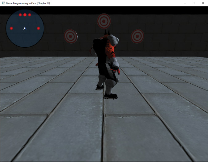
You now have everything in place to draw the first frame of an animation. Figure 12.5 shows the first frame of the CatActionIdle.gpanim animation. This and other animations in this chapter are also by Pior Oberson.
Updating Animations
The final step to get a working skeletal animation system is to update the animation every frame, based on delta time. You need to change the Animation class so that it correctly gets the pose based on the time in the animation, and you need to add an Update function to SkeletalMeshComponent.
For the GetGlobalPoseAtTime function, in Listing 12.11, you can no longer hard-code it to only use frame 0 of the animation. Instead, based on the duration of each frame and the current time, you figure out the frame before the current time (frame) and the frame after the current time (nextFrame). You then calculate a value from 0.0 to 1.0 that specifies where exactly between the two frames you are (pct). This way, you can account for the animation and game frame rates being different. Once you have this fractional value, you compute the global poses mostly the same as before. However, now instead of directly using a BoneTransform for a frame, you interpolate between the bone transforms of frame and nextFrame to figure out the correct in-between pose.
Listing 12.11 Final Version of GetGlobalPoseAtTime
void Animation::GetGlobalPoseAtTime(std::vector<Matrix4>& outPoses,
const Skeleton* inSkeleton, float inTime) const
{
if (outPoses.size() != mNumBones)
{
outPoses.resize(mNumBones);
}
// Figure out the current frame index and next frame
// (This assumes inTime is bounded by [0, AnimDuration]
size_t frame = static_cast<size_t>(inTime / mFrameDuration);
size_t nextFrame = frame + 1;
// Calculate fractional value between frame and next frame
float pct = inTime / mFrameDuration - frame;
// Setup the pose for the root
if (mTracks[0].size() > 0)
{
// Interpolate between the current frame's pose and the next frame
BoneTransform interp = BoneTransform::Interpolate(mTracks[0][frame],
mTracks[0][nextFrame], pct);
outPoses[0] = interp.ToMatrix();
}
else
{
outPoses[0] = Matrix4::Identity;
}
const std::vector<Skeleton::Bone>& bones = inSkeleton->GetBones();
// Now setup the poses for the rest
for (size_t bone = 1; bone < mNumBones; bone++)
{
Matrix4 localMat; // (Defaults to identity)
if (mTracks[bone].size() > 0)
{
BoneTransform interp =
BoneTransform::Interpolate(mTracks[bone][frame],
mTracks[bone][nextFrame], pct);
localMat = interp.ToMatrix();
}
outPoses[bone] = localMat * outPoses[bones[bone].mParent];
}
}
Then, in SkeletalMeshComponent, you add an Update function:
void SkeletalMeshComponent::Update(float deltaTime)
{
if (mAnimation && mSkeleton)
{
mAnimTime += deltaTime * mAnimPlayRate;
// Wrap around anim time if past duration
while (mAnimTime > mAnimation->GetDuration())
{ mAnimTime -= mAnimation->GetDuration(); }
// Recompute matrix palette
ComputeMatrixPalette();
}
}
Here, all you do is update mAnimTime based on delta time and the animation play rate. You also wrap mAnimTime around as the animation loops. This works correctly even when transitioning from the last frame of the animation to the first because, as mentioned earlier, the animation data duplicates the first frame at the end of the track.
Finally, Update calls ComputeMatrixPalette. This function uses GetGlobalPoseAtTime to calculate the new matrix palette for this frame.
Because SkeletalMeshComponent is a component, the owning actor calls Update every frame. Then in the “generate outputs” phase of the game loop, the SkeletalMeshComponent draws with this new matrix palette as usual, which means the animation now updates onscreen!
Game Project
This chapter’s game project implements skeletal animation as described in this chapter. It includes the SkeletalMeshComponent, Animation, and Skeleton classes, as well as the skinned vertex shader. The code is available in the book’s GitHub repository, in the Chapter12 directory. Open Chapter12-windows.sln in Windows and Chapter12-mac.xcodeproj on Mac.
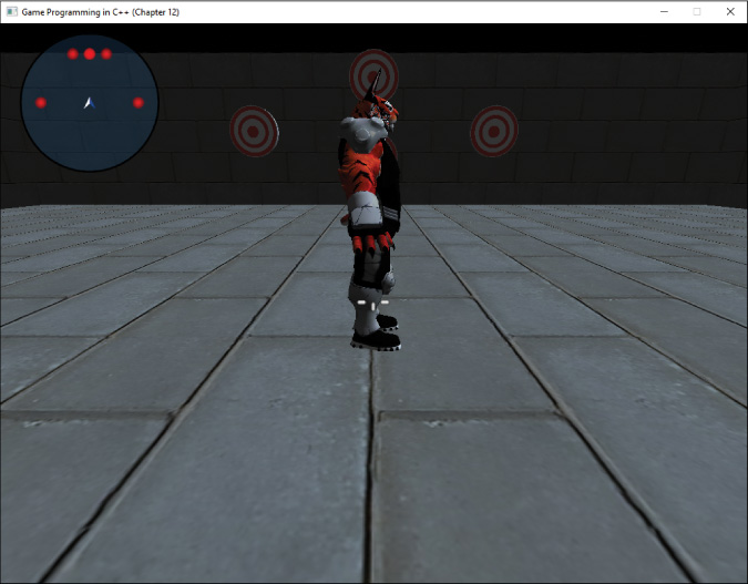
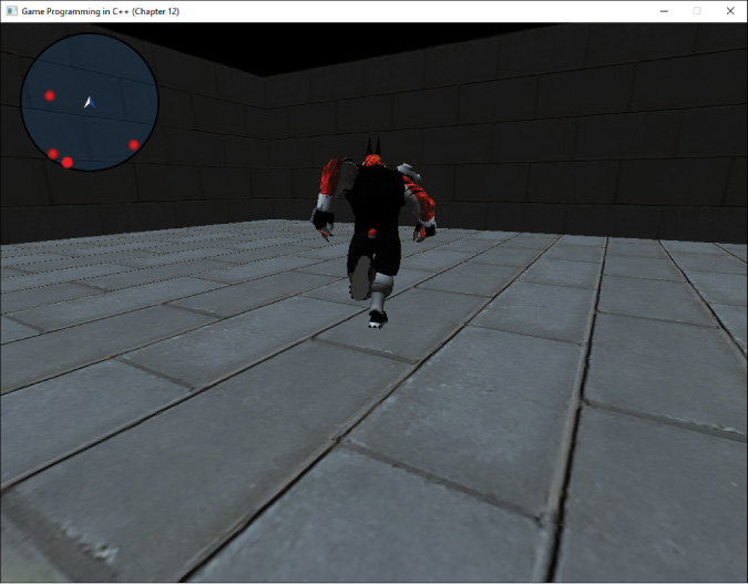
This chapter’s game project goes back to the follow camera discussed in Chapter 9, “Cameras,” to make the character visible. The FollowActor class has a SkeletalMeshComponent component, and it thus uses the animation code. The player can use the WASD keys to move the character around. When the character is standing still, an idle animation plays. When the player moves the character, a running animation plays (see Figure 12.6). Currently, the transition between the two animations is not smooth, but you will change that in Exercise 12.2.
Summary
This chapter provides a comprehensive overview of skeletal animation. In skeletal animation, a character has a rigid skeleton that animates, and vertices act like a skin that deforms with this skeleton. The skeleton contains a hierarchy of bones, and every bone except for the root has a parent bone.
The bind pose is the initial pose of the skeleton, prior to any animations. You can store a local transform for each bone in bind pose, which describes the position and orientation of a bone relative to its parent. A global transform instead describes the position and orientation of a bone relative to object space. You can convert a local transform into a global one by multiplying the local pose by the global pose of its parent. The root bone’s local pose and global pose are identical.
The inverse bind pose matrix is the inverse of each bone’s global bind pose matrix. This matrix transforms a point in object space while in bind pose into the bone’s coordinate space while in bind pose.
An animation is a sequence of poses played back over time. As with bind pose, you can construct a global pose matrix for the current pose for each bone. These current pose matrices can transform a point in a bone’s coordinate space while in bind pose into object space for the current pose.
The matrix palette stores the multiplication of the inverse bind pose matrix and the current pose matrix for each bone. When computing the object space position of a skinned vertex, you use the matrix palette entries for any bones that influence the vertex.
Additional Reading
Jason Gregory takes an in-depth look at more advanced topics in animation systems, such as blending animations, compressing animation data, and inverse kinematics.
Gregory, Jason. Game Engine Architecture, 2nd edition. Boca Raton: CRC Press, 2014.
Exercises
In this chapter’s exercises you will add features to the animation system. In Exercise 12.1 you add support for getting the position of a bone in the current pose, and in Exercise 12.2 you add blending when transitioning between two animations.
Exercise 12.1
It’s useful for a game to get the position of a bone as an animation plays. For example, if a character holds an object in his hand, you need to know the position of the bone as the animation changes. Otherwise, the character will no longer hold the item properly!
Because the SkeletalMeshComponent knows the progress in the animation, the code for this system needs to go in here. First, add as a member variable a std::vector to store the current pose matrices. Then, when the code calls GetGlobalPoseAtTime, save the current pose matrices in this member variable.
Next, add a function called GetBonePosition that takes the name of a bone and returns the object space position of the bone in the current pose. This is easier than it sounds because if you multiply a zero vector by the current pose matrix for a bone, you get the object space position of that bone in the current pose. This works because a zero vector here means it is exactly at the origin of the bone’s local space, and then the current pose matrix transforms it back to object space.
Exercise 12.2
Currently, SkeletalMeshComponent::PlayAnimation instantly switches to a new animation. This does not look very polished, and you can address this issue by adding blending to the animations. First, add an optional blend time parameter to PlayAnimation, which represents the duration of the blend. To blend between multiple animations, you must track each animation and animation time separately. If you limit blending to only two animations, you just need to duplicate those member variables.
Then, to blend between the animations, when you call GetGlobalPoseAtTime, you need to do so for both active animations. You need to get the bone transforms of every bone for each animation, interpolate these bone transforms to get the final transforms, and then convert these to the pose matrices to get the blended current pose.