
Chapter 5
Opengl
This chapter provides an in-depth introduction on how to use OpenGL for graphics in games. It covers many topics, including initializing OpenGL, using triangles, writing shader programs, using matrices for transforms, and adding support for textures. The game project for this chapter converts the game project from Chapter 3, “Vectors and Basic Physics,” to use OpenGL for all its graphics rendering.
Initializing OpenGL
Although the SDL renderer supports 2D graphics, it does not support 3D. Thus, to switch to 3D, which is used in every subsequent chapter in this book, you need to switch from SDL 2D graphics to a different library that supports both 2D and 3D graphics.
This book uses the OpenGL library. OpenGL is an industry-standard library for cross-platform 2D/3D graphics that’s been around for 25 years. Unsurprisingly, the library has been around so long that it has evolved in many ways over the years. The set of functions the original version of OpenGL used is very different from the set in modern OpenGL. This book uses functions defined up to and including OpenGL 3.3.
warning
OLDER VERSIONS OF OPENGL ARE VERY DIFFERENT: Be careful when consulting any online OpenGL references, as many refer to older versions of OpenGL.
The goal of this chapter is to convert the game project from Chapter 3 from SDL graphics to OpenGL graphics. You need to take a lot of steps to get there. This section walks through the steps of configuring and initializing OpenGL and a helper library called GLEW.
Setting Up the OpenGL Window
To use OpenGL, you must drop usage of the SDL_Renderer from the earlier chapters. You therefore need to remove all references to SDL_Renderer, including the mRenderer variable in Game, the call to SDL_CreateRenderer, and any calls to the SDL functions in GenerateOuput. This also means that the SpriteComponent code (which relies on SDL_Renderer) won’t work without changes. For now, all the code in Game::GenerateOutput is commented out until OpenGL is up and running.
In SDL, when you create a window, you can request a window for OpenGL usage by passing in the SDL_WINDOW_OPENGL flag as the final parameter of the SDL_CreateWindow call:
mWindow = SDL_CreateWindow("Game Programming in C++ (Chapter 5)", 100, 100,
1024, 768, SDL_WINDOW_OPENGL);
Prior to creating the OpenGL window, you can request attributes such as the version of OpenGL, the color depth, and several other parameters. To configure these parameters, you use the SDL_GL_SetAttribute function:
// Set OpenGL window's attributes (use prior to creating the window)
// Returns 0 if successful, otherwise a negative value
SDL_GL_SetAttribute(
SDL_GLattr attr, // Attribute to set
int value // Value for this attribute
);
There are several different attributes in the SDL_GLattr enum, but this chapter uses only some of them. To set the attributes, you add the code in Listing 5.1 prior to the call of SDL_CreateWindow inside Game::Initialize. This code sets several attributes. First, it requests the core OpenGL profile.
note
There are three main profiles supported by OpenGL: core, compatibility, and ES. The core profile is the recommended default profile for a desktop environment. The only difference between the core and compatibility profiles is that the compatibility profile allows the program to call OpenGL functions that are deprecated (no longer intended for use). The OpenGL ES profile is for mobile development.
Listing 5.1 Requesting OpenGL Attributes
// Use the core OpenGL profile
SDL_GL_SetAttribute(SDL_GL_CONTEXT_PROFILE_MASK,
SDL_GL_CONTEXT_PROFILE_CORE);
// Specify version 3.3
SDL_GL_SetAttribute(SDL_GL_CONTEXT_MAJOR_VERSION, 3);
SDL_GL_SetAttribute(SDL_GL_CONTEXT_MINOR_VERSION, 3);
// Request a color buffer with 8-bits per RGBA channel
SDL_GL_SetAttribute(SDL_GL_RED_SIZE, 8);
SDL_GL_SetAttribute(SDL_GL_GREEN_SIZE, 8);
SDL_GL_SetAttribute(SDL_GL_BLUE_SIZE, 8);
SDL_GL_SetAttribute(SDL_GL_ALPHA_SIZE, 8);
// Enable double buffering
SDL_GL_SetAttribute(SDL_GL_DOUBLEBUFFER, 1);
// Force OpenGL to use hardware acceleration
SDL_GL_SetAttribute(SDL_GL_ACCELERATED_VISUAL, 1);
The next two attributes request OpenGL version 3.3. Although there are newer versions of OpenGL, the 3.3 version supports all the required features for this book and has a feature set closely aligned with the ES profile. Thus, most of the code in this book should also work on current mobile devices.
The next attributes specify the bit depth of each channel. In this case, the program requests 8 bits per RGBA channel, for a total of 32 bits per pixel. The second-to-last attribute asks to enable double buffering. The final attribute asks to run OpenGL with hardware acceleration. This means that the OpenGL rendering will run on graphics hardware (a GPU).
The OpenGL Context and Initializing GLEW
Once the OpenGL attributes are set and you’ve created the window, the next step is to create an OpenGL context. Think of a context as the “world” of OpenGL that contains every item that OpenGL knows about, such as the color buffer, any images or models loaded, and any other OpenGL objects. (While it is possible to have multiple contexts in one OpenGL program, this book sticks to one.)
To create the context, first add the following member variable to Game:
SDL_GLContext mContext;
Next, immediately after creating the SDL window with SDL_CreateWindow, add the following line of code, which creates an OpenGL context and saves it in the member variable:
mContext = SDL_GL_CreateContext(mWindow);
As with creating and deleting the window, you need to delete the OpenGL context in the destructor. To do this, add the following line of code to Game::Shutdown, right before the call to SDL_DeleteWindow:
SDL_GL_DeleteContext(mContext);
Although the program now creates an OpenGL context, there is one final hurdle you must pass to gain access to the full set of OpenGL 3.3 features. OpenGL supports backward compatibility with an extension system. Normally, you must query any extensions you want manually, which is tedious. To simplify this process, you can use an open source library called the OpenGL Extension Wrangler Library (GLEW). With one simple function call, GLEW automatically initializes all extension functions supported by the current OpenGL context’s version. So in this case, GLEW initializes all extension functions supported by OpenGL 3.3 and earlier.
To initialize GLEW, you add the following code immediately after creating the OpenGL context:
// Initialize GLEW
glewExperimental = GL_TRUE;
if (glewInit() != GLEW_OK)
{
SDL_Log("Failed to initialize GLEW.");
return false;
}
// On some platforms, GLEW will emit a benign error code,
// so clear it
glGetError();
The glewExperimental line prevents an initialization error that may occur when using the core context on some platforms. Furthermore, because some platforms emit a benign error code when initializing GLEW, the call to glGetError clears this error code.
note
Some old PC machines with integrated graphics (from 2012 or earlier) may have issues running OpenGL version 3.3. In this case, you can try two things: updating to newer graphics drivers or requesting OpenGL version 3.1.
Rendering a Frame
You now need to convert the clear, draw scene, and swap buffers process in Game::GenerateOutput to use OpenGL functions:
// Set the clear color to gray
glClearColor(0.86f, 0.86f, 0.86f, 1.0f);
// Clear the color buffer
glClear(GL_COLOR_BUFFER_BIT);
// TODO: Draw the scene
// Swap the buffers, which also displays the scene
SDL_GL_SwapWindow(mWindow);
This code first sets the clear color to 86% red, 86% green, 86% blue, and 100% alpha, which yields a gray color. The glClear call with the GL_COLOR_BUFFER_BIT parameter clears the color buffer to the specified color. Finally, the SDL_GL_SwapWindow call swaps the front buffer and back buffer. At this point, running the game yields a gray screen because you aren’t drawing the SpriteComponents yet.
Triangle Basics
The graphical needs of 2D and 3D games couldn’t seem more different. As discussed in Chapter 2, “Game Objects and 2D Graphics,” most 2D games use sprites for their 2D characters. On the other hand, a 3D game features a simulated 3D environment that you somehow flatten into a 2D image that you show onscreen.
Early 2D games could simply copy sprite images into the desired locations of the color buffer. This process, called blitting, was efficient on sprite-based consoles such as the Nintendo Entertainment System (NES). However, modern graphical hardware is inefficient at blitting but is very efficient at polygonal rendering. Because of this, nearly all modern games, whether 2D or 3D, ultimately use polygons for their graphical needs.
Why Polygons?
There are many ways a computer could simulate a 3D environment. Polygons are popular in games for a multitude of reasons. Compared to other 3D graphics techniques, polygons do not require as many calculations at runtime. Furthermore, polygons are scalable: A game running on less-powerful hardware could simply use 3D models with fewer polygons. And, importantly, you can represent most 3D objects with polygons.
Triangles are the polygon of choice for most games. Triangles are the simplest polygon, and you need only three points (or vertices) to create a triangle. Furthermore, a triangle can only lie on a single plane. In other words, the three points of a triangle must be coplanar. Finally, triangles tessellate easily, meaning it’s relatively simple to break any complex 3D object into many triangles. The remainder of this chapter talks about triangles, but the techniques discussed here also work for other polygons (such as quads), provided that they maintain the coplanar property.
2D games use triangles to represent sprites by drawing a rectangle and filling in the rectangle with colors from an image file. We discuss this in much greater detail later in the chapter.
Normalized Device Coordinates
To draw a triangle, you must specify the coordinates of its three vertices. Recall that in SDL, the top-left corner of the screen is (0, 0), positive x is to the right, and positive y is down. More generally, a coordinate space specifies where the origin is and in which direction its coordinates increase. The basis vectors of the coordinate space are the direction in which the coordinates increase.
An example of a coordinate space from basic geometry is a Cartesian coordinate system (see Figure 5.1). In a 2D Cartesian coordinate system, the origin (0, 0) has a specific point (usually the center), positive x is to the right, and positive y is up.

Normalized device coordinates (NDC) is the default coordinate system used with OpenGL. Given an OpenGL window, the center of the window is the origin in normalized device coordinates. Furthermore, the bottom-left corner is (–1, –1), and the top-right corner is (1, 1). This is regardless of the width and height of the window (hence normalized device coordinates). Internally, the graphics hardware then converts these NDC into the corresponding pixels in the window.
For example, to draw a square with sides of unit length in the center of the window, you need two triangles. The first triangle has the vertices (–0.5, 0.5), (0.5, 0.5), and (0.5, –0.5), and the second triangle has the vertices (0.5, –0.5), (–0.5, –0.5), and (–0.5, 0.5). Figure 5.2 illustrates this square. Keep in mind that if the length and width of the window are not uniform, a square in normalized device coordinates will not look like a square onscreen.

In 3D, the z component of normalized device coordinates also ranges from [–1, 1], with a positive z value going into the screen. For now, we stick with a z value of zero. We’ll explore 3D in much greater detail in Chapter 6, “3D Graphics.”
Vertex and Index Buffers
Suppose you have a 3D model comprised of many triangles. You need some way to store the vertices of these triangles in memory. The simplest approach is to directly store the coordinates of each triangle in a contiguous array or buffer. For example, assuming 3D coordinates, the following array contains the vertices of the two triangles shown in Figure 5.2:
float vertices[] = {
-0.5f, 0.5f, 0.0f,
0.5f, 0.5f, 0.0f,
0.5f, -0.5f, 0.0f,
0.5f, -0.5f, 0.0f,
-0.5f, -0.5f, 0.0f,
-0.5f, 0.5f, 0.0f,
};
Even in this simple example, the array of vertices has some duplicate data. Specifically, the coordinates (–0.5, 0.5, 0.0) and (0.5, –0.5, 0.0) appear twice. If there were a way to remove these duplicates, you would cut the number of values stored in the buffer by 33%. Rather than having 12 values, you would have only 8. Assuming single-precision floats that use 4 bytes each, you’d save 24 bytes of memory by removing the duplicates. This might seem insignificant, but imagine a much larger model with 20,000 triangles. In this case, the amount of memory wasted due to duplicate coordinates would be high.
The solution to this issue has two parts. First, you create a vertex buffer that contains only the unique coordinates used by the 3D geometry. Then, to specify the vertices of each triangle, you index into this vertex buffer (much like indexing into an array). The aptly named index buffer contains the indices for each individual triangle, in sets of three. For this example’s sample square, you’d need the following vertex and index buffers:
float vertexBuffer[] = {
-0.5f, 0.5f, 0.0f, // vertex 0
0.5f, 0.5f, 0.0f, // vertex 1
0.5f, -0.5f, 0.0f, // vertex 2
-0.5f, -0.5f, 0.0f // vertex 3
};
unsigned short indexBuffer[] = {
0, 1, 2,
2, 3, 0
};
For example, the first triangle has the vertices 0, 1, and 2, which corresponds to the coordinates (–0.5, 0.5, 0.0), (0.5, 0.5, 0.0), and (0.5, –0.5, 0.0). Keep in mind that the index is the vertex number, not the floating-point element (for example, vertex 1 instead of “index 2” of the array). Also note that this code uses an unsigned short (typically 16 bits) for the index buffer, which reduces the memory footprint of the index buffer. You can use smaller bit size integers to save memory in the index buffer.
In this example, the vertex/index buffer combination uses 12 × 4 + 6 × 2, or 60 total bytes. On the other hand, if you just used the original vertices, you’d need 72 bytes. While the savings in this example is only 20%, a more complex model would save much more memory by using the vertex/index buffer combination.
To use the vertex and index buffers, you must let OpenGL know about them. OpenGL uses a vertex array object to encapsulate a vertex buffer, an index buffer, and the vertex layout. The vertex layout specifies what data you store for each vertex in the model. For now, assume the vertex layout is a 3D position (you can just use a z component of 0.0f if you want something 2D). Later in this chapter you’ll add other data to each vertex.
Because any model needs a vertex array object, it makes sense to encapsulate its behavior in a VertexArray class. Listing 5.2 shows the declaration of this class.
Listing 5.2 VertexArray Declaration
class VertexArray
{
public:
VertexArray(const float* verts, unsigned int numVerts,
const unsigned int* indices, unsigned int numIndices);
~VertexArray();
// Activate this vertex array (so we can draw it)
void SetActive();
unsigned int GetNumIndices() const { return mNumIndices; }
unsigned int GetNumVerts() const { return mNumVerts; }
private:
// How many vertices in the vertex buffer?
unsigned int mNumVerts;
// How many indices in the index buffer
unsigned int mNumIndices;
// OpenGL ID of the vertex buffer
unsigned int mVertexBuffer;
// OpenGL ID of the index buffer
unsigned int mIndexBuffer;
// OpenGL ID of the vertex array object
unsigned int mVertexArray;
};
The constructor for VertexArray takes in pointers to the vertex and index buffer arrays so that it can hand off the data to OpenGL (which will ultimately load the data on the graphics hardware). Note that the member data contains several unsigned integers for the vertex buffer, index buffer, and vertex array object. This is because OpenGL does not return pointers to objects that it creates. Instead, you merely get back an integral ID number. Keep in mind that the ID numbers are not unique across different types of objects. It’s therefore very possible to have an ID of 1 for both the vertex and index buffers because OpenGL considers them different types of objects.
The implementation of the VertexArray constructor is complex. First, create the vertex array object and store its ID in the mVertexArray member variable:
glGenVertexArrays(1, &mVertexArray);
glBindVertexArray(mVertexArray);
Once you have a vertex array object, you can create a vertex buffer:
glGenBuffers(1, &mVertexBuffer);
glBindBuffer(GL_ARRAY_BUFFER, mVertexBuffer);
The GL_ARRAY_BUFFER parameter to glBindBuffer means that you intend to use the buffer as a vertex buffer.
Once you have a vertex buffer, you need to copy the verts data passed into the VertexArray constructor into this vertex buffer. To copy the data, use glBufferData, which takes several parameters:
glBufferData(
GL_ARRAY_BUFFER, // The active buffer type to write to
numVerts * 3 * sizeof(float), // Number of bytes to copy
verts, // Source to copy from (pointer)
GL_STATIC_DRAW // How will we use this data?
);
Note that you don’t pass in the object ID to glBufferData; instead, you specify a currently bound buffer type to write to. In this case, GL_ARRAY_BUFFER means use the vertex buffer just created.
For the second parameter, you pass in the number of bytes, which is the amount of data for each vertex multiplied by the number of vertices. For now, you can assume that each vertex contains three floats for (x, y, z).
The usage parameter specifies how you want to use the buffer data. A GL_STATIC_DRAW usage means you only want to load the data once and use it frequently for drawing.
Next, create an index buffer. This is very similar to creating the vertex buffer, except you instead specify the GL_ELEMENT_ARRAY_BUFFER type, which corresponds to an index buffer:
glGenBuffers(1, &mIndexBuffer);
glBindBuffer(GL_ELEMENT_ARRAY_BUFFER, mIndexBuffer);
Then copy the indices data into the index buffer:
glBufferData(
GL_ELEMENT_ARRAY_BUFFER, // Index buffer
numIndices * sizeof(unsigned int), // Size of data
indices, GL_STATIC_DRAW);
Note that the type here is GL_ELEMENT_ARRAY_BUFFER, and the size is the number of indices multiplied by an unsigned int because that’s the type used for indices here.
Finally, you must specify a vertex layout, also called the vertex attributes. As mentioned earlier, the current layout is a position with three float values.
To enable the first vertex attribute (attribute 0), use glEnableVertexAttribArray:
glEnableVertexAttribArray(0);
You then use glVertexAttribPointer to specify the size, type, and format of the attribute:
glVertexAttribPointer(
0, // Attribute index (0 for first one)
3, // Number of components (3 in this case)
GL_FLOAT, // Type of the components
GL_FALSE, // (Only used for integral types)
sizeof(float) * 3, // Stride (usually size of each vertex)
0 // Offset from start of vertex to this attribute
);
The first two parameters are 0 and 3 because the position is attribute 0 of the vertex, and there are three components (x, y, z). Because each component is a float, you specify the GL_FLOAT type. The fourth parameter is only relevant for integral types, so here you set it to GL_FALSE. Finally, the stride is the byte offset between consecutive vertices’ attributes. But assuming you don’t have padding in the vertex buffer (which you usually don’t), the stride is just the size of the vertex. Finally, the offset is 0 because this is the only attribute. For additional attributes, you have to pass in a nonzero value for the offset.
The VertexArray’s destructor destroys the vertex buffer, index buffer, and vertex array object:
VertexArray::~VertexArray()
{
glDeleteBuffers(1, &mVertexBuffer);
glDeleteBuffers(1, &mIndexBuffer);
glDeleteVertexArrays(1, &mVertexArray);
}
Finally, the SetActive function calls glBindVertexArray, which just specifies which vertex array you’re currently using:.
void VertexArray::SetActive()
{
glBindVertexArray(mVertexArray);
}
The following code in Game::InitSpriteVerts allocates an instance of VertexArray and saves it in a member variable of Game called mSpriteVerts:
mSpriteVerts = new VertexArray(vertexBuffer, 4, indexBuffer, 6);
The vertex and index buffer variables here are the arrays for the sprite quad. In this case, there are 4 vertices in the vertex buffer and 6 indices in the index buffer (corresponding to the 2 triangles in the quad). You will use this member variable later in this chapter to draw sprites, as all sprites will ultimately use the same vertices.
Shaders
In a modern graphics pipeline, you don’t simply feed in the vertex/index buffers and have triangles draw. Instead, you specify how you want to draw the vertices. For example, should the triangles be a fixed color, or should they use a color from a texture? Do you want to perform lighting calculations for every pixel you draw?
Because there are many techniques you may want to use to display the scene, there is no truly one-size-fits-all method. To allow for more customization, graphics APIs including OpenGL support shader programs—small programs that execute on the graphics hardware to perform specific tasks. Importantly, shaders are separate programs, with their own separate main functions.
note
Shader programs do not use the C++ programming language. This book uses the GLSL programming language for shader programs. Although GLSL superficially looks like C, there are many semantics specific to GLSL. Rather than present all the details of GLSL at once, this book introduces the concepts as needed.
Because shaders are separate programs, you write them in separate files. Then in your C++ code, you need to tell OpenGL when to compile and load these shader programs and specify what you want OpenGL to use these shader programs for.
Although you can use several different types of shaders in games, this book focuses on the two most important ones: the vertex shader and the fragment (or pixel) shader.
Vertex Shaders
A vertex shader program runs once for every vertex of every triangle drawn. The vertex shader receives the vertex attribute data as an input. The vertex shader can then modify these vertex attributes as it sees fit. While it may seem unclear why you’d want to modify vertex attributes, it’ll become more apparent as this chapter continues.
Given that triangles have three vertices, you can think of a vertex shader as running three times per triangle. However, if you use vertex and index buffers, then you will invoke the vertex shader less often because some triangles share vertices. This is an additional advantage of using a vertex and index buffer instead just a vertex buffer. Note that if you draw the same model multiple times per frame, the vertex shader calls for each time you draw it are independent of each other.
Fragment Shaders
After the vertices of a triangle have gone through the vertex shader, OpenGL must determine which pixels in the color buffer correspond to the triangle. This process of converting the triangle into pixels is rasterization. There are many different rasterization algorithms, but today’s graphics hardware does rasterization for us.
The job of a fragment shader (or pixel shader) is to determine the color of each pixel, and so the fragment shader program executes at least once for every pixel. This color may take into account properties of the surface, such as textures, colors, and materials. If the scene has any lighting, the fragment shader might also do lighting calculations. Because there are so many potential calculations, the average 3D game has a lot more code in the fragment shader than in the vertex shader.
Writing Basic Shaders
Although you could load in the shader programs from hard-coded strings in C++ code, it’s much better to put them in separate files. This book uses the .vert extension for vertex shader files and the .frag extension for fragment shader files.
Because these source files are in a different programming language, they are in the Shaders subdirectory for the chapter. For example, Chapter05/Shaders contains the source files for the shaders in this chapter.
The Basic.vert File
Basic.vert contains the vertex shader code. Remember that this code is not C++ code.
Every GLSL shader file first must specify the version of the GLSL programming language used. The following line represents the version of GLSL corresponding to OpenGL 3.3:
#version 330
Next, because this is a vertex shader, you must specify the vertex attributes for each vertex. These attributes should match the attributes of the vertex array object created earlier, and are the input to the vertex shader. However, in GLSL the main function does not receive any parameters. Instead, the shader inputs look like global variables, marked with a special in keyword.
For now, you only have one input variable—the 3D position. The following line declares this input variable:
in vec3 inPosition;
The type of inPosition variable is vec3, which corresponds to a vector of three floating-point values. This will contain the x, y, and z components corresponding to the vertex’s position. You can access each component of the vec3 via dot syntax; for example, inPosition.x accesses the x component of the vector.
As with a C/C++ program, a shader program has a main function as its entry point:
void main()
{
// TODO: Shader code goes here
}
Note that the main function here returns void. GLSL also uses global variables to define the outputs of the shader. In this case, you’ll use a built-in variable called gl_Position to store the vertex position output of the shader.
For now, the vertex shader directly copies the vertex position from inPosition to gl_Position. However, gl_Position expects four components: the normal (x, y, z) coordinates plus a fourth component called the w component. We’ll look at what this w represents later in this chapter. For now, assume that w is always 1.0. To convert inPosition from vec3 to vec4, you can use the following syntax:
gl_Position = vec4(inPosition, 1.0);
Listing 5.3 shows the complete Basic.vert code, which simply copies along the vertex position without any modification.
// Request GLSL 3.3
#version 330
// Any vertex attributes go here
// For now, just a position.
in vec3 inPosition;
void main()
{
// Directly pass along inPosition to gl_Position
gl_Position = vec4(inPosition, 1.0);
}
The Basic.frag File
The job of the fragment shader is to compute an output color for the current pixel. For Basic.frag, you’ll hard-code a blue output color for all pixels.
As with the vertex shader, the fragment shader always begin with a #version line. Next, you declare a global variable to store the output color, using the out variable specifier:
out vec4 outColor;
The outColor variable is a vec4 corresponding to the four components of the RGBA color buffer.
Next, you declare the entry point of the fragment shader program. Inside this function, you set outColor to the desired color for the pixel. The RGBA value of blue is (0.0, 0.0, 1.0, 1.0), which means you use the following assignment:
outColor = vec4(0.0, 0.0, 1.0, 1.0);
Listing 5.4 gives the full source code for Basic.frag.
// Request GLSL 3.3
#version 330
// This is output color to the color buffer
out vec4 outColor;
void main()
{
// Set to blue
outColor = vec4(0.0, 0.0, 1.0, 1.0);
}
Loading Shaders
Once you have the separate shader files written, you must load in these shaders in the game’s C++ code to let OpenGL know about them. At a high level, you need to follow these steps:
1. Load and compile the vertex shader.
2. Load and compile the fragment shader.
3. Link the two shaders together into a “shader program.”
There are many steps to loading a shader, so it is a good idea to declare a separate Shader class, as in Listing 5.5.
Listing 5.5 Initial Shader Declaration
class Shader
{
public:
Shader();
~Shader();
// Load the vertex/fragment shaders with the given names
bool Load(const std::string& vertName,
const std::string& fragName);
// Set this as the active shader program
void SetActive();
private:
// Tries to compile the specified shader
bool CompileShader(const std::string& fileName,
GLenum shaderType, GLuint& outShader);
// Tests whether shader compiled successfully
bool IsCompiled(GLuint shader);
// Tests whether vertex/fragment programs link
bool IsValidProgram();
// Store the shader object IDs
GLuint mVertexShader;
GLuint mFragShader;
GLuint mShaderProgram;
};
Note how the member variables here correspond to shader object IDs. They have object IDs much like the vertex and index buffers. (GLuint is simply OpenGL’s version of unsigned int.)
You declare CompileShader, IsCompiled, and IsValidProgram in the private section because they are helper functions used by Load. This reduces the code duplication in Load.
The CompileShader Function
CompileShader takes three parameters: the name of the shader file to compile, the type of shader, and a reference parameter to store the ID of the shader. The return value is a bool that denotes whether CompileShader succeeded.
Listing 5.6 shows the implementation of CompileShader, which has several steps. First, create an ifstream to load in the file. Next, use a string stream to load the entire contents of the file into a single string, contents, and get the C-style string pointer with the c_str function.
Next, the glCreateShader function call creates an OpenGL shader object corresponding to the shader (and saves this ID in outShader). The shaderType parameter can be GL_VERTEX_SHADER, GL_FRAGMENT_SHADER, or a few other shader types.
The glShaderSource call specifies the string containing the shader source code, and glCompileShader compiles the code. You then use the IsCompiled helper function (implemented in a moment) to validate that the shader compiles.
In the event of any errors, including being unable to load the shader file or failing to compile it, CompileShader outputs an error message and returns false.
Listing 5.6 Shader::CompileShader Implementation
bool Shader::CompileShader(const std::string& fileName,
GLenum shaderType,
GLuint& outShader)
{
// Open file
std::ifstream shaderFile(fileName);
if (shaderFile.is_open())
{
// Read all the text into a string
std::stringstream sstream;
sstream << shaderFile.rdbuf();
std::string contents = sstream.str();
const char* contentsChar = contents.c_str();
// Create a shader of the specified type
outShader = glCreateShader(shaderType);
// Set the source characters and try to compile
glShaderSource(outShader, 1, &(contentsChar), nullptr);
glCompileShader(outShader);
if (!IsCompiled(outShader))
{
SDL_Log("Failed to compile shader %s", fileName.c_str());
return false;
}
}
else
{
SDL_Log("Shader file not found: %s", fileName.c_str());
return false;
}
return true;
}
The IsCompiled Function
The IsCompiled function, shown in Listing 5.7, validates whether a shader object compiled, and if it didn’t, it outputs the compilation error message. This way, you can get some information about why a shader fails to compile.
Listing 5.7 Shader::IsCompiled Implementation
bool Shader::IsCompiled(GLuint shader)
{
GLint status;
// Query the compile status
glGetShaderiv(shader, GL_COMPILE_STATUS, &status);
if (status != GL_TRUE)
{
char buffer[512];
memset(buffer, 0, 512);
glGetShaderInfoLog(shader, 511, nullptr, buffer);
SDL_Log("GLSL Compile Failed:
%s", buffer);
return false;
}
return true;
}
The glGetShaderiv function queries the compilation status, which the function returns as an integral status code. If this status is not GL_TRUE, there was an error. In the event of an error, you can get a human-readable compile error message with glGetShaderInfoLog.
The Load Function
The Load function in Listing 5.8 takes in the filenames of both the vertex and fragment shaders and then tries to compile and link these shaders together.
As shown in Listing 5.8, you compile both the vertex and fragment shaders using CompileShader and then save their objects IDs in mVertexShader and mFragShader, respectively. If either of the CompileShader calls fail, Load returns false.
Listing 5.8 Shader::Load Implementation
bool Shader::Load(const std::string& vertName,
const std::string& fragName)
{
// Compile vertex and fragment shaders
if (!CompileShader(vertName, GL_VERTEX_SHADER, mVertexShader) ||
!CompileShader(fragName, GL_FRAGMENT_SHADER, mFragShader))
{
return false;
}
// Now create a shader program that
// links together the vertex/frag shaders
mShaderProgram = glCreateProgram();
glAttachShader(mShaderProgram, mVertexShader);
glAttachShader(mShaderProgram, mFragShader);
glLinkProgram(mShaderProgram);
// Verify that the program linked successfully
if (!IsValidProgram())
{
return false;
}
return true;
}
After you’ve compiled both the fragment and vertex shader, you link them together in a third object, called a shader program. When it’s time to draw an object, OpenGL uses the currently active shader program to render the triangles.
You create a shader program with glCreateProgram, which returns the object ID to the new shader program. Next, use glAttachShader to add the vertex and fragment shaders to the combined shader program. Then use glLinkProgram to link together all attached shaders into the final shader program.
As with shader compilation, figuring out whether the link was successful requires additional function calls, which you can place in the IsValidProgram helper function.
The IsValidProgram Function
The code for IsValidProgram is very similar to the code for IsCompiled. There are only two differences. First, instead of calling glGetShaderiv, call glGetProgramiv:
glGetProgramiv(mShaderProgram, GL_LINK_STATUS, &status);
Next, instead of calling glGetShaderInfoLog, call glGetProgramInfoLog:
glGetProgramInfoLog(mShaderProgram, 511, nullptr, buffer);
The SetActive Function
The SetActive function sets a shader program as the active one:
void Shader::SetActive()
{
glUseProgram(mShaderProgram);
}
OpenGL uses the active shader when drawing triangles.
The Unload Function
The Unload function simply deletes the shader program, the vertex shader, and the pixel shader:
void Shader::Unload()
{
glDeleteProgram(mShaderProgram);
glDeleteShader(mVertexShader);
glDeleteShader(mFragShader);
}
Adding a Shader to the Game
With the Shader class, you can now add a Shader pointer as a member variable to Game:
class Shader* mSpriteShader;
This variable is called mSpriteShader because, ultimately, you’ll use it to draw sprites. The LoadShaders function loads in the shader files and sets the shader as active:
bool Game::LoadShaders()
{
mSpriteShader = new Shader();
if (!mSpriteShader->Load("Shaders/Basic.vert", "Shaders/Basic.frag"))
{
return false;
}
mSpriteShader->SetActive();
}
You call LoadShaders in Game::Initialize immediately after finishing initialization of OpenGL and GLEW (and before you create the mSpriteVerts vertex array object).
After you’ve created simple vertex and pixel shaders and loaded in triangles, you can finally try to draw some triangles.
Drawing Triangles
As mentioned earlier, you can draw sprites with triangles by drawing rectangles onscreen. You’ve already loaded in the unit square vertices and a basic shader that can draw blue pixels. As before, you want to draw sprites in the Draw function in SpriteComponent.
First, you change the declaration of SpriteComponent::Draw so that it takes in Shader* instead of SDL_Renderer*. Next, draw a quad with a call to glDrawElements:
void SpriteComponent::Draw(Shader* shader)
{
glDrawElements(
GL_TRIANGLES, // Type of polygon/primitive to draw
6, // Number of indices in index buffer
GL_UNSIGNED_INT, // Type of each index
nullptr // Usually nullptr
);
}
The first parameter to glDrawElements specifies the type of element you’re drawing (in this case, triangles). The second parameter is the number of indices in the index buffer; in this case, because the index buffer for the unit square has six elements, you pass in 6 as the parameter. The third parameter is the type of each index, established earlier as unsigned int. The last parameter is nullptr.
The glDrawElements call requires both an active vertex array object and an active shader. On every frame, you need to activate both the sprite vertex array object and shader before drawing any SpriteComponents. You do this in the Game::GenerateOutput function, as shown in Listing 5.9. Once you’ve set the shader and vertex array as active, you call Draw once for each sprite in the scene.
Listing 5.9 Game::GenerateOutput Attempting to Draw Sprites
void Game::GenerateOutput()
{
// Set the clear color to gray
glClearColor(0.86f, 0.86f, 0.86f, 1.0f);
// Clear the color buffer
glClear(GL_COLOR_BUFFER_BIT);
// Set sprite shader and vertex array objects active
mSpriteShader ->SetActive();
mSpriteVerts ->SetActive();
// Draw all sprites
for (auto sprite : mSprites)
{
sprite ->Draw(mSpriteShader);
}
// Swap the buffers
SDL_GL_SwapWindow(mWindow);
return true;
}
What happens when you run this code now? Well, first, the fragment shader only writes out a blue color. So it’s reasonable to expect that you’d see blue squares for each SpriteComponent. However, there’s another issue: For every sprite, you use the same sprite verts. These sprite verts define a unit square in normalized device coordinates. This means that for every SpriteComponent, you merely draw the same unit square in NDC. Thus, if you run the game right now, you’ll see only a gray background and a rectangle, as in Figure 5.3.

It may seem like the solution is to define different vertex arrays for each sprite. However, it turns out that with only this one vertex array, you can draw whichever sprites you want to. The key is to take advantage the vertex shader’s ability to transform vertex attributes.
Transformation Basics
Suppose a game has 10 asteroids moving around. You could represent these 10 asteroids individually with different vertex array objects. However, you need these asteroids to show up in different locations onscreen. This means the triangles you draw for each asteroid need different normalized device coordinates.
A naïve idea is to create 10 different vertex buffers, 1 for each of the 10 asteroids, and recompute the vertex positions in these vertex buffers as needed. But this is wasteful both in terms of memory usage and in terms of computation. Changing vertices in vertex buffers and resubmitting them to OpenGL is not efficient.
Instead, think of a sprite in an abstract sense. Every sprite is ultimately just a rectangle. Different sprites may have different locations on the screen, different sizes, or different rotations, but they’re still rectangles.
Thinking of it this way, a more efficient solution is to have a single vertex buffer for the rectangle and just reuse it. Every time you draw the rectangle, you may have a position offset, scale, or rotation. But given the NDC unit square, you can change, or transform, it such that it is an arbitrary rectangle with an arbitrary position, scale, and/or orientation.
This same concept of reusing a single vertex buffer for a type of object also extends to 3D. For example, a game taking place in the forest might have hundreds of trees, many of which are only slight variations of each other. It’s inefficient to have a separate vertex buffer for every single instance of the same tree. Instead, you could create a single tree vertex buffer, and the game could draw many instances of this same tree with some variation in position, scale, and orientation.
Object Space
When you create a 3D object (such as in a 3D modeling program), you generally don’t express vertex positions in normalized device coordinates. Instead, the positions are relative to an arbitrary origin of the object itself. This origin is often in the center of the object, but it does not have to be. This coordinate space relative to the object itself is object space, or model space.
As discussed earlier in this chapter, defining a coordinate space requires knowing both the origin of the coordinate space and the direction in which the various components increase (the basis vectors). For example, some 3D modeling programs use +y as up, whereas others use +z as up. These different basis vectors define different object spaces for the objects. Figure 5.4 illustrates a 2D square where the center of the square is its object space origin, +y moves up, and +x moves right.

Now imagine a game that takes place in an office building. You’d need models for computer monitors, keyboards, desks, office chairs, and so on. You’d create each of these individual models in its own object space, which means each object’s vertex positions are relative to that model’s unique object space origin.
At runtime, you load each unique model into its own vertex array object (VAO). For example, you might have a VAO for the monitor, one for the keyboard, and so on. When it’s time to render the scene, each vertex of each object you draw goes to the vertex shader. If you just directly passed along the vertex positions, as in Basic.vert, then you’re saying that these vertex positions are in normalized device coordinates.
This is a problem because the coordinates for the models are not in NDC but instead are relative to each object’s unique object space. Passing through the vertex positions as is would yield garbage output.
World Space
To solve the problem with different objects having different object space coordinates, you first define a coordinate space for the game world itself. This coordinate space, called world space, has its own origin and basis vectors. For the game in the office building, the origin of world space might be in the center of the building on the ground floor.
Much as an office planner might place the desks and chairs at different positions and orientations in the office, you can think of the objects in the game as having arbitrary positions, scales, or orientations relative to the world space origin. For example, if there are five instances of the same desk placed in the office, each of these instances needs information describing how the object appears in world space.
When you draw each instance of the desk, you use the same vertex array object for each desk. However, each instance now needs some additional information, specifying how you want to transform the object space coordinates into world space. You can send this extra data to the vertex shader when drawing an instance, which allows the vertex shader to adjust the vertex positions as needed. Of course, the graphics hardware ultimately needs the coordinates in NDC to draw them, so you still have an additional step after transforming the vertices into world space. For now, let’s look at how to transform vertices from their object space into world space.
Transforming to World Space
When transforming between coordinate spaces, you need to know whether the basis vectors between the two coordinate spaces are the same. For example, consider the point (0, 5) in object space. If you define object space with +y as up, this means that the point (0, 5) is five units “above” the origin. However, if you choose to define world space such that +y is to the right, (0, 5) is instead five units to the right.
For now, assume that the basis vectors in object and world space are the same. Because the game currently is 2D, you can assume that +y is up and +x is to the right for both object space and world space.
note
The 2D coordinate system used here is different from the SDL coordinate system where +y is down! This means the code for Actor::GetForward no longer negates the y component. Furthermore, if you use atan2 for any calculations, you no longer negate the first parameter.
Now consider a unit square centered around the object space origin, as in Figure 5.4. Assume that the world space origin is the center of the game window. The goal is to take the unit square centered around its object space origin and express it as a rectangle with an arbitrary position, scale, or orientation relative to the world space origin.
For example, suppose one instance of the rectangle should appear in world space such that it’s double in size and is 50 units to the right of the world space origin. You can accomplish this by applying mathematical operations to each vertex of the rectangle.
One approach is to use algebra equations to compute the correct vertex positions. Although you ultimately won’t approach it in this manner, this is a useful bridge to understanding the preferred solution. This chapter focuses on 2D coordinate systems, though the same method outlined here would also work in 3D (just with an additional z component).
Translation
Translation takes a point and translates, or moves, it by an offset. Given the point (x, y), you can translate it by the offset (a, b) by using the following equations:
![]()
For example, you could translate the point (1, 3) by the offset (20, 15) as follows:
![]()
If you apply the same translation to every vertex of a triangle, you translate the entire triangle.
Scale
When applied to each vertex in a triangle, scale increases or decreases the size of the triangle. In a uniform scale, you scale each component by the same scale factor, s:
![]()
So you can uniformly scale (1, 3) by 5 as follows:
![]()
Scaling each vertex in the triangle by 5 would quintuple the size of the triangle.
In a non-uniform scale, there are separate scale factors (sx, sy) for each component:
![]()
For the example of transforming a unit square, a non-uniform scale results in a rectangle instead of a square.
Rotation
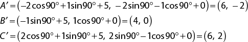
Recall the discussion of the unit circle from Chapter 4, “Vectors and Basic Physics.” The unit circle begins at the point (1, 0). A rotation of 90˚, or ![]() radians, is counterclockwise to the point (0, 1), a rotation of 180˚, or π radians, is the point (–1, 0), and so on. This is technically a rotation about the z-axis, even though you don’t draw the z-axis in a typical unit circle diagram.
radians, is counterclockwise to the point (0, 1), a rotation of 180˚, or π radians, is the point (–1, 0), and so on. This is technically a rotation about the z-axis, even though you don’t draw the z-axis in a typical unit circle diagram.
Using sine and cosine, you can rotate an arbitrary point (x, y) by the angle θ as follows:
![]()
Notice that both equations depend on the original x and y values. For example, rotating (5, 0) by 270˚ is as follows:
![]()
As with the unit circle, the angle θ represents a counterclockwise rotation.
Keep in mind that this is a rotation about the origin. Given a triangle centered around the object space origin, rotating each vertex would rotate the triangle about the origin.
Combining Transformations
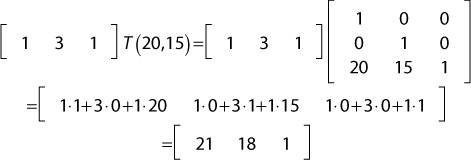
Although the preceding equations apply each transformation independently, it’s common to require multiple transformations on the same vertex. For example, you might want to both translate and rotate a quad. It’s important to combine these transformations in the correct order.
Suppose a triangle has the following points:

This original triangle points straight up, as in Figure 5.5(a). Now suppose you want to translate the triangle by (5, 0) and rotate it by 90˚. If you rotate first and translate second, you get this:
This results in the triangle rotated so that it points to the left and translated to the right, as in Figure 5.5(b).
If you reverse the order of the transformations so that you evaluate the translation first, you end up with this calculation:

In the case of translation first, rotation second, you end up with a triangle still facing to the left but positioned several units above the origin, as in Figure 5.5(c). This happens because you first move the triangle to the right, and then you rotate about the origin. Usually, this behavior is undesirable.

Because the order of transformations matter, it’s important to have a consistent order. For the transformation from object space to world space, always apply the transformations in the order scale, then rotation, then translation. Keeping this in mind, you could combine all three separate equations for scale, rotation, and translation into one set of equations to scale by (sx, sy), rotate by θ, and translate by (a, b):
![]()
Issues with Combining Equations
The combined equations derived in the previous section may seem like a solution to the problem: Take an arbitrary vertex in object space, apply the equations to each component, and you now have the vertex transformed into world space with an arbitrary scale, rotation, and position.
However, as alluded to earlier, this only transforms the vertices from object space to world space. Because world space is not normalized to device coordinates, you still have more transformations to apply in the vertex shader. These additional transformations typically do not have equations as simple as the equations covered thus far. This is especially because the basis vectors between these different coordinate spaces might be different. Combining these additional transformations into one equation would become unnecessarily complex.
The solution to these issues is to not use separate equations for each component. Instead, you use matrices to describe the different transformations, and you can easily combine these transformations with matrix multiplication.
Matrices and Transformations
A matrix is a grid of values, with 2×2 columns. For example, you could write a 2×2 matrix as follows, with a through d representing individual values in the matrix:

You use matrices to represent transformations in computer graphics. All the transformations from the preceding section have corresponding matrix representations. If you are experienced in linear algebra, you might recall that matrices can be used to solve systems of linear equations. Thus, it’s natural that you can represent the system of equations in the previous section as matrices.
This section explores some of the basic use cases of matrices in game programming. As with vectors, it’s most important to understand how and when to use these matrices in code. This book’s custom Math.h header file defines Matrix3 and Matrix4 classes, along with operators, member functions, and static functions that implement all the necessary features.
Matrix Multiplication
Much as with scalars, you can multiply two matrices together. Suppose you have the following matrices:

The result of the multiplication C = AB is:

In other words, the top-left element of C is the dot product of the first row of A with the first column of B.
Matrix multiplication does not require matrices to have identical dimensions, but the number of columns in the left matrix must be equal to the number of rows in the right matrix. For instance, the following multiplication is also valid:

Matrix multiplication is not commutative, though it is associative:
Transforming a Point by Using a Matrix
A key aspect of transformations is that you can represent an arbitrary point as a matrix. For example, you can represent the point p=(x, y) as a single row (called a row vector):
You can instead represent p as a single column (called a column vector):

Either representation works, but it’s important to consistently use one approach. This is because whether the point is a row or a column determines whether the point appears on the left- or right-hand side of the multiplication.
Suppose you have a transformation matrix T:

With matrix multiplication, you can transform the point p by this matrix, yielding the transformed point (x′,y′). However, whether p is a single row or a single column gives different results when multiplied by T.
If p is a row, the multiplication is as follows:

But if p is a column, the multiplication would yield the following:

This gives two different values for x′ and y′, but only one is the correct answer—because the definition of a transform matrix relies on whether you’re using row vectors or column vectors.
Whether to use row or column vectors is somewhat arbitrary. Most linear algebra textbooks use column vectors. However, in computer graphics there is a history of using either row or column vectors, depending on the resource and graphics API. This book uses row vectors, mainly because the transformations apply in a left-to-right order for a given point. For example, when using row vectors, the following equation transforms the point q by matrix T first and then by matrix R:
You can switch between row and column vectors by taking the transpose of each transform matrix. The transpose of the matrix rotates the matrix such that the first row of the original matrix becomes the first column of the result:

If you wanted to switch the equation to transform q using column vectors, you would calculate as follows:
The matrices in the remainder of this book assume that you are using row vectors. However, a simple transpose of these matrices converts them to work with column vectors.
Finally, the identity matrix is a special type of matrix represented by an uppercase l. An identity matrix always has an equal number of rows and columns. All values in the identity matrix are 0, except for the diagonal, which is all 1s. For example, the 3×3 identity matrix is as follows:

Any arbitrary matrix multiplied by the identity matrix does not change. In other words:
Transforming to World Space, Revisited
You can represent the scale, rotation, and translation transformations with matrices. To combine the transformations, instead of deriving a combined equation, multiply the matrices together. Once you have a combined world transform matrix, you can transform every vertex of the object by this world transform matrix.
As before, let’s focus on 2D transformations first.
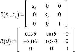
Scale Matrix
You can use a 2×2 scale matrix to apply the scale transformation:

For example, this would scale (1,3) by (5,2):

Rotation Matrix
A 2D rotation matrix represents a rotation (about the z-axis) by angle θ:

So, you can rotate (0,3) by 90˚ with the following:

Translation Matrices
You can represent 2D scale and rotation matrices with 2×2 matrices. However, there’s no way to write a generic 2D translation matrix of size 2×2. The only way to express the translation T(a,b) is with a 3×3 matrix:

However, you can’t multiply a 1×2 matrix representing a point by a 3×3 matrix because the 1×2 matrix doesn’t have enough columns. The only way you can multiply these together is if you add an additional column to the row vector, making it a 1×3 matrix. This requires adding an extra component to the point. Homogenous coordinates use n+1 components to represent an n-dimensional space. So, for a 2D space, homogeneous coordinates use three components.
Although it might seem reasonable to call this third component the z component, it’s a misnomer. That’s because you’re not representing a 3D space, and you want to reserve the z component for 3D spaces. Thus this special homogeneous coordinate is the w component. You use w for both 2D and 3D homogeneous coordinates. So, a 2D point represented in homogeneous coordinates is (x,y,w), while a 3D point represented in homogeneous coordinates is (x,y,z,w).
For now, you will only use a value of 1 for the w component. For example, you can represent the point p=(x,y) with the homogeneous coordinate (x,y,1). To understand how homogeneous coordinates work, suppose you wish to translate the point (1,3) by (20,15). First, you represent the point as a homogeneous coordinate with a w component of 1 and then you multiply the point by the translation matrix:
Note that, in this calculation, the w component remains 1. However, you’ve translated the x and y components by the desired amount.
Combining Transformations
As mentioned earlier, you can combine multiple transform matrices by multiplying them together. However, you can’t multiply a 2×2 matrix with a 3×3 matrix. Thus, you must represent the scale and rotation transforms with 3×3 matrices that work with homogeneous coordinates:
Now that you’ve represented the scale, rotation, and translation matrices as 3×3 matrices, you can multiply them together into one combined transform matrix. This combined matrix that transforms from object space to world space is the world transform matrix. To compute the world transform matrix, multiply the scale, rotation, and translation matrices in the following order:
This order of multiplication corresponds to the order in which you wish to apply the transformations (scale, then rotate, then translate). You can then pass this world transform matrix to the vertex shader and use it to transform every vertex of an object by its world transform matrix.
Adding World Transforms to Actor
Recall that the declaration of the Actor class already has a Vector2 for position, a float for scale, and a float for the angle rotation. You now must combine these different attributes into a world transform matrix.
First, add two member variables to Actor, a Matrix4 and a bool:
Matrix4 mWorldTransform;
bool mRecomputeWorldTransform;
The mWorldTransform variable obviously stores the world transform matrix. The reason you use a Matrix4 here instead of a Matrix3 is because the vertex layout assumes that all vertices have a z component (even though in 2D, you don’t actually need the z component). Since the homogenous coordinates for 3D are (x, y, z, w), you need a 4×4 matrix.
The Boolean tracks whether you need to recalculate the world transform matrix. The idea is that you want to recalculate the world transform only if the actor’s position, scale, or rotation changes. In each of the setter functions for the position, scale, and rotation of the actor, you set mRecomputeWorldTransform to true. This way, whenever you change these component properties, you’ll be sure to compute the world transform again.
You also initialize mRecomputeWorldTransform to true in the constructor, which guarantees to compute the world transform at least once for each actor.
Next, implement a CreateWorldTransform function, as follows:
void Actor::ComputeWorldTransform()
{
if (mRecomputeWorldTransform)
{
mRecomputeWorldTransform = false;
// Scale, then rotate, then translate
mWorldTransform = Matrix4::CreateScale(mScale);
mWorldTransform *= Matrix4::CreateRotationZ(mRotation);
mWorldTransform *= Matrix4::CreateTranslation(
Vector3(mPosition.x, mPosition.y, 0.0f));
}
Note that you use various Matrix4 static functions to create the component matrices. CreateScale creates a uniform scale matrix, CreateRotationZ creates a rotation matrix about the z-axis, and CreateTranslation creates a translation matrix.
You call ComputeWorldTransform in Actor::Update, both before you update any components and after you call UpdateActor (in case it changes in the interim):
void Actor::Update(float deltaTime)
{
if (mState == EActive)
{
ComputeWorldTransform();
UpdateComponents(deltaTime);
UpdateActor(deltaTime);
ComputeWorldTransform();
}
}
Next, add a call to ComputeWorldTransform in Game::Update to make sure any “pending” actors (actors created while updating other actors) have their world transform calculated in the same frame where they’re created:
// In Game::Update (move any pending actors to mActors)
for (auto pending : mPendingActors)
{
pending ->ComputeWorldTransform();
mActors.emplace_back(pending);
}
It would be nice to have a way to notify components when their owner’s world transform gets updated. This way, the component can respond as needed. To support this, first add a virtual function declaration to the base Component class:
virtual void OnUpdateWorldTransform() { }
Next, call OnUpdateWorldTransform on each of the actor’s components inside the ComputeWorldTransform function. Listing 5.10 shows the final version of ComputeWorldTransform.
Listing 5.10 Actor::ComputeWorldTransform Implementation
void Actor::ComputeWorldTransform()
{
if (mRecomputeWorldTransform)
{
mRecomputeWorldTransform = false;
// Scale, then rotate, then translate
mWorldTransform = Matrix4::CreateScale(mScale);
mWorldTransform *= Matrix4::CreateRotationZ(mRotation);
mWorldTransform *= Matrix4::CreateTranslation(
Vector3(mPosition.x, mPosition.y, 0.0f));
// Inform components world transform updated
for (auto comp : mComponents)
{
comp ->OnUpdateWorldTransform();
}
}
}
For now, you won’t implement OnUpdateWorldTransform for any components. However, you will use it for some components in subsequent chapters.
Although actors now have world transform matrices, you aren’t using the matrices in the vertex shader yet. Therefore, running the game with the code as discussed so far would just yield the same visual output as in Figure 5.3. Before you can use the world transform matrices in the shader, we need to discuss one other transformation.
Transforming from World Space to Clip Space
With the world transform matrix, you can transform vertices into world space. The next step is to transform the vertices into clip space, which is the expected output for the vertex shader. Clip space is a close relative of normalized device coordinates. The only difference is that clip space also has a w component. This was why you created a vec4 to save the vertex position in the gl_Position variable.
The view-projection matrix transforms from world space to clip space. As might be apparent from the name, the view-projection matrix has two component matrices: the view and the projection. The view accounts for how a virtual camera sees the game world, and the projection specifies how to convert from the virtual camera’s view to clip space. Chapter 6, “3D Graphics,” talks about both matrices in much greater detail. For now, because the game is 2D, you can use a simple view-projection matrix.
Recall that in normalized device coordinates, the bottom-left corner of the screen is (–1, –1) and the top-right corner of the screen is (1, 1). Now consider a 2D game that does not have scrolling. A simple way to think of the game world is in terms of the window’s resolution. For example, if the game window is 1024×768, why not make the game world that big, also?
In other words, consider a view of world space such that the center of the window is the world space origin, and there’s a 1:1 ratio between a pixel and a unit in world space. In this case, moving up by 1 unit in world space is the same as moving up by 1 pixel in the window. Assuming a 1024×768 resolution, this means that the bottom-left corner of the window corresponds to (–512, –384) in world space, and the top-right corner of the window corresponds to (512, 384), as in Figure 5.6.

Figure 5.6 The view of a world where the screen resolution is 1024×768 and there’s a 1:1 ratio between a pixel and a unit in world space
With this view of the world, it’s not too difficult to convert from world space into clip space. Simply divide the x-coordinate by width / 2 and divide the y-coordinate by height / 2. In matrix form, assuming 2D homogeneous coordinates, this simple view projection matrix is as follows:

For example, given the 1024×768 resolution and the point (256,192) in world space, if you multiply the point by SimpleViewProjection, you get this:

The reason this works is that you normalize the range [–512, 512] of the x-axis to [–1, 1], and the range of [–384, 384] on the y-axis [–1, 1], just as with normalized device coordinates!
Combining the SimpleViewProjection matrix with the world transform matrix, you can transform an arbitrary vertex v from its object space into clip space with this:
This is precisely what you will calculate in the vertex shader for every single vertex, at least until SimpleViewProjection has outlived its usefulness.
Updating Shaders to Use Transform Matrices
In this section, you’ll create a new vertex shader file called Transform.vert. It starts initially as a copy of the Basic.vert shader from Listing 5.3. As a reminder, you write this shader code in GLSL, not C++.
First, you declare two new global variables in Transform.vert with the type specifier uniform. A uniform is a global variable that typically stays the same between numerous invocations of the shader program. This contrasts in and out variables, which will change every time the shader runs (for example, once per vertex or pixel). To declare a uniform variable, use the keyword uniform, followed by the type, followed by the variable name.
In this case, you need two uniforms for the two different matrices. You can declare these uniforms as follows:
uniform mat4 uWorldTransform;
uniform mat4 uViewProj;
Here, the mat4 type corresponds to a 4×4 matrix, which is needed for a 3D space with homogeneous coordinates.
Then you change the code in the vertex shader’s main function. First, convert the 3D inPosition into homogeneous coordinates:
vec4 pos = vec4(inPosition, 1.0);
Remember that this position is in object space. So you next multiply it by the world transform matrix to transform it into world space, and then multiply it by the view-projection matrix to transform it into clip space:
gl_Position = pos * uWorldTransform * uViewProj;
These changes yield the final version of Transform.vert, shown in Listing 5.11.
Listing 5.11 Transform.vert Vertex Shader
#version 330
// Uniforms for world transform and view-proj
uniform mat4 uWorldTransform;
uniform mat4 uViewProj;
// Vertex attributes
in vec3 inPosition;
void main()
{
vec4 pos = vec4(inPosition, 1.0);
gl_Position = pos * uWorldTransform * uViewProj;
}
You then change the code in Game::LoadShaders to use the Transform.vert vertex shader instead of Basic.vert:
if (!mSpriteShader ->Load("Shaders/Transform.vert", "Shaders/Basic.frag"))
{
return false;
}
Now that you have uniforms in the vertex shader for the world transform and view-projection matrices, you need a way to set these uniforms from C++ code. OpenGL provides functions to set uniform variables in the active shader program. It makes sense to add wrappers for these functions to the Shader class. For now, you can add a function called SetMatrixUniform, shown in Listing 5.12, to Shader.
Listing 5.12 Shader::SetMatrixUniform Implementation
void Shader::SetMatrixUniform(const char* name, const Matrix4& matrix)
{
// Find the uniform by this name
GLuint loc = glGetUniformLocation(mShaderProgram, name);
// Send the matrix data to the uniform
glUniformMatrix4fv(
loc, // Uniform ID
1, // Number of matrices (only 1 in this case)
GL_TRUE, // Set to TRUE if using row vectors
matrix.GetAsFloatPtr() // Pointer to matrix data
);
}
Notice that SetMatrixUniform takes in a name as a string literal, as well as a matrix. The name corresponds to the variable name in the shader file. So, for uWorldTransform, the parameter would be "uWorldTransform". The second parameter is the matrix to send to the shader program for that uniform.
In the implementation of SetMatrixUniform, you get the location ID of the uniform with glGetUniformLocation. Technically, you don’t have to query the ID every single time you update the same uniform because the ID doesn’t change during execution. You could improve the performance of this code by caching the values of specific uniforms.
Next, the glUniformMatrix4fv function assigns a matrix to the uniform. The third parameter of this function must be set to GL_TRUE when using row vectors. The GetAsFloatPtr function is simply a helper function in Matrix4 that returns a float* pointer to the underlying matrix.
note
OpenGL has a newer approach to setting uniforms, called uniform buffer objects (abbreviated UBOs). With UBOs, you can group together multiple uniforms in the shader and send them all at once. For shader programs with many uniforms, this generally is more efficient than individually setting each uniform’s value.
With uniform buffer objects, you can split up uniforms into multiple groups. For example, you may have a group for uniforms that update once per frame and uniforms that update once per object. The view-projection won’t change more than once per frame, while every actor will have a different world transform matrix. This way, you can update all per-frame uniforms in just one function call at the start of the frame. Likewise, you can update all per-object uniforms separately for each object. To implement this, you must change how you declare uniforms in the shader and how you mirror that data in the C++ code.
However, at this writing, some hardware still has spotty support for UBOs. Specifically, the integrated graphics chips of some laptops don’t fully support uniform buffer objects. On other hardware, UBOs may even run more slowly than uniforms set the old way. Because of this, this book does not use uniform buffer objects. However, the concept of buffer objects is prevalent in other graphics APIs, such as DirectX 11 and higher.
Now that you have a way to set the vertex shader’s matrix uniforms, you need to set them. Because the simple view-projection won’t change throughout the course of the program, you only need to set it once. However, you need to set the world transform matrix once for each sprite component you draw because each sprite component draws with the world transform matrix of its owning actor.
In Game::LoadShaders, add the following two lines to create and set the view-projection matrix to the simple view projection, assuming a screen width of 1024×768:
Matrix4 viewProj = Matrix4::CreateSimpleViewProj(1024.f, 768.f);
mShader.SetMatrixUniform("uViewProj", viewProj);
The world transform matrix for SpriteComponent is a little more complex. The actor’s world transform matrix describes the position, scale, and orientation of the actor in the game world. However, for a sprite, you also want to scale the size of the rectangle based on the size of the texture. For example, if an actor has a scale of 1.0f, but the texture image corresponding to its sprite is 128×128, you need to scale up the unit square to 128×128. For now, assume that you have a way to load in the textures (as you did in SDL) and that the sprite component knows the dimensions of these textures via the mTexWidth and mTexHeight member variables.
Listing 5.13 shows the implementation of SpriteComponent::Draw (for now). First, create a scale matrix to scale by the width and height of the texture. You then multiply this by the owning actor’s world transform matrix to create the desired world transform matrix for the sprite. Next, call SetMatrixUniform to set the uWorldTransform in the vertex shader program. Finally, you draw the triangles as before, with glDrawElements.
Listing 5.13 Current Implementation of SpriteComponent::Draw
void SpriteComponent::Draw(Shader* shader)
{
// Scale the quad by the width/height of texture
Matrix4 scaleMat = Matrix4::CreateScale(
static_cast<float>(mTexWidth),
static_cast<float>(mTexHeight),
1.0f);
Matrix4 world = scaleMat * mOwner ->GetWorldTransform();
// Set world transform
shader ->SetMatrixUniform("uWorldTransform", world);
// Draw quad
glDrawElements(GL_TRIANGLES, 6, GL_UNSIGNED_INT, nullptr);
}
With the world transform and view-projection matrices added to the shader, you now can see the individual sprite components in the world at arbitrary positions, scales, and rotations, as in Figure 5.7. Of course, all the rectangles are just a solid color for now because Basic.frag just outputs blue. This is the last thing to fix to achieve feature parity with the SDL 2D rendering from the previous chapters.

Texture Mapping
Texture mapping is a technique for rendering a texture (image) on the face of a triangle. It allows you to use colors from a texture when drawing a triangle instead of using just a solid color.
To use texture mapping, you need an image file. Next, you need to decide how to apply textures to each triangle. If you have just the sprite rectangle, it makes sense that the top-left corner of the rectangle should correspond to the top-left corner of the texture. However, you can use texture mapping with arbitrary 3D objects in the game. For example, to correctly apply a texture to a character’s face, you need to know which parts of the texture should correspond to which triangles.
To support this, you need an additional vertex attribute for every vertex in the vertex buffer. Previously, the vertex attributes only stored a 3D position in each vertex. For texture mapping, each vertex also needs a texture coordinate that specifies the location in the texture that corresponds to that vertex.
Texture coordinates typically are normalized coordinates. In OpenGL, the coordinates are such that the bottom-left corner of the texture is (0, 0) and the top-right corner is (1, 1), as shown in Figure 5.8. The U component defines the right direction of the texture, and the V component defines the up direction of the texture. Thus, many use the term UV coordinates as a synonym for texture coordinates.

Because OpenGL specifies the bottom left of the texture as its origin, it also expects the image pixel data format as one row at a time, starting at the bottom row. However, a big issue with this is that most image file formats store their data starting at the top row. Not accounting for this discrepancy results in textures that appear upside down. There are multiple ways to solve this problem: invert the V-component, load the image upside down, or store the image on disk upside down. This book simply inverts the V component—that is, assumes that the top-left corner is (0, 0). This corresponds to the texture coordinate system that DirectX uses.
Each vertex of a triangle has its own separate UV coordinates. Once you know the UV coordinates for each vertex of a triangle, you can fill in every pixel in the triangle by blending (or interpolating) the texture coordinate, based on the distance from each of the three vertices. For example, a pixel exactly in the center of the triangle corresponds to a UV coordinate that’s the average of the three vertices’ UV coordinates, as in Figure 5.9.

Recall that a 2D image is just a grid of pixels with different colors. So, once you have a texture coordinate for a specific pixel, you need to convert this UV coordinate to correspond to a specific pixel in the texture. This “pixel in the texture” is a texture pixel, or texel. The graphics hardware uses a process called sampling to select a texel corresponding to a specific UV coordinate.
One complication of using normalized UV coordinates is that two slightly different UV coordinates may end up closest to the same texel in the image file. The idea of selecting the texel closest to a UV coordinate and using that for the color is called nearest-neighbor filtering.
However, nearest-neighbor filtering has some issues. Suppose you map a texture to a wall in a 3D world. As the player gets closer to the wall, the wall appears larger and larger onscreen. This looks like zooming in on an image file in a paint program, and the texture appears blocky or pixelated because each individual texel is very large onscreen.
To solve this pixelation, you can instead use bilinear filtering. With bilinear filtering, you select a color based on the blending of each texel neighboring the nearest neighbor. If you use bilinear filtering for the wall example, as the player gets closer, the wall seems to blur instead of appearing pixelated. Figure 5.10 shows a comparison between nearest-neighbor and bilinear filtering of part of the star texture.

We explore the idea of improving the quality of textures further in Chapter 13, “Intermediate Graphics.” For now, let’s enable bilinear filtering for all textures.
To use texture mapping in OpenGL, there are three things you need to do:
Load image files (textures) and create OpenGL texture objects.
Update the vertex format to include texture coordinates.
Update the shaders to use the textures.
Loading the Texture
Although you can use the SDL Image library to load images for OpenGL, the Simple OpenGL Image Library (SOIL) is a little easier to use. SOIL can read in several file formats, including PNG, BMP, JPG, TGA, and DDS. As it’s designed to work with OpenGL, it slots in easily with the other OpenGL code needed for creating a texture object.
Listing 5.14 gives the declaration of a Texture class that encapsulates loading in a texture file and using it with OpenGL. The names of the functions and member variables are mostly self-explanatory; for example, Load loads the texture from the file. For member variables, you have a width and height of the texture and an OpenGL texture ID.
Listing 5.14 Texture Declaration
class Texture
{
public:
Texture();
~Texture();
bool Load(const std::string& fileName);
void Unload();
void SetActive();
int GetWidth() const { return mWidth; }
int GetHeight() const { return mHeight; }
private:
// OpenGL ID of this texture
unsigned int mTextureID;
// Width/height of the texture
int mWidth;
int mHeight;
};
The implementation of Load contains the bulk of the Texture class code. You first declare a local variable to store the number of channels and then call SOIL_load_image to load in the texture:
int channels = 0;
unsigned char* image = SOIL_load_image(
fileName.c_str(), // Name of file
&mWidth, // Stores width
&mHeight, // Stores height
&channels, // Stores number of channels
SOIL_LOAD_AUTO // Type of image file, or auto for any
);
If SOIL fails to load the image file, SOIL_load_image returns nullptr. Therefore, you should add a check to make sure the image loaded.
Then you need to determine whether the image is RGB or RGBA. You can assume that this is based on the number of channels (three means RGB, four means RGBA):
int format = GL_RGB;
if (channels == 4)
{
format = GL_RGBA;
}
Next, use glGenTextures to create an OpenGL texture object (saving the ID in mTextureID) and glBindTexture to set the texture as active:
glGenTextures(1, &mTextureID);
glBindTexture(GL_TEXTURE_2D, mTextureID);
The GL_TEXTURE_2D target passed to glBindTexture is by far the most common texture target, but there are other choices for advanced types of textures.
Once you have an OpenGL texture object, the next step is to copy the raw image data into it with the glTexImage2D function, which takes quite a few parameters:
glTexImage2D(
GL_TEXTURE_2D, // Texture target
0, // Level of detail (for now, assume 0)
format, // Color format OpenGL should use
mWidth, // Width of texture
mHeight, // Height of texture
0, // Border – "this value must be 0"
format, // Color format of input data
GL_UNSIGNED_BYTE,// Bit depth of input data
// Unsigned byte specifies 8-bit channels
image // Pointer to image data
);
Once you’ve copied the image data to OpenGL, you can tell SOIL to free the image from memory:
SOIL_free_image_data(image);
Finally, use the glTexParameteri function to enable bilinear filtering:
glTexParameteri(GL_TEXTURE_2D, GL_TEXTURE_MIN_FILTER, GL_LINEAR);
glTexParameteri(GL_TEXTURE_2D, GL_TEXTURE_MAG_FILTER, GL_LINEAR);
For now, don’t worry about the parameters passed to glTexParameteri. (They are discussed further in Chapter 13, “Intermediate Graphics.”)
Listing 5.15 shows the final version of Texture::Load.
Listing 5.15 Texture::Load Implementation
bool Texture::Load(const std::string& fileName)
{
int channels = 0;
unsigned char* image = SOIL_load_image(fileName.c_str(),
&mWidth, &mHeight, &channels, SOIL_LOAD_AUTO);
if (image == nullptr)
{
SDL_Log("SOIL failed to load image %s: %s",
fileName.c_str(), SOIL_last_result());
return false;
}
int format = GL_RGB;
if (channels == 4)
{
format = GL_RGBA;
}
glGenTextures(1, &mTextureID);
glBindTexture(GL_TEXTURE_2D, mTextureID);
glTexImage2D(GL_TEXTURE_2D, 0, format, mWidth, mHeight, 0, format,
GL_UNSIGNED_BYTE, image);
SOIL_free_image_data(image);
// Enable bilinear filtering
glTexParameteri(GL_TEXTURE_2D, GL_TEXTURE_MIN_FILTER, GL_LINEAR);
glTexParameteri(GL_TEXTURE_2D, GL_TEXTURE_MAG_FILTER, GL_LINEAR);
return true;
}
The Texture::Unload and Texture::SetActive functions are each just a single line. Unload deletes the texture object, and SetActive calls glBindTexture:
void Texture::Unload()
{
glDeleteTextures(1, &mTextureID);
}
void Texture::SetActive()
{
glBindTexture(GL_TEXTURE_2D, mTextureID);
}
You can then load textures into a map in Game, much as you did for SDL_Texture previously. The Game::GetTexture function then returns a Texture* for the requested texture. Next, SpriteComponent needs a Texture* member variable instead of SDL_Texture*.
Finally, in SpriteComponent::Draw, add a call to SetActive on mTexture, right before drawing the vertices. This means you can now set a different active texture for each sprite component you draw:
// In SpriteComponent::Draw...
// Set current texture
mTexture ->SetActive();
// Draw quad
glDrawElements(GL_TRIANGLES, 6,
GL_UNSIGNED_INT, nullptr);
Updating the Vertex Format
To use texture mapping, the vertices need to have texture coordinates, so you need to update the sprite VertexArray:
float vertices[] = {
-0.5f, 0.5f, 0.f, 0.f, 0.f, // top left
0.5f, 0.5f, 0.f, 1.f, 0.f, // top right
0.5f, -0.5f, 0.f, 1.f, 1.f, // bottom right
-0.5f, -0.5f, 0.f, 0.f, 1.f // bottom left
};
Remember that the V texture coordinate is flipped to account for OpenGL’s idiosyncrasy with how it expects the image data.
For each vertex, the first three floating-point values are the position and the next two floating-point values are the texture coordinates. Figure 5.11 shows the memory layout of this new vertex format.

Because you’re changing the vertex layout, you must change code in the VertexArray constructor. For simplicity, assume that all vertices must have a 3D position and 2D texture coordinates. (You’ll change this in subsequent chapters.)
Because the size of each vertex has changed, you need to update the glBufferData call to specify that each vertex now has five floats per vertex:
glBufferData(GL_ARRAY_BUFFER, numVerts * 5 * sizeof(float),
verts, GL_STATIC_DRAW);
Because the index buffer is still the same, the glBufferData call for that doesn’t change. However, you must change vertex attribute 0 to specify that the stride of the vertex is now five floats:
glEnableVertexAttribArray(0);
glVertexAttribPointer(0, 3, GL_FLOAT, GL_FALSE,
sizeof(float) * 5, // The stride is now 5 floats
0); // Vertex position is still offset 0
This only fixes the position vertex attribute. However, because you now have a second vertex attribute for the texture coordinate, you must enable vertex attribute 1 and specify its format:
glEnableVertexAttribArray(1);
glVertexAttribPointer(
1, // Vertex attribute index
2, // Number of components (2 because UV)
GL_FLOAT, // Type of each component
GL_FALSE, // Not used for GL_FLOAT
sizeof(float) * 5, // Stride (usually size of each vertex)
reinterpret_cast<void*>(sizeof(float) * 3) // Offset pointer
);
The last parameter to this glVertexAttribPointer call is rather ugly. OpenGL needs to know the number of bytes from the start of a vertex to this attribute. That’s where the sizeof(float) * 3 comes from. However, OpenGL wants this as an offset pointer. Thus, you must use reinterpret_cast to coerce the type into a void* pointer.
tip
If you use a struct in C++ code to represent the format of the vertices, you can use the offsetof macro to determine the offsets to a vertex attribute rather than manually computing them. This is especially helpful if there is padding between vertex elements.
Updating the Shaders
Because the vertex format now uses texture coordinates, you should create two new shaders: Sprite.vert (initially a copy of Transform.vert) and Sprite.frag (initially a copy of Basic.frag).
The Sprite.vert Shader
There previously was only one vertex attribute, so you could just declare position as an in variable, and GLSL knew which vertex attribute it corresponded to. However, now that there are multiple vertex attributes, you must specify which attribute slot corresponds to which in variable. This changes the variable declarations to the following:
layout(location=0) in vec3 inPosition;
layout(location=1) in vec2 inTexCoord;
The layout directive specifies which attribute slot corresponds to which in variable. Here, you specify that there’s a 3D vector of floats for vertex attribute slot 0 and a 2D vector of floats for vertex attribute slot 1. This corresponds to the slot numbers in the glVertexAttribPointer calls.
Next, although the texture coordinates are an input to the vertex shader (because it’s in the vertex layout), the fragment shader also needs to know the texture coordinates. This is because the fragment shader needs to know the texture coordinates to determine the color at the pixel. Luckily, you can pass data from the vertex shader to the fragment shader by declaring a global out variable in the vertex shader:
out vec2 fragTexCoord;
Then, inside the vertex shader’s main function, add the following line, which copies the texture coordinates directly from the vertex input variable to the output variable:
fragTexCoord = inTexCoord;
The reason this ultimately works is that OpenGL automatically interpolates vertex shader outputs across the face of the triangle. Therefore, even though a triangle has only three vertices, any arbitrary pixel on the face of a triangle will know its corresponding texture coordinates in the fragment shader.
For completeness, Listing 5.16 gives the full source code for Sprite.vert.
Listing 5.16 Sprite.vert Implementation
#version 330
// Uniforms for world transform and view-proj
uniform mat4 uWorldTransform;
uniform mat4 uViewProj;
// Attribute 0 is position, 1 is tex coords.
layout(location = 0) in vec3 inPosition;
layout(location = 1) in vec2 inTexCoord;
// Add texture coordinate as output
out vec2 fragTexCoord;
void main()
{
// Convert position to homogeneous coordinates
vec4 pos = vec4(inPosition, 1.0);
// Transform position to world space, then clip space
gl_Position = pos * uWorldTransform * uViewProj;
// Pass along the texture coordinate to frag shader
fragTexCoord = inTexCoord;
}
The Sprite.frag Shader
As a rule, any out variables in the vertex shader should have a corresponding in in the fragment shader. The name and type of the in variable in the fragment shader must have the same name and type as the corresponding out variable in the vertex shader:
in vec4 fragTexCoord;
Next, you need to add a uniform for a texture sampler (that can get the color from a texture given a texture coordinate):
uniform sampler2D uTexture;
The sampler2D type is a special type that can sample 2D textures. Unlike with the world transform and view-projection uniforms in the vertex shader, you currently don’t need any code in C++ to bind this sampler uniform. This is because you currently bind only one texture at a time, so OpenGL automatically knows that the only texture sampler in the shader corresponds to the active texture.
Finally, replace the outColor assignment in the main function with the following:
outColor = texture(uTexture, fragTexCoord);
This samples the color from the texture, using the texture coordinates received from the vertex shader (after the coordinates interpolate across the face of the triangle).
Listing 5.17 shows the full source code for Sprite.frag.
Listing 5.17 Sprite.frag Implementation
#version 330
// Tex coord input from vertex shader
in vec2 fragTexCoord;
// Output color
out vec4 outColor;
// For texture sampling
uniform sampler2D uTexture;
void main()
{
// Sample color from texture
outColor = texture(uTexture, fragTexCoord);
}
You then change the code in Game:LoadShaders to now load Sprite.vert and Sprite.frag. The previous code inside the various actors that set textures on SpriteComponents now also successfully loads the textures with SOIL. With this code, you can now draw sprites with texture mapping, as shown in Figure 5.12. Unfortunately, there’s still one last issue to fix. Right now, the code is drawing black for pixels that should be transparent.

Alpha Blending
Alpha blending determines how to blend pixels with transparency (an alpha channel less than 1). Alpha blending uses an equation in the following form to calculate the pixel color:
In this equation, the source color is the color for the new source you’re drawing (from the fragment shader), and the destination color is the color that’s already in the color buffer. You can customize the alpha blending function by specifying the factor parameters.
To get the desired alpha blending result for transparency, you set the source factor to the alpha of the pixel you’re drawing (the source alpha) and the destination factor to one minus source alpha:
For example, suppose you have 8 bits per color, and the color buffer at some pixel is red. In this case, this is the destination color:
Next, say that you want to draw a pixel that’s blue; this is the source color:
Now suppose the source alpha is zero, meaning the pixel is completely transparent. In this case, our equation evaluates to the following:
This is the result you want for a fully transparent pixel. You completely ignore the source color if the alpha is zero and just use whatever color is already in the color buffer.
To enable this in code, add the following to Game::GenerateOuput, right before drawing all the sprites:
glEnable(GL_BLEND);
glBlendFunc(
GL_SRC_ALPHA, // srcFactor is srcAlpha
GL_ONE_MINUS_SRC_ALPHA // dstFactor is 1 - srcAlpha
);
The glEnable call says to turn on color buffer blending (which is disabled by default). Then you use glBlendFunc to specify the srcFactor and dstFactor that you want.
With alpha blending in place, the sprites now look correct, as shown in Figure 5.13. The 2D OpenGL rendering code now has feature parity with the previous use of SDL 2D rendering. It took a lot of work to get here, but the advantage is that the game code now has the foundations for 3D graphics support, which is the topic of Chapter 6.

Game Project
This chapter’s game project demonstrates all the code to convert the game code from SDL graphics to OpenGL. It converts the Asteroids game project from Chapter 3 to instead use OpenGL. The controls are the same as in Chapter 3: WASD to move the ship and spacebar to fire lasers. The code is available in the book’s GitHub repository, in the Chapter05 directory. Open Chapter05-windows.sln on Windows and Chapter05-mac.xcodeproj on Mac.
Summary
Because graphics hardware is optimized for polygons, 2D and 3D games internally use polygons (usually triangles) to represent all graphical objects in the world. Even a 2D sprite that you might think of as an image is a rectangle with a texture mapped to it. To send triangles to the graphics hardware, you must declare the attributes of each vertex and create a vertex and an index buffer.
All modern graphics APIs expect a programmer to use vertex and fragment (pixel) shaders to specify how polygons should render. You write these shaders as separate programs in a shader programming language (not C++). The vertex shader minimally outputs the vertex position in clip space, while the fragment shader determines the final color at a pixel.
Transformations allow you to draw several instances of the same object without needing separate vertex and index buffers for each instance. Object space is the coordinate space relative to the origin of an object, while world space is the coordinate space relative to the game world.
Games use matrices to represent transformations, and there are several different matrices for transformations, such as scale, rotation, and translation. Combining these transformations in the order scale, rotate, and translate yields a world transform matrix that can transform from object space to world space. To convert from world space to clip space, you use the view-projection matrix. For 2D games, you can simplify this by making 1 unit in world space equivalent to 1 pixel in the window.
Texture mapping applies part of a texture to the face of a triangle. To implement this, you need texture (UV) coordinates as a vertex attribute. In the fragment shader, you sample the texture color from the UV coordinate. This can either be based on the color of the texture pixel (texel) nearest to the UV coordinate, or it can be based on a bilinear filtering that considers nearby texels.
Finally, even though the task seems trivial, displaying sprites in OpenGL requires a lot of code. First, you must initialize OpenGL and GLEW. Next, to render any triangles, you must create a vertex array object, specify a vertex layout, write a vertex and pixel shader, and write code to load these shader programs. To transform the vertices from object space to clip space, you have to use uniforms to specify the world transform and view-projection matrices. To add texture mapping, you have to load an image, change the vertex layout to include UV coordinates, and update the shaders to sample from the texture.
Additional Reading
There are many excellent online references for aspiring OpenGL developers. The official OpenGL reference pages are useful for finding out what the parameters for each function do. Of all the OpenGL tutorial sites, one of the best is Learn OpenGL. For an extensive look at the graphical techniques used in game development, Real-Time Rendering by Thomas Akenine-Moller et al. is a definitive reference.
Akenine-Moller, Thomas, Eric Haines, and Naty Hoffman. Real-Time Rendering, 3rd edition. Natick: A K Peters, 2008.
Learn OpenGL. Accessed November 24, 2017. http://learnopengl.com/.
OpenGL Reference Pages. Accessed November 24, 2017. https://www.opengl.org/sdk/docs/man/.
Exercises
The exercises for this chapter involve making some modifications to this chapter’s game project to gain more experience using various OpenGL functions.
Exercise 5.1
Modify the background clear color so that it smoothly changes between colors. For example, starting from black, smoothly change over several seconds to blue. Then select another color (such as red) and smoothly change over several seconds to this other color. Think about how you can use deltaTime in Game::Update to facilitate this smooth transition.
Exercise 5.2
Modify the sprite vertices so that each vertex also has an RGB color associated with it. This is known as a vertex color. Update the vertex shader to take the vertex color as an input and pass it to the fragment shader. Then change the fragment shader so that rather than simply drawing the color sampled from the texture, it averages the color between the vertex color and texture color.