
All of the models that we worked on, until now, were 2D convolutions. This chapter will introduce the notion of using 3D convolutions.
There are a few basic ideas to understand how to use 3D convolutions:
- For one dimensional (1D) arrays, we're going to compute weights and then approximate a value for each of the arrays. This diagram represents the approximations graphically:
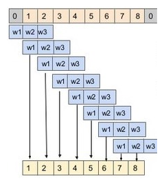
Figure: 1D convolution across a 1D array to understand features pertaining to this array
- We've been working with two dimensional arrays; for example images, are a 2D array of points. When computing the convolutions over an image, there are two important terms:
- Kernel – how many pixels you aggregate in the convolution computation
- Stride – how many pixels you move the kernel to compute the next kernel
The following diagram explains this step:

Figure: A 2D convolution example of taking a portion of a 2D image and producing a compressed representation
- Now, we have a 3D array of data and we'll use similar convolutional layers to traverse a kernel over the data. The following diagram illustrates this action:

Figure: A 3D convolution example of taking a portion of an 3D image and producing a compressed representation of that image
With 3D convolutions, you have stride and kernel in three dimensions. One of the pitfalls of 3D convolutions is that they haven't yet implemented sparse arrays – that is to say, that the convolutional layer has to traverse the entire array instead of only computing convolutions on occupied pixels.
Next, we are going to move on to preparing our environment to use this new technique!