CHAPTER 1

VALUATION ALGEBRAS

The valuation algebra framework provides the algebraic foundation for the application of all generic inference mechanisms introduced in this book and therefore marks the beginning of our studies. Comparable to the total order that is required for the application of sorting procedures, all formalisms must satisfy the structure of a valuation algebra in order to be processed by these generic inference tools. Further, this framework mirrors all the essential properties we naturally associate with the rather imprecise notions of knowledge and information. Let us engross ourselves in this thought and put our daily perception of information into words: information exists in pieces and comes from different sources. A piece of information refers to some specific questions that we later call the domain of an information piece. Also, there are two principal operations to manipulate information: we may combine or aggregate pieces of information to a new information piece and we may project a piece of information to some specific question which corresponds to information extraction. Depending on the operation, we either get a broader or more focused information. In the following section, we give a formal definition of the valuation algebra framework consisting of its operations and axioms. Along the way, we further bear on our idea of valuations as pieces of knowledge or information to clarify the rather abstract and formal structures.

1.1 OPERATIONS AND AXIOMS

The basic elements of a valuation algebra are so-called valuations that we subsequently denote by lower-case Greek letters , ψ, … Intuitively, a valuation can be regarded as a representation of information about the possible values of a finite set of variables. We use Roman capitals X, Y, … to refer to variables and lower-case letters s, t, … for sets of variables. Thus, we assume that each valuation refers to a finite set of variables d(), called its domain. For an arbitrary, finite set of variables s, Φs denotes the set of all valuations with d() = s. With this notation, the set of all possible valuations for a countable set of variables r can be defined as

Let D = P(r) be the powerset (the set of all subsets) of r and Φ the set of valuations with their domains in D. We assume the following operations defined in Φ, D:

These are the three basic operations of a valuation algebra. If we readopt our idea of valuations as pieces of information, the labeling operation tells us to which questions (variables) such a piece refers. Combination can be understood as aggregation of information and projection as the extraction of the part we are interested in. Sometimes this operation is also called focusing or marginalization. We now impose the following set of axioms on Φ and D:

(A1) Commutative Semigroup: Φ is associative and commutative under ⊗.

(A2) Labeling: For , ψ Φ,

(1.1)

(A3) Projection: For

(1.2)

(A4) Transitivity: For Φ and x ⊆ y ⊆ d(),

(1.3)

(A5) Combination: For , ψ Φ with d() = x, d(ψ) = y and z D such that x ⊆ z ⊆ x ∪ y,

(1.4)

(A6) Domain: For Φ with d() = x,

(1.5)

These axioms require natural properties regarding knowledge or information. The first axiom indicates that Φ is a commutative semigroup under combination. If information comes in pieces, the sequence of their aggregation does not influence the overall result. The labeling axiom tells us that the combination of valuations yields knowledge about the union of the involved domains. Variables do not vanish, nor do new ones appear. The projection axiom expresses the natural functioning of focusing. Transitivity says that projection can be performed in several steps. For the combination axiom, let us assume that we have some information about a domain in order to answer a certain question. Then, the combination axiom states how the answer is affected if a new information piece arrives. We can either combine the new piece to the given information and project afterwards to the specified domain, or first remove the uninteresting parts of the new information and combine it afterwards. Both approaches lead to the same result. In fact, we are going to see in Section 5.3 that this axiom correlates with some generalized distributive law. Finally, the domain axiom ensures that information is not influenced by projection to its own domain, which expresses some kind of stability with respect to trivial projection.

Definition 1.1 A system Φ, D together with the operations of labeling, projection and combination satisfying these axioms is called a valuation algebra.

In the first appearance of the valuation algebra axioms (Shafer & Shenoy, 1988; Shenoy & Shafer, 1990) only Axioms (A1), (A4) and a simpler version of (A5) were listed. Axiom (A2) was simply assumed in the definition of combination. (Shafer, 1991) mentioned Property (A3) for the first time and also remarked that Axiom (A6) cannot be derived from the others. (Kohlas, 2003) then assembled these early results to a complete and sufficient axiomatic system for generic inference and local computation. But in addition to the above system, all former approaches contained so-called neutral valuations that express vacuous information with respect to a certain domain. Here, we will introduce valuation algebras with neutral elements in Section 3.3 as a special case of the definition given here.

Before we turn towards the first concrete examples of valuation algebras, we list a few elementary properties that are derived directly from the above set of axioms.

Lemma 1.1

Proof:

1.2 FIRST EXAMPLES

Our first encounter with the valuation algebra framework took place on a very abstract level. To reward the reader for this formal effort, we now consider a first catalogue of concrete formalisms that satisfy the valuation algebra structure. Such formalisms are subsequently called valuation algebra instances. For the moment, we content ourselves with the observation of how these formalisms fit in the valuation algebra framework. Later sections then inform about their exact purpose and semantics. However, these instances are all based on the important concepts of configurations, tuples or vectors that shall first be introduced separately.

Frames, Tuples, Configurations and Vectors:

Consider a countable set r of variables where each variable Xi r is referenced by its index i . Conversely, every index i refers to a unique variable Xi r. This one-to-one correspondence between variables and indexes allows us subsequently to identify the two concepts. Further, we assume for every variable X r a set ΩX of possible values, called its frame. Such variable frames are sometimes assumed to be finite or countable, but this is not a general requirement. If a frame contains exactly two elements, the corresponding variable is said to be binary. Moreover, if the two elements represent the states true and false, the variable is called propositional or Boolean. A tuple or configuration with finite domain s ⊆ r is a function

that associates a value x(X) ΩX with each variable X s. By convention, the single tuple with empty domain is identified by the diamond symbol , and we use bold-face, lower-case letters x, y, … to refer to tuples. Subsequently, we write x Ωs to mark x as a tuple with domain s, for which we also use the shorthand term s-tuple or s-configuration.

It is often convenient to decompose tuples according to some variable partition. This operation is also called projection, although it is not directly related to valuation algebras. Given an s-tuple x and t ⊆ s, the projection of x to t is defined by a t-tuple y such that y (X) = x(X) for all X t. We subsequently write x↓t for the projection of x to t. Note that denotes the projection of any tuple to the empty set. Further, this notation allows us to write x = (x↓t, x↓s-t) for the decomposition of x with respect to t and s − t. Observe also that (x, ) = (, x) = x. Similar to frames of single variables, the set Ωs represents all possible s-tuples and is therefore called the frame of the variable or index set s. In particular, Ωø = {}. Then, a tuple set with domain s is simply a subset S ⊆ Ωs. If a tuple set consists of only one element, then it is also called a singleton.

Example 1.1 To describe the attributes color, speed and prize of a car, we assume the set of variables r = {C, S, P} with variable frames: ΩC = {red, blue, black}, ΩS = {slow, fast} and ΩP = . Two possible r-tuples are x = (blue, fast, 30‘000) and y = (black, slow, 10‘000). The tuple x can for example be decomposed into x↓{C, P} = (blue, 30‘000) and x↓{S} = (fast). Further, the variable set {C, S} possesses the frame Ω{C, S} = {(red, slow), (blue, slow), …, (black, fast)}. Observe also that the frame Ωr contains infinitely many tuples.

If X r is a variable that takes real numbers, we have ΩX = , and for a set s ⊆ r of real variables the linear space s corresponds to the frame of all s-tuples. In this case, s-tuples are also called s-vectors. It is possible to introduce an extension operator that lifts an s-vector x to some larger domain t ⊆ s by assigning zeros to all variables in t − s. We thus have x↑t(X) = x(X) if X s and x↑t(X) = 0 otherwise. Clearly, the introduction of this operation is not only possible for real number but for all algebraic structures that contain a zero element. These definitions of frames, tuples and tuple sets allow for a uniform notation in the following tour through a first collection of valuation algebra instances.

1.1 Indicator Functions - Boolean Functions - Crisp Constraints

An indicator function with domain s ⊆ r identifies a subset S ⊆ Ωs by specifying for each tuple x Ωs whether x belongs to S or not. If we adopt the usual interpretation of 0 for x not being an element of S and 1 for x being in S, an indicator function i is defined by

Thus, an indicator i with domain d(i) = s is a function that maps every tuple x Ωs onto a value i(x) {0, 1}, i.e. i: Ωs → {0, 1}. These are the valuations in the valuation algebra of indicator functions. As introduced in Section 1.1, we usually write Φs for the set of all indicator functions with domain s and Φ for the set of all possible indicator functions over subsets of r. Combination of indicator functions is defined by multiplication. If i1 and i2 are indicator functions with domain s and t respectively, we define for x Ωs∪t

Alternatively, we may also define combination in terms of minimization:

Projection, on the other hand, corresponds to maximization. For an indicator i with domain s and t ⊆ s we define for all x Ωt

If we consider only variables with finite frames, an indicator function with domain s can be represented by an |s|-dimensional table with |Ωs| zero-one entries. Below, we simply use a relational or tabular representation, but emphasize that indicator functions are not limited to this inefficient representation. In order to prove that indicator functions form a valuation algebra, the reader may verify that all axioms are satisfied. However, in Section 5.3 this proof will be made for a whole family of formalisms that also includes indicator functions. Otherwise, a direct proof can be found in (Kohlas, 2003). Depending on its application field, the formalism of indicator functions has different names. In the context of constraint reasoning, they are usually called crisp constraints. Otherwise, indicator functions for propositional variables are also called Boolean functions.

For a concrete example of computing with indicator functions, consider a set of variables r = {A, B, C} with frames ΩA = {a, }, ΩB = {b, } and ΩC = {c, }. Then, assume two indicator functions i1 and i2 with domains d(i1) = {A, B} and d(i2) = {B, C}:

We combine i1 and i2 and project the result to {A}:

1.2 Relational Algebra

The second instance we are going to study is closely related to the first one. It is a subset of the relational algebra (Maier, 1983; Ullman, 1988), which traditionally belongs to the most fundamental formalisms for representing knowledge and information. In its usual extent, at least six operations are provided to manipulate knowledge represented as sets of tuples. Respecting the language of relational database theory, variables are called attributes and sets of tuples are called relations. A relation over s ⊆ r is therefore simply a tuple set R ⊆ Ωs. It is important to note that variable frames do not need to be finite and consequently, relations can also be infinite sets. Combination is defined by natural join: If R1 and R2 are relations with domain s and t respectively, we define

(1.8)

Projection is defined for a relation R with domain s and t ⊆ s as

Alternatively, the notation πt(R) = R↓t is also used in the context of relational algebras. If we consider only finite variables in r, then the relational algebra over r is isomorphic to the valuation algebra of indicator functions over r. In fact, relations are just another representation of indicators. We obtain the relation R associated to the indicator function with domain d() = s by

(1.9)

Conversely, we derive the indicator function associated to a relation R with domain s ⊆ r by (x) = 1 if x R, and (x) = 0 otherwise, for all x Ωs. Hence, we directly conclude that relations form a valuation algebra in the case of finite variables. This statement also holds for the general case as is will be shown in Chapter 7.3. Let us write the combination axiom for z = x in the notation of relational algebra: For R1, R2 Φ with d(R1) = x and d(R2) = y,

The right-hand side is called semi-join in database theory (Maier, 1983).

To give an example of computing in the relational algebra, we consider two relations R1 and R2 with domain d(R1) = {continent, country} and d(R2) = {country, city}:

Combining R1 and R2 gives

and we obtain for the projection of R3 to {continent}:

1.3 Arithmetic Potentials - Probability Potentials

Probability potentials are perhaps the most cited example of a valuation algebra, and their common algebraic structure with belief functions was originally the guiding theme for the abstraction process that lead to the valuation algebra framework (Shafer & Shenoy, 1988). However, at this point we yet ignore their usual interpretation as discrete probability mass functions and refer to this formalisms as arithmetic potentials. These are simple mappings that associate a non-negative real value with each tuple, i.e. p: Ωs → ≥0. Also, we consider from the outset only variables with finite frames and identify d(p) = s ⊆ r to be the domain of the potential p. The tabular representation can again be used for arithmetic potentials. Combination of two potentials p1 and p2 with domain s and t is defined by

(1.10)

for x Ωs∪t. Projection consists in summing up all variables to be eliminated. If arithmetic potentials are used to express discrete probability mass functions, then this corresponds to the operation of marginalization in probability theory. For a potential p with domain s,t ⊆ s and x Ωt, we define

(1.11)

Arithmetic potentials belong to the same family of instances as indicator functions. Section 5.3 provides a generic proof that all formalisms of this family satisfy the valuation algebra axioms. Moreover, we will also conclude from this result that other sets (such as integers, rational or complex numbers) may be used instead of real numbers to define arithmetic potentials.

We pointed out in the introduction of this book that the distributive law from arithmetics is used to make the computational process of inference more efficient. Also, we said that this property is contained in the valuation algebra axioms. This becomes evident by writing the combination axiom in the notation of arithmetic potentials: For p1, p2 Φ with d(p1) = s, d(p2) = t and x Ωs

For an example of how to compute with arithmetic potentials, consider a set r = {A, B, C} of three variables with finite frames ΩA = {a, }, ΩB = {b, } and ΩC = {c, }. We define two arithmetic potentials p1 and p2 with domain d(p1) = {A, B} and d(p2) = {B, C}:

We combine p1 and p2 and project the result to {A, C}:

1.4 Set Potentials - Belief Functions

As we already mentioned, belief functions (Shafer, 1976; Kohlas & Monney, 1995) rank among the few instances that originally initiated the abstraction process culminating in the valuation algebra framework (Shafer & Shenoy, 1988). Belief functions are special cases of set potentials. Therefore, we first focus on this slightly more general formalism and refer to Instance D.9 and D.6 for a discussion of belief functions and its alternative representations. The theory is again restricted to variables with finite frames. A set potential m: P(Ωs) → ≥0 with domain d(m) = s ⊆ r is a function that assigns non-negative real numbers to all subsets of the variable set frame Ωs. Combination of two set potentials m1 and m2 with domains s and t is defined for all tuple sets A ⊆ Ωs∪t by

(1.12)

This is a simplified version of Dempster’s rule of combination (Dempster, 1968; Shafer, 1991). Projection of a set potential m with domain s to t ⊆ s is given for A ⊆ Ωt by

(1.13)

Observe that these definitions use the language from the relational algebra to deal with tuple sets. This particular notation will later be helpful. Since relations satisfy the valuation algebra axioms, we may call in its properties to derive important results about set potentials. Note also that the formalism of set potentials essentially differs from the other instances introduced beforehand that map single tuples to some value. Indeed, it belongs to a second family of valuation algebras that will be introduced in Section 5.7 where we also provide a generic proof that all formalisms of this family satisfy the valuation algebra axioms. Before presenting a concrete example, it is important to remark that although all variable frames are finite, a simple enumeration of all assignments as proposed for indicator functions or arithmetic potentials is beyond question since set potentials assign values to all elements of the powerset of Ωs. Instead, only those entries are listed whose values differ from zero. These tuple sets are usually called focal sets.

Consider a set of two variables r = {A, B} with finite frames ΩA = {a, } and ΩB = {b, }. We define two set potentials m1 and m2 with domains d(m1) = {A, B} and d(m2) = {A}:

The task of computing the combination of m1 and m2 is simplified by constructing the following table as an intermediate step. The first column contains m1 and the top row m2, both extended to the union domain d(m1) ∪ d(m2) = {A, B}. Then, every internal cell contains the intersection between the two corresponding tuple sets and the product of the corresponding values. This corresponds to the natural join in equation (1.12).

To complete the combination, it is then sufficient to add the values of all internal cells with equal tuple set. The result of the combination is projected afterwards to {A} using equation (1.13)

1.5 Density Functions

All instances discussed so far are based on variables with finite (or at least countable) frames. Although such a setting is typical for a large number of formalisms used in computer science, it is in no way mandatory. Thus, we next introduce the valuation algebra of density functions which are defined over variables taking values from the set of real numbers. For a set of variables s ⊆ r, a density function f: s → ≥0 with domain s is a continuous, non-negative valued function with finite Riemann integral,

(1.14)

Note that x denotes a vector in the linear space Ωs = s. The combination f ⊗ g of two density functions f and g with domain s and t is defined for x s∪t by simple multiplication

(1.15)

The projection f↓t of a density f with d(f) = s to t ⊆ s is given by the integral

(1.16)

where x ⊆ t and y s-t. Density functions together with the above definitions of combination and projection form a valuation algebra. The proof of this statement even for the more general case of Lebesque measurable density functions can be found in (Kohlas, 2003). The perhaps most interesting example of a density function in the context of valuation algebras is the Gaussian density. In fact, Instance 1.6 below shows that Gaussian densities are closed under combination and projection and therefore establish a subalgebra of the valuation algebra of density functions.

Labeled Matrices

These first examples were all based on tuples and tuple sets. Next, we are going to introduce two further valuation algebra instances based on labeled matrices. For finite sets s,t ⊆ r a labeled, real-valued matrix is a mapping M: s × t → such that for X s and Y t we have M(X, Y) . We write M(, s × t) for the set of matrices of this kind. The sum of M1, M2 M(, s × t) is defined by

(1.17)

for X s and Y t. If M1 M(, s × t) and M2 M(, t × u) for s,t,u ⊆ r, X s and Y u we define the product M1 ˙ M2 by

(1.18)

A special element of the set M(, s × t) is the zero matrix defined for X s and Y t by O(X, Y) = 0. The projection of a labeled matrix M M(, s × t) to u ⊆ s and v ⊆ t is defined by M↓u,v (X, Y) = M(X, Y) if X u and Y v, which simply corresponds to dropping the unrequested rows and columns. Similarly to the extension of vectors, we extend a labeled matrices M M(, s × t) to u ⊇ s and v ⊇ t with X u and Y v by

(1.19)

Of special interest are often square matrices M M(, s × s). We then say that the domain of M is d(M) = s and use the abbreviation M (, s) for the set of all matrices with domain s. Also, the projection of a matrix M with domain s to t ⊆ s is abbreviated by M↓s and accordingly, we write M↑u for its extension to the larger domain u ⊆ s. Finally, we define the identity matrix for the domain s by I(X, Y) = 1 if X = Y and I(X, Y) = 0 otherwise. In later chapters, we will also consider labeled matrices with values from other algebraic structures than real numbers. But for the introduction of the following instances, the limitation to real numbers is sufficient.

1.6 Gaussian Densities - Gaussian Potentials

An important family of density functions is provided by Gaussian distributions. For a set of real variables s ⊆ r and x s a Gaussian density is defined by

(1.20)

where μ s denotes the mean vector and K: s × s → the symmetric and positive definite concentration matrix. The matrix K−1 is the variance-covariance matrix of the Gaussian density. Looking at this definition, we remark that a Gaussian density is completely determined by its mean vector and concentration matrix. Such pairs (μ, K) with μ s and K M(, s) being symmetric and positive definite are called Gaussian potentials. The square root in front of the exponential function in equation (1.20) is merely a normalization factor guaranteeing that the integral over the density function equals one.

Let f and g be two Gaussian densities with domain d(f) = s and d(g) = t, represented by the Gaussian potentials (μ1, K1) and (μ2, K2). When combining these two densities by equation (1.15) we can neglect the normalization constants and simply multiply the exponential functions. This in turn means adding their exponents. Doing so, we may also neglect additive terms without variables, since these terms simply go into the normalization factor. In the following, equality must always be taken up to such terms. We then get for the exponent of the combined density function and x s∪t

Define now

Note that K is still symmetric and positive definite. Then, we rewrite the last expression using K, add a constant, additive term to the last expression completing it to a quadratic form:

This finally means that the multiplication of two Gaussian densities results again in a Gaussian density with concentration matrix

(1.21)

and mean vector

(1.22)

Motivated by this result, we may define the combination of two Gaussian potentials (μ1, K1) and (μ2, K2) with d(μ1, K1) = s and d(μ2, K2) = t by

where μ is defined by (1.22) and K by (1.21). We found this combination rule by a purely formal derivation. Its reason and meaning will be given in Section 10.1. The projection of a Gaussian density f with domain d(f) = s, mean vector μ and concentration matrix K to a subset t ⊆ s is again a Gaussian density, as it will be shown in Appendix J.2. Its mean vector is simply μ−t and ((K−1)↓t)−1 is its concentration matrix. Consequently, Gaussian densities are closed under combination and projection and form an important subalgebra of the valuation algebra of density functions. The operations of combination and projection can both be expressed in terms of the Gaussian potentials associated with the densities. Gaussian densities and Gaussian potentials will be studied in detail in Chapter 10, which will also clarify the interest in this valuation algebra.

Many further valuation algebra instances will be introduced throughout the subsequent chapters. At this point we interrupt the study of formalisms for the time being and focus on the computational interest in valuation algebras. The following chapter phrases an abstract computational task called inference problem using the language of valuation algebras and also gives a first impression of the different semantics of this problem under different valuation algebra instances. But first, we propose a more far-reaching discussion of the valuation algebra axiomatics in the appendix of this chapter. The valuation algebra framework presented in Section 1.1 is more general than most of its antecessors. Nevertheless, there is still potential for further generalizations. Two such systems will be presented in the following appendix: the first introduces valuation algebras that are no more necessarily based on variable systems. Instead, valuations take their domains from a more general lattice structure. The second framework focuses on a generalization of the projection operator. Here, it is no longer the case that projections on arbitrary subsets are possible, but there is a fourth operator that tells us to which domain a valuation is allowed to be projected. For the understanding of the subsequent chapters, these systems are of minor importance. But it is nevertheless interesting to see that further instances can be covered by a more general and abstract definition of the valuation algebra framework, which still provides enough structure for the application of local computation.

1.3 CONCLUSION

This first chapter introduced the valuation algebra framework upon which all following chapters are based. Valuations can be imagined as pieces of information that refer to a question called the domain of the valuation. This domain is returned by the labeling operation. Two further operations called combination and projection are used to manipulate valuations. Combination corresponds to aggregation, and projection to focussing or extraction of knowledge. In addition, the valuation algebra framework consists of a set of six axioms that determine the behaviour of the three operations. Formalisms that satisfy the structure of a valuation algebra are called instances and occur numerously in very different fields of mathematics and computer science. This chapter gave a first selection of instances including crisp constraints, arithmetic and probability potentials, Dempster-Shafer belief functions, density functions and the important family of Gaussian distributions.

Appendix: Generalizations of the Valuation Algebra Framework

We first give a formal definition of lattices with their main variations and refer to (Davey & Priestley, 1990) for an extensive discussion of these an related concepts.

A.1 ORDERED SETS AND LATTICES

Definition A.2 A preorder is a binary relation ≤ over a set P which is reflexive and transitive. We have for a,b,c P:

• a ≤ a (reflexivity);
• a ≤ b and b ≤ c implies that a ≤ c (transitivity).

A preorder is called partial order if it is antisymmetric, i.e. if

• a ≤ b and b ≤ a implies that a = b (antisymmetry).

A set with a partial order is also called a partially ordered set or simply an ordered set. Chapter 5 starts with an introduction to semiring theory that naturally offers a large number of examples for preorders and partial orders. We therefore refer to the numerous examples of semirings in Chapter 5 for concrete sets providing preorders and partial orders.

Definition A.3 Let P be an ordered set.

• P has a bottom element if there exists an element ⊥ P such that ⊥ ≤ x for all x P.
• P has a top element if there exists an element ⊥ P such that x ≤ ⊥ for all x P.

Definition A.4 Let P be a ordered set and S ⊆ P. An element u P is called supremum, least upper bound or join of S if

• x ≤ u for all x S;
• for any v P such that x ≤ v for all x S it holds that u ≤ v.

Likewise, an element u P is called infimum, greatest lower bound or meet of S if

• u ≤ x for all x S;
• for any v P such that v ≤ x for all x S it holds that v ≤ u.

If join or meet of a subset S ⊆ P exist, then they are always unique, and we write S for join and S for meet. Moreover, if S = {x, y} consists of two elements, we generally write x ∨ y or sup{x, y} for join and x ∧ y or inf {x, y} for meet.

Definition A.5 Let P be a non-empty, ordered set.

• If x ∨ y and x ∧ y exist for all x, y P, then P is called a lattice.
• If S and S exist for all subsets S ⊆ P, then P is called a complete lattice.

Lattices may satisfy further identities:

Definition A.6 Let L be a lattice.

• L is said to be bounded, if it has a bottom and a top element.
• L is said to be distributive, if for all a, b, c L

This definition lists both statements of distributivity, although they are in fact equivalent. The proof is given in (Davey & Priestley, 1990). Note also that every complete lattice is bounded.

Example A.2 (Powerset or Subset Lattice) For any set A we consider the set of all subsets called its powerset or subset lattice P(A). This set is partially ordered via set inclusion and forms a lattice with set intersection as meet a ∧ b = a b and set union as join a ∨ b = a ∪ b. The powerset lattice is distributive, complete and bounded by A itself and the empty set .

Example A.3 (Division Lattice) The set of ∪ {0} also forms a distributive lattice with the least common multiple as join lcm(a, b) = a ∨ b and the greatest common divisor as meet gcd(a, b) = a ∧ b. The order is defined by divisibility, i.e. a ≤ b if a divides b. This lattice is also bounded with 1 as bottom and 0 as top element.

An important source of non-distributive lattices are partitions:

A.1.1 Partitions and Partition Lattices

Partition lattices take a universal position among all lattices. (Grätzer, 1978) shows that every lattice is isomorph to some partition lattice.

Definition A.7 A partition π = {Bi: 1 ≤ i ≤ n} of a set U called universe consists of a collection of subsets Bi ⊆ U called blocks such that

• Bi ≠ Ø;
• Bi Bj = Ø for i ≠ j and 1 ≤ i.j ≤ n;
• 

Let Part(U) denote the set of all possible partitions of a universe U. It is then possible to introduce a partial order between its elements. For π1, π2 Part(U) we write π1 ≤ π2 if every block of π1 is contained in some block of π2. This is the case if, and only if, every block of π2 is a union of blocks from π1. We then also say that the partition π1 is finer than π2, or conversely that π2 is coarser than π1. The blocks of the infimum or meet of an arbitrary collection of partitions P ⊆ Part(U) corresponds to the non-empty intersections of all blocks contained in the partitions of P. The definition of the supremum or join especially for the case of universes with an infinite number of elements is more involved. We refer to (Grätzer, 1978) for a discussion of this aspect. Here, we directly conclude that the set Part(U) of all partitions of the universe U forms a complete lattice. The partition {{u}: u U} consisting of all one-element subsets of U is the lower bound, and the partition {U} is the upper bound. A lattice whose elements are partitions of a universe U is called partition lattice. They are sublattices of Part(U) and generally not distributive. The above refinement relation is the natural way of introducing an order relation between partitions. However, in the context of algebraic information theory (Kohlas, 2003) it is often useful to consider the inverse of the natural order, i.e. π2 ≤c π1 if, and only if, π1 ≤ π2 or equivalently, if π2 is coarser than π1. The motivation is that a finer partition expresses more information than a coarser partition.

Example A.4 (Interval Partitions) Let U = [a, b) be a semi-closed interval of real numbers. A sequence x0 < x1 < … < xn with x0 = a and xn = b establishes a partition π = {[xi,xi+i): 0 ≤ i ≤ n − 1}. If an interval partition π1 contains all elements of the sequence defining the partition π2, then every bloc of π1 is contained in some bloc of π2. In other words, π1 is a refinement of π2. The meet of two interval partitions is obtained from the union sequence, and the join from the intersection. If for example U = [0, 1) the partition for 0 < 0.2 < 0.4 < 0.6 < 0.8 < 1 is a refinement of the partition for 0 < 0.4 < 0.8 < 1. If furthermore π1 is given by the sequence 0 < 0.5 < 0.8 < 1 and π2 by 0 < 0.2 < 0.8 < 1, their meet is obtained from the sequence 0 < 0.2 < 0.5 < 0.8 < 1 and their join from 0 < 0.8 < 1.

A.2 VALUATION ALGEBRAS ON GENERAL LATTICES

The definition of a valuation algebra given at the beginning of this chapter is based on a particular lattice, namely on the powerset lattice of variables (see Example A.2). This lattice is distributive. However, it turns out that the valuation algebra framework can even be generalized to arbitrary lattices (Shafer, 1991; Kohlas, 2003). Thus, let D be a lattice with a partial order ≤ and the two operations meet ∧ and join ∨. We denote by Φ the set of valuations with domains in D and suppose the following three operations defined on Φ and D.

We impose the following set of axioms on Φ and D:

(A1’) Commutative Semigroup: Φ is associative and commutative under ⊗.

(A2’) Labeling: For , ψ Φ,

(A.1)

(A3’) Projection: For Φ, x D and x ≤ d(),

(A.2)

(A4’) Transitivity: For Φ and x ≤ y ≤ d(),

(A.3)

(A5’) Combination: For , ψ Φ with d() = x, d(ψ) = y and z D such that x ≤ z ≤ x ∨ y,

(A.4)

(A6’) Domain: For Φ with d() = x,

(A.5)

Clearly, this definition of a valuation algebra is more general than the framework introduced beforehand. It is indeed surprising that no further properties of the lattice are required to enable the application of local computation (Kohlas & Monney, 1995). We must, however, accept that not all properties of the more restricted concept of a valuation algebra are maintained. Although the subsequent chapters of this book are entirely based on variable systems, we nevertheless present an example from diagnostics that is based on a valuation algebra with domains from a more general lattice, i.e. from a lattice of partitions (Kohlas & Monney, 1995; Shafer et al., 1987).

Example A.5 Suppose that your car does not start anymore and you want to determine the cause of its failure. The tree of diagnoses shown in Figure A.1 provides a structural approach for the identification of the cause of failure. At the beginning, the list of possible diagnoses is fairly coarse and only contains the failure possibilities Ω1 = {a, b, c, d}. Note, however, that these options are mutually exclusive and collectively exhaustive. More precise statements are obtained by partitioning coarse diagnoses. Doing so, we replace diagnosis a by {e, f} and diagnosis c by {l, g, h} which leads to the new set of failure possibilities Ω2 = {e, f, b, l, g, h, d}. After a third specialization step we finally obtain Ω3 = {e, f, b, i, j, k, g, h, d}. These step-wise refined sets of diagnoses are called frames of discernment. When a frame Ωi is replaced by a finer frame Ωi+1 the substitution of a diagnosis by a set of more precise diagnoses is described by a mapping

(A.6)

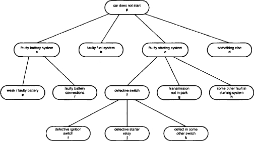
called refinement mapping or simply refinement (Shafer, 1976). Refinement mappings must satisfy the following requirements:

For example, the passage from Ω1 to Ω2 is expressed by the mapping

From an alternative but equivalent point of view, this family of related frames can be seen as a collection of partitions of the universe Ω3. These partitions are:

• π0 = {{e, f, b, i, j, k, g, h, d}};
• π1 = {{e, f}, {b}, {i, j, k, g, h}, {d}};
• π2 = {{e}, {f}, {b}, {i, j, k}, {g}, {h}, {d}};
• π3 = {{e}, {f}, {b}, {i}, {j}, {k}, {g}, {h}, {d}}.

Note that πi+1 ≤ πi, i.e. every block of πi+1 is contained in some block of πi. Because each frame Ωi corresponds to a partition πi, we may replace the frames in equation (A.6) by their corresponding partitions. The mapping

assigns to each block B πi the set of blocks in πi+1 whose union is B. The passage from π1 to π2 is thus expressed by the mapping

This mapping is referred to as decomposition mapping.

Although many valuation algebras with domains from variable lattices could be adapted to partition and other lattices, the modified valuation algebra of set potentials from Dempster-Shafer theory is probably the most important example for practical applications. In fact, the derivation of partitions from a tree of diagnoses takes center stage in the applications of medical diagnostics in (Gordon & Shortliffe, 1985). Other authors studied Dempster-Shafer theory on unspecified lattices (Grabisch, 2009; Shafer, 1991). Here, we follow the algebraic approach from (Kohlas & Monney, 1995) and first extract the necessary requirements from the above example that later enables the definition of set potentials with domains from partition lattices.

Definition A.8 A collection of frames F together with a collection of refinements R forms a family of compatible frames if the following conditions hold:

Condition 2 means that every frame corresponds to a partition and that the corresponding mapping is an embedding of F into Part(U). Since the least partition of U is in (F), there is exactly one frame Ω whose partition (Ω) corresponds to the least partition. By the mapping of Condition 3, the elements of the frame Ω are in one-to-one correspondence with the blocks of the least partition that are the singletons of the universe U. From a mathematical point of view, the two sets U and Ω are thus isomorphic. Finally, as a consequence of Condition 4, we can introduce a decomposition mapping for each refinement. Indeed, if τ: Ω1 → P(Ω2), we have (Ω2) ≤ (Ω1) which means that every block in (Ω2) is contained in some block of (Ω1). We may therefore assume a decomposition mapping

(A.7)

that assigns to each block B (Ω1) the set of blocks in (Ω2) whose union is B. This mapping can further be extended to sets of blocks δ: P(πi) → P(πi+1) by

(A.8)

for A ⊆ πi. Such families of compatible frames provide sufficient structure for the definition of set potentials over partition lattices (Kohlas & Monney, 1995).

A.7 Set Potentials on Partition Lattices

Let be a family of compatible frames with universe U and partition lattice Part(U). A set potential m: P(π) → ≥0 with domain d(m) = π → (F) ⊆ Part(U) is defined by a mapping that assigns non-negative real numbers to all subsets of the partition π. Let us again consider the inverse natural order between partitions. According to the labeling axiom, the domain of the combination of m1 and m2 with domains π1 and π2 must be π1 ∨ π2, which corresponds to the coarsest partition that is finer than π1 and π2. We then conclude from Condition 2 that frames Ω1, Ω2 and Ω exist such that π1 = (Ω1), π2 = (Ω2) and π1 ∨ π2 = (Ω). Since π1, π2 ≤ π1 ∨ π2 in the natural order, it follows from Condition 4 that the two refinement mappings τ1: Ω → P(Ω1) and τ2: Ω → P(Ω2) exist in R. We thus obtain the corresponding decomposition functions δ1: P(π1 ∨ π2) → P(π1) and δ2: P(π1 ∨ π2) → P(π2). Altogether, this allows us to define the combination rule: For A ⊆ π1 ∨ π2 we define

(A.9)

For the projection operator, we assume a set potential m with domain π1 and π2 ≤ π1. By the same justification we find the decomposition mapping δ: P(π1) → P(π2) and define for A ⊆ π2 the projection rule as follows:

(A.10)

The proof that set potentials over partition lattices satisfy the axioms of a valuation algebra on general lattices can be found in (Kohlas & Monney, 1995).

A.3 VALUATION ALGEBRAS WITH PARTIAL PROJECTION

The valuation algebra definition given at the beginning of this chapter allows every valuation Φ to be projected to any subset of d(). Hence, we may say that can be projected to all domains in the marginal set M() = P(d()). Valuation algebras with partial projection are more general in the sense that not all projections are necessarily defined. In this view, M() may be a strict subset of P(d()). It is therefore sensible that a fourth operation is needed which produces M(d()) for all Φ. Additionally, all axioms that bear somehow on projection must be generalized to take the corresponding marginal sets into account. Thus, let Φ be a set of valuations over domains s ⊆ r and D = P(r). We assume the following operations in Φ, D:

The set M() contains therefore all domains x D such that the marginal of relative to x is defined. We impose now the following set of axioms on Φ and D, pointing out that the two Axioms (A1”) and (A2”) remain identical to the traditional definition of a valuation algebra.

(A1”) Commutative Semigroup: Φ is associative and commutative under ⊗.

(A2”) Labeling: For , ψ Φ,

(A.11)

(A3”) Projection: For Φ and x M(),

(A.12)

(A4”) Transitivity: If Φ and x ⊆ y ⊆ d(), then

(A.13)

(A5”) Combination: If , ψ Φ with d() = x, d(ψ) = y and z D such that x ⊆ z ⊆ x ∪ y, then

(A.14)

(A6”) Domain: For Φ with d() = x, we have x M() and

(A.15)

Definition A.9 A system Φ, D together with the operations of labeling, combination, partial projection and domain satisfying these axioms is called a valuation algebra with partial projection.

It is easy to see that this system is indeed a generalization of the traditional valuation algebra, because if M() = M(d()) holds for all Φ, the axioms reduce to the system given at the beginning of this chapter. Therefore, the latter is also called valuation algebra with full projection.

A.8 Quotients of Density Functions

Let us reconsider the valuation algebra of density functions introduced in Instance 1.5 and assume that f is a positive density function over variables in s ⊆ r, i.e. for x s we always have f(x) > 0. We consider the quotient

with t ⊆ s. For any t ⊆ s these quotients represent the family of conditional distributions of x↓s-t given x↓t associated with the density f. However, projection is only partially defined for such quotients since

This is a constant function with an infinite integral and therefore not a density anymore. Nevertheless, conditional density functions are part of a valuation algebra with partial projection. A formal verification of the corresponding axiomatic system can be found in (Kohlas, 2003).

PROBLEM SETS AND EXERCISES

A.1* Verify the valuation algebra axioms for the relational algebra of Instance 1.2 without restriction to variables with finite frames.

A.2* Reconsider the valuation algebra of arithmetic potentials from Instance 1.3. This time, however, we restrict ourselves to the unit interval and replace the operation of addition in the definition of projection in equation (1.11) by maximization. This leads to the formalism of possibility potentials or probabilistic constraints that will later be discussed in Instance 5.2. Prove that the valuation algebra axioms still hold in this new formalism.

A.3* Again, reconsider the valuation algebra of arithmetic potentials from Instance 1.3. This time, we replace the operation of multiplication in the definition of combination in equation (1.10) by addition and the operation of addition in the definition of projection in equation (1.11) by minimization. This leads to the formalism of Spohn potentials or weighted constraints which will later be discussed in Instance 5.1. Prove that the valuation algebra axioms still hold in this new formalism. Alternatively, we could also take maximization for the projection rule.

A.4* Cancellativity is an important property in semigroup theory and will be used frequently in later parts of this book. A valuation algebra Φ, D is called cancellative, if its semigroup under combination is cancellative, i.e. if for all Φ

implies that ψ = ψ’. Prove that cancellativity holds in the valuation algebras of arithmetic potentials from Instance 1.3, Gaussian potentials from Instance 1.6 and Spohn potentials from Exercise A.3.

A.5* The domain axiom (A6) expresses that valuations are not affected by trivial projection. Prove that this axiom is not a consequence of the remaining axioms (A1) to (A5), i.e. construct a formalism that satisfies the axioms (A1) to (A5) but not the domain axiom (A6). The basic idea is given in (Shafer, 1991): take any valuation algebra and double the number of elements by distinguishing two versions of each element, one marked and one unmarked. We further define that the result of a projection is always marked and that a combination produces a marked element if, and only if, one of its factors is marked. Prove that all valuation algebra axioms except the domain axiom (A6) still hold in this algebra.

A.6** Study the approximation of probability density functions by discrete probability distributions and provide suitable definitions of combination and projection.

A.7*** it was shown in Instance 1.6 that Gaussian potentials form a subalgebra of the valuation algebra of density functions. Look for other parametric classes of densities that establish subalgebras, for example uniform distributions, or more general classes like densities with finite or infinite support. The support of a density corresponds to the part of its range where it adopts a non-zero value.