
CHAPTER 8
DYNAMIC PROGRAMMING
Many valuation algebras have an associated notion of a solution, best or preferred value with respect to some criteria. Most typical are solutions to linear equations or inequalities. In logic, solutions may correspond to the truth value assignments under which a sentence evaluates to true. Likewise, the solutions of a constraint system are the variable assignments that satisfy the constraints and in optimization problems, solutions lead to either maximum or minimum values. Given a set r or variables, we again write Ωx for the frame of each variable ![]() and Ωs for the set of all possible tuples or configurations of a subset
and Ωs for the set of all possible tuples or configurations of a subset ![]() , see Section 1.2. If
, see Section 1.2. If ![]() denotes a valuation algebra defined over the subset lattice
denotes a valuation algebra defined over the subset lattice ![]() , a solution for some valuation
, a solution for some valuation ![]() with domain d(
with domain d(![]() ) = s always corresponds to some element ×
) = s always corresponds to some element × ![]() . We know from Instance 1.2 that such tuple systems form a relational algebra. It is therefore reasonable to consider the solutions of
. We know from Instance 1.2 that such tuple systems form a relational algebra. It is therefore reasonable to consider the solutions of ![]() as a specific relation
as a specific relation ![]() . In this chapter, we focus on the computation of the solutions for valuations
. In this chapter, we focus on the computation of the solutions for valuations ![]() that are given as factorizations
that are given as factorizations ![]() . This must again be done without the explicit computation of
. This must again be done without the explicit computation of ![]() . Moreover, it is a general observation that determining a solution to an equation system becomes easier the less variables are involved. In standard Gaussian elimination for regular systems, we therefore eliminate one variable after the other until a single equation with only one variable remains. The solution to this simple equation can then be determined and the complete solution to the total system is obtained from a backward substitution process. The more general procedure presented in this chapter follows exactly this course of action. We execute an arbitrary local computation architecture to obtain the marginal
. Moreover, it is a general observation that determining a solution to an equation system becomes easier the less variables are involved. In standard Gaussian elimination for regular systems, we therefore eliminate one variable after the other until a single equation with only one variable remains. The solution to this simple equation can then be determined and the complete solution to the total system is obtained from a backward substitution process. The more general procedure presented in this chapter follows exactly this course of action. We execute an arbitrary local computation architecture to obtain the marginal ![]() for some
for some ![]() . This corresponds to the elimination of the variables in s - t. We then observe that every solution to this marginal is also a partial solution to
. This corresponds to the elimination of the variables in s - t. We then observe that every solution to this marginal is also a partial solution to ![]() with respect to the variables in t. In a second step, we extend this partial solution to a complete solution for the valuation
with respect to the variables in t. In a second step, we extend this partial solution to a complete solution for the valuation ![]() using only the intermediate results obtained from the local computation process. This ensures that solution construction adopts the complexity of a local computation scheme.
using only the intermediate results obtained from the local computation process. This ensures that solution construction adopts the complexity of a local computation scheme.
The first section of this chapter gives a more rigorous definition of solutions in the context of valuation algebras and derives some basic properties. We then present different algorithms for the construction of single solutions or complete solution sets in Section 8.2. These methods are again generic and can be applied to all valuation algebras with a suitable notion of solution. A particular important field of application is constraint reasoning or the solution of optimization problems. It will be shown in Section 8.3.2 that these problems emerge from a particular subclass of the family of semiring valuation algebras from Chapter 5. In fact, executing the fusion or bucket elimination algorithm for the computation of a marginal of an optimization problem and applying the generic solution construction procedure presented in this chapter coincides with a well-known programming paradigm called dynamic programming (Bertele & Brioschi, 1972). This close relationship between valuation algebras and dynamic programming was established by (Shenoy, 1996), who further proved that the axioms for discrete dynamic programming given in (Mitten, 1964) entail those of the valuation algebra. Hence, the axiomatic system of a valuation algebra that enables local computation also constitutes the mathematical foundation to dynamic programming. Essentially the same idea for the solution of constraint systems based on bucket elimination was also found by (Dechter, 1999). This chapter can therefore be seen as a generalization of both approaches from constraint systems to arbitrary valuation algebras with solutions. Further applications of solution construction to symmetric, positive definite equation systems and quasi-regular semiring fixpoint equation systems will be discussed in Chapter 9.
8.1 SOLUTIONS AND SOLUTION EXTENSIONS
Let r be a set of variables and ![]() a valuation algebra defined over the subset lattice
a valuation algebra defined over the subset lattice ![]() . Intuitively, solutions in valuation algebras are defined by the fundamental property that a partial solution
. Intuitively, solutions in valuation algebras are defined by the fundamental property that a partial solution ![]() to
to ![]() with respect to some variables in
with respect to some variables in ![]() can always be extended to a solution
can always be extended to a solution ![]() . Moreover, this property of extensibility must hold for all configurations, i.e. if
. Moreover, this property of extensibility must hold for all configurations, i.e. if ![]() , it must be possible to find an extension
, it must be possible to find an extension ![]() such that
such that ![]() leads to the “preferred” value of
leads to the “preferred” value of ![]() among all configurations
among all configurations ![]() with
with ![]() . It is required that this configuration extension y can either be computed directly by extending × to the domain s, or step-wise by first extending x to u and then to s for t
. It is required that this configuration extension y can either be computed directly by extending × to the domain s, or step-wise by first extending x to u and then to s for t ![]() u
u ![]() s. This is the basic idea of the following definition:
s. This is the basic idea of the following definition:
Definition 8.1 ![]() with t
with t ![]() and ×
and × ![]() Ωt. A set
Ωt. A set
![]()
is called configuration extension set of ![]() from t to s, given x, if the following property holds for all u
from t to s, given x, if the following property holds for all u ![]() D such that t
D such that t ![]() s:
s:
![]()
Intuitively, the set W![]() t (x) is assumed to contain all extensions of the configuration
t (x) is assumed to contain all extensions of the configuration ![]() to the domain of
to the domain of ![]() and is characterized by the fundamental property that configuration extensions can be computed step-wise. Instead of searching an extension of a configuration
and is characterized by the fundamental property that configuration extensions can be computed step-wise. Instead of searching an extension of a configuration ![]() to some preferred value in
to some preferred value in ![]() , we can first extend it to
, we can first extend it to ![]() and then to
and then to ![]() . Observe that configuration extension sets may also be empty. Further, we will see in Section 8.4 that we may define solution extension sets in different ways for the same valuation algebra. They are therefore not unique. In the introduction we presented the conception of solutions as the set of configurations that lead to the preferred value in
. Observe that configuration extension sets may also be empty. Further, we will see in Section 8.4 that we may define solution extension sets in different ways for the same valuation algebra. They are therefore not unique. In the introduction we presented the conception of solutions as the set of configurations that lead to the preferred value in ![]() . This can now be expressed as the configuration extension set of the empty configuration to
. This can now be expressed as the configuration extension set of the empty configuration to ![]() .
.
Definition 8.2 A solution set c![]() of a valuation
of a valuation ![]() is defined as
is defined as
![]()
An important relationship between solution sets and configuration extension sets follows directly by applying Definition 8.1 to t = Ø and x = ![]() :
:
This shows how solution sets are computed step-wise. The following lemma states an important property of solution sets, saying that every solution to a projection of ![]() is also a projection of some solution to
is also a projection of some solution to ![]() and vice versa.
and vice versa.
Lemma 8.1 For ![]() and t
and t ![]() it holds that
it holds that
![]()
Proof: Let d(![]() ) = s. It then follows from equation (8.1) that
) = s. It then follows from equation (8.1) that
Subsequently, we refer to a projection ![]() of a solution ×
of a solution × ![]() as a partial solution of
as a partial solution of ![]() with respect to
with respect to ![]() . If s and t are two arbitrary subsets of the domain of a valuation
. If s and t are two arbitrary subsets of the domain of a valuation ![]() , the partial solutions of
, the partial solutions of ![]() with respect to s
with respect to s ![]() t may be obtained by extending the partial solutions of
t may be obtained by extending the partial solutions of ![]() with respect to s from s
with respect to s from s ![]() t to t. This is the statement of the following theorem:
t to t. This is the statement of the following theorem:
Theorem 8.1 For s, t ![]() d(
d(![]() ) we have
) we have
![]()
Proof: We first show that if z ![]() then
then
Applying equation (8.1) and Lemma 8.1 gives
and
![]()
If z ![]() and y
and y ![]() (z) we have (y, z)
(z) we have (y, z) ![]() and therefore
and therefore ![]() . Since z
. Since z ![]() implies that
implies that ![]() we conclude that
we conclude that ![]() . This proves (8.2). Next, we obtain by applying two times equation (8.1) and Lemma 8.1:
. This proves (8.2). Next, we obtain by applying two times equation (8.1) and Lemma 8.1:
Similarly, we also have
It follows from these two expressions that
Since z ![]() implies that
implies that ![]() we can add this as a further condition to the last expression. But
we can add this as a further condition to the last expression. But ![]() in turn implies that
in turn implies that ![]() . Hence, the added condition
. Hence, the added condition ![]() subsumes
subsumes ![]() and we obtain
and we obtain
It then follows from property (8.2) that
Finally, we conclude by comparing (8.4) with (8.5) that if ![]() that
that
![]()
must hold. Replacing the expression in (8.3) finally gives:
![]()
8.2 COMPUTING SOLUTIONS
We now focus on the efficient computation of solutions for some valuation ![]() that is given as a factorization
that is given as a factorization ![]() . It was pointed out in many places that every reasonable approach for this task must dispense with the explicit computation of
. It was pointed out in many places that every reasonable approach for this task must dispense with the explicit computation of ![]() . Since local computation is a suitable way to avoid building the objective function, it is sensible to embark on a similar strategy. This section presents a class of methods that assemble solutions for
. Since local computation is a suitable way to avoid building the objective function, it is sensible to embark on a similar strategy. This section presents a class of methods that assemble solutions for ![]() using partial solution extension sets with respect to the previously computed marginals in a join tree. This mirrors the fundamental assumption that computing solutions becomes easier, if less variables are involved. It is important to note that we do not say in this section how solutions or configuration extension sets are computed for concrete valuation algebras, but only how they are assembled from smaller sets. Concrete case studies for different valuation algebras will later be given in Section 8.3.2 and Chapter 9.
using partial solution extension sets with respect to the previously computed marginals in a join tree. This mirrors the fundamental assumption that computing solutions becomes easier, if less variables are involved. It is important to note that we do not say in this section how solutions or configuration extension sets are computed for concrete valuation algebras, but only how they are assembled from smaller sets. Concrete case studies for different valuation algebras will later be given in Section 8.3.2 and Chapter 9.
8.2.1 Computing all Solutions with Distribute
The most obvious approach to identify all solution configurations of ![]() follows from the application of local computation for the solution of multi-query inference problems. Depending on the architecture, each node i
follows from the application of local computation for the solution of multi-query inference problems. Depending on the architecture, each node i ![]() V in the covering join tree (V, E, λ, D) can compute or already contains the marginal of
V in the covering join tree (V, E, λ, D) can compute or already contains the marginal of ![]() relative to its node label λ(i) after the complete message-passing. We remind that join tree nodes are numbered in such a way that if j
relative to its node label λ(i) after the complete message-passing. We remind that join tree nodes are numbered in such a way that if j ![]() V is a node on the path from node i to the root node r = |V|, then j > i. From the computed marginals, we can build the set of all solutions by the following procedure: due to Lemma 8.1 and Definition 8.2, we obtain for the root node:
V is a node on the path from node i to the root node r = |V|, then j > i. From the computed marginals, we can build the set of all solutions by the following procedure: due to Lemma 8.1 and Definition 8.2, we obtain for the root node:
(8.6) ![]()
Since λ(r) is generally much smaller than d(![]() ), we here assume that
), we here assume that ![]() , can be computed efficiently. Then, the following lemma shows how this partial solution set can be extended to the complete solution set c
, can be computed efficiently. Then, the following lemma shows how this partial solution set can be extended to the complete solution set c![]() .
.
Lemma 8.2 For i = r - 1, …, 1 ![]() we have
we have
Proof: It follows from Theorem 8.1 that
![]()
From the running intersection property we conclude
![]()
Then, the statement of the lemma follows directly.
To sum it up, we compute c![]() by the following procedure.
by the following procedure.
1. Execute a multi-query local computation procedure on {![]() 1, …,
1, …, ![]() n}.
n}.
2. Identify ![]() in the root node.
in the root node.
3. For i = r - 1, …, 1
(a). compute ![]() in node
in node ![]() ;
;
(b). build ![]() by application of Lemma 8.2.
by application of Lemma 8.2.
4. Return ![]() .
.
The pseudo-code of this procedure is given in Algorithm 8.1. It is important to note that the domains of the configuration extension sets computed in step 3 are always bounded by the domain λ(i) of the corresponding join tree node. Hence, although the construction of c![]() naturally depends on the actual number of solutions, the computations of the configuration extension sets adopt the complexity of a local computation scheme. Moreover, the successive buildup of c
naturally depends on the actual number of solutions, the computations of the configuration extension sets adopt the complexity of a local computation scheme. Moreover, the successive buildup of c![]() can be seen as a top-down message-passing in the join tree. The messages
can be seen as a top-down message-passing in the join tree. The messages
(8.7) ![]()
are tuple sets and thus elements of the relational algebra. As an alternative to building up c![]() directly with Theorem 8.1, we may content ourselves with computing the marginal of c
directly with Theorem 8.1, we may content ourselves with computing the marginal of c![]() relative to the node label λ(i) in each node i
relative to the node label λ(i) in each node i ![]() V. This could be seen as a pre-compilation of the solution set c
V. This could be seen as a pre-compilation of the solution set c![]() and requires to compute
and requires to compute
in each node. Observe that this formula is closely related to the operation of natural join, which points out that solution construction corresponds to local computation in the relational algebra. The detailed elaboration of this perspective is proposed as Exercise H.1 to the reader. However, an important disadvantage of this algorithm is that it requires a complete run of a multi-query local computation architecture to obtain the marginals of the objective function relative to all node labels used in Lemma 8.2. We shall therefore study in the following subsection, under what restrictions one can omit the execution of the outward phase and compute the configuration extensions only from the result of a single-query local computation architecture.
Algorithm 8.1 Computing all Solutions I
8.2.2 Computing some Solutions without Distribute
We now start from a complete run of the generalized collect algorithm from Section 3.10 or any other single-query local computation procedure. At the end of the message-passing, the root node r contains the marginal ![]() . This ensures that the initialization step of Algorithm 8.1 can still be performed, even if we omit the execution of the outward phase. More challenging is the loop statement that constructs the solution set c
. This ensures that the initialization step of Algorithm 8.1 can still be performed, even if we omit the execution of the outward phase. More challenging is the loop statement that constructs the solution set c![]() using Lemma 8.2. Here, assume the existence of configuration extension sets with respect to
using Lemma 8.2. Here, assume the existence of configuration extension sets with respect to ![]() for i = 1, …, r - 1, but these marginals are not available at the end of a single-query local computation procedure. We therefore need some way to build solution sets from configuration extension sets with respect to the node contents
for i = 1, …, r - 1, but these marginals are not available at the end of a single-query local computation procedure. We therefore need some way to build solution sets from configuration extension sets with respect to the node contents
![]()
at the end of the collect algorithm. For simplicity, we subsequently write
![]()
As a first important result, we show that the node domain at the end of the collect phase already contain all required information:
Lemma 8.3 For x ![]() it holds that
it holds that
![]()
Proof: It follows from Lemma 4.2 that λ(i) - λ(ch(i)) = ωi - λ(ch(i)). Since
![]()
we have
Now, assume x ![]() and y
and y ![]() W
W![]() . Then (x, y)
. Then (x, y) ![]() c
c![]() which implies (x
which implies (x![]() , y)
, y) ![]() c
c![]() and hence y
and hence y ![]() W
W![]() . On the other hand, assume that z = (x, y)
. On the other hand, assume that z = (x, y) ![]() with x
with x ![]()
![]() and
and ![]() . Since
. Since ![]() we have
we have ![]() . It then follows from equation (8.8) that y
. It then follows from equation (8.8) that y ![]() W
W![]() must hold. Hence, the equality claimed holds.
must hold. Hence, the equality claimed holds.
Applying this result, we can replace the node labels λ(i) in Lemma 8.2 by the corresponding node domains ωi just after collect.
We mentioned in the foregoing section that the process of solution construction can be interpreted as local computation in the relational algebra of solution sets. It is clear that for ![]()
![]() Φ with d(
Φ with d(![]() ) = s we have d(c
) = s we have d(c![]() ) = s. Note that the last expression refers to the labeling operator in the relational algebra. In addition, Lemma 8.1 shows how the operation of projection in the valuation algebra
) = s. Note that the last expression refers to the labeling operator in the relational algebra. In addition, Lemma 8.1 shows how the operation of projection in the valuation algebra ![]() is related to projection in the relational algebra of solution sets. The following lemma presupposes a similar property for combination and shows that if this property holds, the marginals of
is related to projection in the relational algebra of solution sets. The following lemma presupposes a similar property for combination and shows that if this property holds, the marginals of ![]() in Lemma 8.2 can be replaced by the node contents at the end of a single-query local computation procedure.
in Lemma 8.2 can be replaced by the node contents at the end of a single-query local computation procedure.
Lemma 8.4 If the configuration extension sets in a valuation algebra ![]() satisfy the property that for all
satisfy the property that for all ![]() 1,
1, ![]() 2
2 ![]() Φ with d(
Φ with d(![]() 1) = s, d(
1) = s, d(![]() 2) = t, s
2) = t, s ![]() u
u ![]() s ∪ t and x
s ∪ t and x ![]() Ωu we have
Ωu we have
then it holds for ![]() and s =
and s = ![]() that
that
(8.10) 
Proof: From the distribute phase, transitivity and the combination axiom follows:
![]()
We next apply property (8.9) with s = u = ![]() and t = ωi and obtain for all x
and t = ωi and obtain for all x ![]() Ωu
Ωu
Applying Lemma 8.3, it then follows for the statement of Lemma 8.2:
(8.12) 
Theorem 8.2 If property (8.9) holds and if configuration extension sets are always non-empty, then at least one solution of ![]() =
= ![]() 1
1 ![]() …
… ![]()
![]() n can be found, using the node contents at the end of any single-query local computation architecture.
n can be found, using the node contents at the end of any single-query local computation architecture.
This follows from Lemma 8.4 applying the following procedure:
1. Execute a single-query local computation procedure on {![]() 1, …,
1, …, ![]() n}.
n}.
2. Compute c![]() in the root node.
in the root node.
3. For i = r - 1, …, 1
(a). compute ![]() in node i
in node i ![]() V;
V;
(b). build a subset of c![]() by application of equation (8.10).
by application of equation (8.10).
4. Return the subset of c![]() .
.
Hence, if configuration extension sets are always non-empty and if property (8.9) is satisfied, we obtain at least one solution from the above procedure that is entirely based on the node contents at the end of a single-query local computation procedure. The two conditions imposed on the valuation algebra and on the solution extension sets therefore reflect the prize we pay to avoid the distribute phase. Here is the corresponding algorithm for the procedure above:
Algorithm 8.2 Computing some Solutions
In particular, if both conditions are satisfied, we can always find one solution by the following non-deterministic algorithm:
Algorithm 8.3 Computing one Solution
8.2.3 Computing all Solutions without Distribute
We have seen so far that all solutions can be found, if we agree on a complete run of the outward propagation. Without this computational effort, at least a subset of solutions can be identified, if condition (8.9) is satisfied. This section will show that if we impose a more limiting condition, all solutions can be found even with the second method. In fact, it is sufficient to ensure equality in Lemma 8.4:
Theorem 8.3 If equality holds in equation (8.9), then all solutions can be computed based on the node contents at the end of a single-query local computation architecture.
Proof: Since equality holds in property (8.9), we also have equality in the equations (8.11) and (8.12). This gives us the following reformulation of Lemma 8.2: For i = r - 1, …, 1 and s = λ(r) ∪ … ∪ λ(i + 1) we have
(8.13) 
We can then compute c![]() by the following procedure:
by the following procedure:
1. Execute a single-query local computation procedure on {![]() 1, …,
1, …, ![]() n}.
n}.
2. Identify c![]() in the root node.
in the root node.
3. For i = r - 1, …, 1
(a). compute ![]() in node i
in node i ![]() V;
V;
(b). build ![]() by application of equation (8.13).
by application of equation (8.13).
4. Return c![]() =
= ![]() .
.
This is expressed in the following algorithm:
Algorithm 8.4 Computing all Solutions II
This completes our general study on local computation based solution construction in valuation algebras. In the following section, we provide a detailed analysis of a particularly important field of application. This is constraint reasoning or more generally, the solution of optimization problems. In addition, this section will also show that important examples exist, where only strict inclusion holds in (8.9). An application to solving linear systems of equations will be presented in Chapter 9.
8.3 OPTIMIZATION AND CONSTRAINT PROBLEMS
Chapter 5 introduced the extensive family of semiring valuation algebras that emerge from a simple mapping from configurations to the values of a commutative semiring. Particularly important among these valuation algebras are constraint formalisms, which are obtained from the subclass of c-semirings in Definition 5.3 (Bistarelli et al., 1997; Bistarelli et al., 1999). C-semirings are characterized by an absorbing unit element, which further implies the idempotency of semiring addition. Moreover, it follows from Lemma 5.3 that all idempotent semirings are partially ordered. We will see in this section that inference problems over valuation algebras induced by idempotent semirings represent optimization problems with respect to the partial semiring order. If in addition this order is total, we may ask for one or more configurations that lead to the optimum value. This is a very typical field of application for the theory of solution construction developed in the first part of this chapter. In particular, since c-semirings are idempotent too, it covers the solution of constraint systems as a special case.
8.3.1 Totally Ordered Semirings
In the general case, a semiring ![]() only provides the canonical preorder introduced in equation (5.3). This is a very fundamental remark since it leads to a split of algebra into semirings with additive inverses (i.e. the monoid (A, +) forms a group) and semirings with a canonical partial order called dioids (Gondran & Minoux, 2008). Take for example the arithmetic semiring of integers
only provides the canonical preorder introduced in equation (5.3). This is a very fundamental remark since it leads to a split of algebra into semirings with additive inverses (i.e. the monoid (A, +) forms a group) and semirings with a canonical partial order called dioids (Gondran & Minoux, 2008). Take for example the arithmetic semiring of integers ![]() and observe that a ≤ b and b ≤ a does not imply that a = b. Antisymmetry therefore contradicts the existence of additive inverses or, in other words, the group structure of (A, +). As mentioned above, idempotency of addition is a sufficient condition to turn the semiring preorder into a partial order. If this relation is furthermore a total order as it is in many of the examples in Section 5.1, we obtain a class of semirings that are sometimes called addition-is-max semirings (Wilson, 2005). This name comes from the following lemma.
and observe that a ≤ b and b ≤ a does not imply that a = b. Antisymmetry therefore contradicts the existence of additive inverses or, in other words, the group structure of (A, +). As mentioned above, idempotency of addition is a sufficient condition to turn the semiring preorder into a partial order. If this relation is furthermore a total order as it is in many of the examples in Section 5.1, we obtain a class of semirings that are sometimes called addition-is-max semirings (Wilson, 2005). This name comes from the following lemma.
Lemma 8.5 In an idempotent semiring we have a + b = max{a, b} if, and only if, its canonical order is total.
Proof: If the canonical order is total, we either have a ≤ b or b ≤ a for all a, b ![]() A. Assume that a ≤ b. Then, a + b = b and therefore a + b = max{a, b}. The converse claim holds trivially.
A. Assume that a ≤ b. Then, a + b = b and therefore a + b = max{a, b}. The converse claim holds trivially.
Alternatively, we may also see this lemma as a strengthening of Property (SP4) from Lemma 5.5, and according to (SP1) and (SP2) in Lemma 5.2 the total order behaves monotonic with respect to both semiring operations. For later applications however, we often require a more restrictive version of monotonicity whose definition is based on the following notation:
(8.14) ![]()
Definition 8.3 An idempotent semiring ![]() is called strict monotonic, if for a, b, c
is called strict monotonic, if for a, b, c ![]() A and c
A and c ![]() 0, a b implies that a × c b × c.
0, a b implies that a × c b × c.
Let us see which of the semirings from Section 5.1 are strict monotonic.
Example 8.1 The Boolean semiring ![]() {0,1}, max, min, 0,1
{0,1}, max, min, 0,1![]() of Example 5.2 is strict monotonic, since 0 < 1 implies that min(0, 1) < min(1, 1). Its generalization on the other hand, the Bottleneck semiring
of Example 5.2 is strict monotonic, since 0 < 1 implies that min(0, 1) < min(1, 1). Its generalization on the other hand, the Bottleneck semiring ![]() , max, min,
, max, min, ![]() of Example 5.3, is not strict monotonic since we cannot conclude from a b that min(a, c) < min(b, c). A bit more challenging is the tropical semiring
of Example 5.3, is not strict monotonic since we cannot conclude from a b that min(a, c) < min(b, c). A bit more challenging is the tropical semiring ![]() , min,
, min, ![]() from Example 5.4. Here, the canonical semiring order corresponds in fact to the inverse order of natural numbers. Nevertheless, this semiring is strict monotonic, min(a, b) = b and a
from Example 5.4. Here, the canonical semiring order corresponds in fact to the inverse order of natural numbers. Nevertheless, this semiring is strict monotonic, min(a, b) = b and a ![]() b implies that min(a + c, b + c) = b + c and a + c
b implies that min(a + c, b + c) = b + c and a + c ![]() b + c, if c
b + c, if c ![]() . Also, the arctic semiring
. Also, the arctic semiring ![]() is strict monotonic which follows from the same argument replacing minimization by maximization. Further, we directly see that strict monotonicity cannot hold in the truncation semiring of Example 5.6, but it does so in the semiring of formal languages from Example 5.7. Here, the strict order from equation (8.3) corresponds to strict set inclusion which is maintained under concatenation. Finally, in the triangular norm semirings of Example 5.8, strict monotonicity has to be verified for each choice of the triangular norm separately since they are only non-decreasing in their arguments.
is strict monotonic which follows from the same argument replacing minimization by maximization. Further, we directly see that strict monotonicity cannot hold in the truncation semiring of Example 5.6, but it does so in the semiring of formal languages from Example 5.7. Here, the strict order from equation (8.3) corresponds to strict set inclusion which is maintained under concatenation. Finally, in the triangular norm semirings of Example 5.8, strict monotonicity has to be verified for each choice of the triangular norm separately since they are only non-decreasing in their arguments.
An important consequence of a total order flows out of Definition 8.3:
Lemma 8.6 In a totally ordered, strict monotonic, idempotent semiring we have for a ![]() 0 that a × b = a × c if, and only if, b = c.
0 that a × b = a × c if, and only if, b = c.
Proof: Clearly, b = c implies that a × b = a × c. On the other hand, assume a × b = a × c. Since the semiring is totally ordered, either b < c, c < b or b < c must hold. Suppose b c. Then, because × behaves strict monotonic, we have a × b < a × c which contradicts the assumption. A similar contradiction is obtained if we assume c < b which proves b = c.
So far, we called an idempotent semiring totally ordered, if its canonical order is total. In fact, the following lemma shows that if other total and monotonic orders are present in an idempotent semiring, they are always equivalent to either the canonical order or the inverse canonical order. The exact case can be found out by comparing the zero and unit element of the semiring. Thus, we may simply speak about totally ordered, idempotent semirings without specifying the exact order relation. On the other hand, we can limit our considerations to the total canonical order and the results then also apply to other total orders.
Lemma 8.7 Let ![]() be an idempotent semiring with a total canonical order ≤1 and an arbitrary total, monotonic order ≤2 defined over A. We then have for all a, b
be an idempotent semiring with a total canonical order ≤1 and an arbitrary total, monotonic order ≤2 defined over A. We then have for all a, b ![]() A:
A:
1. 0 ≤2 1 ![]() [a ≤2 b
[a ≤2 b ![]() a ≤1 b].
a ≤1 b].
2. 1 ≤2 0 ![]() [a ≤2 b
[a ≤2 b ![]() b ≤1 a].
b ≤1 a].
Proof: We first remark that 0 ≤2 1 implies 0 = 0 × b ≤2 1 × b = b and therefore a = a + 0 ≤2 a + b by monotonicity of the assumed total order. Hence, a, b ≤2 a + b for all a, b ![]() A. Similarly, we derive from 1 ≤2 0 that a + b ≤2 a, b.
A. Similarly, we derive from 1 ≤2 0 that a + b ≤2 a, b.
1. Assume that a ≤2 b and by monotonicity and idempotency a + b ≤2 b + b = b. Since 0 ≤2 1 we have b ≤2 a + b and therefore b ≤2 a + b ≤2 b. Thus, we conclude by antisymmetry that a + b = b, i.e. a ≤1 b. On the other hand, if a ≤1 b, we obtain from 0 ≤2 1 that a ≤2 a + b = b and therefore a ≤2 b.
2. Assume that a ≤2 b and by idempotency and monotonicity a = a + a ≤2 a + b. Since 1 ≤2 0 we have a + b ≤2 a and therefore a ≤2 a + b ≤2 a. Thus, we conclude by antisymmetry that a + b = a, i.e. b ≤1 a. On the other hand, if b ≤1 a, we obtain from 1 ≤2 0 that a = a + b ≤2 b and therefore a ≤2 b.
Note that for semirings where 0 = 1, both consequences of Lemma 8.7 are trivially satisfied because these semirings consist of only one element.
Example 8.2 Consider the tropical semiring ![]() , min,
, min, ![]() which is idempotent and provides the natural order between non-negative integers. This order is monotonic with respect to + and min. Since 0 =
which is idempotent and provides the natural order between non-negative integers. This order is monotonic with respect to + and min. Since 0 = ![]() and 1 = 0 we have 1 ≤ 0. We therefore conclude from Lemma 8.7 that the natural order of the tropical semiring corresponds to the inverse canonical order.
and 1 = 0 we have 1 ≤ 0. We therefore conclude from Lemma 8.7 that the natural order of the tropical semiring corresponds to the inverse canonical order.
8.3.2 Optimization Problems
We learned in Section 2.3 that inference problems capture the computational interest in valuation algebras, and their efficient solution was the aim of the development of local computation algorithms. Next, it will be shown that inference problems acquire a very particular meaning when dealing with valuation algebras that are induced by semirings with idempotent addition. Due to Lemma 5.5, Property (SP4) we then have for an inference problem with query t ![]() d(
d(![]() ) = s and ×
) = s and × ![]() Ωt,
Ωt,
(8.15) ![]()
if ![]() denotes the objective function. This corresponds to the computation of the lowest upper bound of all semiring values that are assigned to those configurations of
denotes the objective function. This corresponds to the computation of the lowest upper bound of all semiring values that are assigned to those configurations of ![]() that project to x. In particular, we obtain for the empty query
that project to x. In particular, we obtain for the empty query
![]()
which amounts to the computation of the lowest upper bound of all values of ![]() . If we furthermore assume that the underlying semiring is totally ordered, we obtain according to Lemma 8.5
. If we furthermore assume that the underlying semiring is totally ordered, we obtain according to Lemma 8.5
and
(8.17) ![]()
In other words, inference problems on valuation algebras induced by a totally ordered, idempotent semiring amount to the computation of maximum (or minimum) values. They therefore also called optimization problems or, if they are induced by c-semirings, constraint problems. Let us survey some typical examples:
![]() 8.1 Classical Optimization
8.1 Classical Optimization
The most classical optimization problems are obtained from the tropical or arctic semirings of Example 5.4, where × corresponds to the usual addition and + to either minimization or maximization. Let us consider the tropical semiring ![]() and a knowledgebase
and a knowledgebase ![]() of induced valuations. We then obtain for the inference problem with empty query
of induced valuations. We then obtain for the inference problem with empty query
where s = d![]() . Recall from Example 8.2 that the natural order of a tropical semiring corresponds to its inverse canonical order. This explains the difference to equation (8.17). Solving optimization problems induced by tropical or arctic semirings is the typical task of reasoning with weighted constraints. A concrete application from coding will be presented in Instance 8.5 below.
. Recall from Example 8.2 that the natural order of a tropical semiring corresponds to its inverse canonical order. This explains the difference to equation (8.17). Solving optimization problems induced by tropical or arctic semirings is the typical task of reasoning with weighted constraints. A concrete application from coding will be presented in Instance 8.5 below.
![]() 8.2 Satisfiability
8.2 Satisfiability
Satisfiability with crisp constraints corresponds to the task of solving an optimization problem induced by the Boolean semiring ![]() . Given a knowledgebase of valuations induced by the Boolean semiring, the crisp constraint
. Given a knowledgebase of valuations induced by the Boolean semiring, the crisp constraint ![]() is satisfiable if R
is satisfiable if R![]() contains at least one configuration, and this is the case if
contains at least one configuration, and this is the case if ![]() = 1. Otherwise, if
= 1. Otherwise, if ![]() = 0 =
= 0 = ![]() , the set of constraints is contradictory due to the nullity axiom of Section 3.4. This also includes the satisfiability problem of propositional logic from Section 7.1. If
, the set of constraints is contradictory due to the nullity axiom of Section 3.4. This also includes the satisfiability problem of propositional logic from Section 7.1. If ![]() denotes a set of formulae, we may express their possible interpretations by a set of crisp constraints or indicator functions
denotes a set of formulae, we may express their possible interpretations by a set of crisp constraints or indicator functions ![]() . The objective function
. The objective function ![]() then reflects the possible interpretations of the conjunction f1
then reflects the possible interpretations of the conjunction f1 ![]() …
… ![]() fn, and R
fn, and R![]() corresponds to its set of models. Thus, if
corresponds to its set of models. Thus, if ![]() , the conjunction is satisfiable.
, the conjunction is satisfiable.
![]() 8.3 Maximum Satisfiability
8.3 Maximum Satisfiability
Maximum satisfiability (Garey & Johnson, 1990) can be regarded as an approximation task for the satisfiability problem. For a set ![]() of crisp constraints or formulae, we do not require that all elements are satisfied as in the foregoing instance, but we content ourselves with satisfying a maximum number of elements. Thus, if
of crisp constraints or formulae, we do not require that all elements are satisfied as in the foregoing instance, but we content ourselves with satisfying a maximum number of elements. Thus, if ![]() still map configurations to Boolean values, we may compute
still map configurations to Boolean values, we may compute
![]()
This identifies the maximum number of constraints or formulae that can be satisfied by any configuration. The semiring used in this application is the arctic semiring ![]() of Example 5.5.
of Example 5.5.
![]() 8.4 Most & Least Probable Values
8.4 Most & Least Probable Values
We have seen in Section 5.4 that the arithmetic semiring induces the valuation algebra of probability potentials. However, instead of a probability value, we are sometimes interested in identifying either a minimum or maximum value of all probabilities in the objective function ![]() . The maximum can for example be determined using the product t-norm semiring. Here, addition is maximization and
. The maximum can for example be determined using the product t-norm semiring. Here, addition is maximization and ![]() corresponds to the probability of the most probable configuration or explanation of a given situation. This is especially important in diagnostic problems. Similarly, if we replace maximization by minimization, the marginal identifies the value of the least probable configuration or explanation.
corresponds to the probability of the most probable configuration or explanation of a given situation. This is especially important in diagnostic problems. Similarly, if we replace maximization by minimization, the marginal identifies the value of the least probable configuration or explanation.
When dealing with optimization or constraint problems, we are in general less interested in the optimum value of the objective function, but more interested in the actual configurations that adopt this value. Following (Shenoy, 1996) we refer to such configurations as solution configurations. The most and least probable configurations of Instance 8.4 are typical examples of such solution configurations.
Definition 8.4 Let ![]() be a valuation algebra induced by a totally ordered, idempotent semiring. For
be a valuation algebra induced by a totally ordered, idempotent semiring. For ![]() with d
with d![]() = s, we call ×
= s, we call × ![]() Ωs a solution configuration, if
Ωs a solution configuration, if ![]() .
.
We shall see in Section 8.4 that solution configurations give rise to solution extension sets according to Definition 8.1. Let us consider some typical applications, where knowing the solution configuration is more important than computing their assigned semiring value. These examples all require to find a single solution configuration for a valuation ![]() . Depending on whether the canonical semiring order corresponds to minimization or maximization, we write
. Depending on whether the canonical semiring order corresponds to minimization or maximization, we write
![]()
for the task of finding an arbitrary solution configuration.
![]() 8.5 Bayesian and Maximum Likelihood Decoding
8.5 Bayesian and Maximum Likelihood Decoding
Consider an unreliable, memoryless communication channel to transmit symbols out of a finite coding alphabet A. If we assign the random variables X and Y to the input and output of the channel, then the latter is fully specified by its transmission probabilities p(Y = yi|X = xj) for yi, xj ![]() A. This is the probability that input symbol xj is changed into output symbol yi by sending it through the channel. Figure 8.1 illustrates such a channel for a binary coding alphabet A = {0, 1}. Instead of single symbols, we now transmit code words that consist of n
A. This is the probability that input symbol xj is changed into output symbol yi by sending it through the channel. Figure 8.1 illustrates such a channel for a binary coding alphabet A = {0, 1}. Instead of single symbols, we now transmit code words that consist of n ![]() consecutive symbols. Thus, an unknown input word x = (x1, …, xn) is transmitted over the channel and on the receiver side, an output word y = (y1, …, yn) is observed. The decoding process asks to deduce the input from the received output and this can for example be done by choosing the input word x = (x1, …, xn) that leads most probably to the observed output y. In other words, we choose x such that p(y|x) is maximum. Since p(y|x) = p(y, x)/p(y) and maximization only concerns the input code words, it is sufficient to compute
consecutive symbols. Thus, an unknown input word x = (x1, …, xn) is transmitted over the channel and on the receiver side, an output word y = (y1, …, yn) is observed. The decoding process asks to deduce the input from the received output and this can for example be done by choosing the input word x = (x1, …, xn) that leads most probably to the observed output y. In other words, we choose x such that p(y|x) is maximum. Since p(y|x) = p(y, x)/p(y) and maximization only concerns the input code words, it is sufficient to compute
Figure 8.1 A binary, unreliable, memoryless communication channel.

Here, p(x) = p(X1 = x1, …, Xn = xn) is the prior distribution of the input word. The semiring valuation algebra used in this example is induced by the t-norm semiring ![]() [0, 1], max, ˙, 0, 1
[0, 1], max, ˙, 0, 1![]() of Example 5.8.
of Example 5.8.
The above decoding approach is generally called Bayes decoding since it is based on a prior distribution p(x) of the input code words. Alternatively, this can be simplified by assuming a uniform prior distribution that can be ignored in the maximization process. We then obtain
called maximum likelihood decoding. It is convenient for computational purposes to replace the maximization of probabilities by the minimization of their negated logarithms. We obtain for the case of maximum likelihood decoding
This is an optimization problem induced by the tropical semiring.
![]() 8.6 Linear Decoding
8.6 Linear Decoding
Linear codes go a step further and take into consideration that not all arrangements of binary input symbols may be valid code words. Such systems therefore provide a so-called (low density) parity check matrix H which assures H ˙ xT = 0 if, and only if, x is a valid code word. For illustration purposes, assume the following example matrix (Wiberg, 1996):
Then, x = (x1, …, x7) is a valid code word if
![]()
These additional constraints can be inserted into the maximum likelihood decoding scheme using the following auxiliary functions:
We then obtain for equation (8.18) and n = 7,

It remains an optimization problem with knowledgebase factors induced by the tropical semiring. Furthermore, applying the fusion algorithm from Section 3.2.1 to this setting yields the Gallager-Tanner-Wiberg algorithm (Gallager, 1963) as it was observed by (Aji & McEliece, 2000). A survey of these and related decoding schemes is given in (MacKay, 2003) where the author presents the corresponding algorithms as message-passing schemes. This suggests that even more sophisticated and state of the art decoding systems such as convolutional or turbo codes are subsumed by optimization problems over semiring valuation algebras.
More examples can be found in constraint literature, e.g. (Apt, 2003).
8.4 COMPUTING SOLUTIONS OF OPTIMIZATION PROBLEMS
Given a factorized valuation ![]() with d
with d![]() = s, induced by a totally ordered, idempotent semiring, we obtain the optimum value
= s, induced by a totally ordered, idempotent semiring, we obtain the optimum value ![]() by applying an arbitrary single-query local computation architecture from Chapter 3. But we have seen in the foregoing section that in such cases, one is often interested in finding one or more configurations x
by applying an arbitrary single-query local computation architecture from Chapter 3. But we have seen in the foregoing section that in such cases, one is often interested in finding one or more configurations x ![]() Ωs that adopt the optimum value, i.e. with
Ωs that adopt the optimum value, i.e. with ![]() .
.
Such configurations were called solution configuration in Definition 8.4, and it follows directly from equation (8.16) that at least one solution configuration always exists. Moreover, given an arbitrary configuration y ![]() Ωt for t
Ωt for t ![]() s, it is always possible to find an extension x
s, it is always possible to find an extension x ![]() Ωs-t such that
Ωs-t such that ![]() . Subsequently, we refer to y as a configuration extension of x with respect to
. Subsequently, we refer to y as a configuration extension of x with respect to ![]() . The set of all configuration extensions of x with respect to
. The set of all configuration extensions of x with respect to ![]() is then given by
is then given by
Theorem 8.4 Solution extension sets in optimization problems satisfy the property of Definition 8.1, i.e. for all ![]() with t
with t ![]() u
u ![]() and x
and x ![]() Ωt we have
Ωt we have
![]()
Proof: It follows from equation (8.19) that
Configuration extension sets in optimization problems therefore instantiate the general definition of configuration extension sets given in Section 8.1. So, we may also specialize the general definition of solution sets given in Definition 8.2 to optimization problems. We obtain
(8.20) ![]()
Observe that this indeed corresponds to the notion of solutions in constraint or optimization problems given in Definition 8.4. Moreover, we also see that several possibilities to define configuration extension sets may exist in a valuation algebra. Instead of the configurations that map to the optimum value, we could also consider all other configurations that do not satisfy this property as solutions and define the configuration extension sets accordingly. In terms of constraint reasoning, we then search for counter-models. However, we continue with the above definition and show in the following example that computing solution extensions or solution sets in optimization problems essentially amounts to a table lookup.
Example 8.3 Consider a set {A, B, C} of variables with finite frames ![]() and ΩC =
and ΩC = ![]() , and a valuation
, and a valuation ![]() induced by the tropical semiring
induced by the tropical semiring ![]() . We perform a step-wise projection of
. We perform a step-wise projection of ![]() until all variables are eliminated:
until all variables are eliminated:
We finally obtain ![]() = 2. By consulting the tabular representation of
= 2. By consulting the tabular representation of ![]() , we determine the solution configuration set
, we determine the solution configuration set
![]()
For the partial solution (a) ![]() we find the solution extension set
we find the solution extension set
![]()
again by consulting the above table, and for (c) ![]() we find
we find
![]()
Since configuration extensions in optimization problems satisfy Definition 8.1, it follows from Section 8.2.1 that the complete solution set c![]() of a factorized valuation
of a factorized valuation ![]() can be determined from the results of aprevious run of a multi-query local computation architecture. The corresponding procedure is given in Algorithm 8.1. However, many practical applications of constraint reasoning just require to find a single solution, and this should, if possible, be done without the additional effort of a downward propagation in the local computation scheme. Indeed, we have seen in Section 8.2.2 that this is possible if configuration extension sets are always non-empty and condition 8.9 of Lemma 8.4 holds. The first requirement directly follows from equation (8.19), i.e. configuration extension sets and therefore also solution sets in optimization problems are always non-empty. The second requirement is guaranteed by the following lemma:
can be determined from the results of aprevious run of a multi-query local computation architecture. The corresponding procedure is given in Algorithm 8.1. However, many practical applications of constraint reasoning just require to find a single solution, and this should, if possible, be done without the additional effort of a downward propagation in the local computation scheme. Indeed, we have seen in Section 8.2.2 that this is possible if configuration extension sets are always non-empty and condition 8.9 of Lemma 8.4 holds. The first requirement directly follows from equation (8.19), i.e. configuration extension sets and therefore also solution sets in optimization problems are always non-empty. The second requirement is guaranteed by the following lemma:
Lemma 8.8 In a valuation algebra induced by a totally ordered, idempotent semiring we have for all ![]() with d
with d![]() = t, s
= t, s ![]() u
u ![]() s
s ![]() t and x
t and x ![]() Ωu
Ωu
![]()
Proof: Assume x ![]() Ωu and y
Ωu and y ![]() . By equation (8.19) we have
. By equation (8.19) we have
![]()
hence also
![]()
By application of the definition of combination in semiring valuation algebras and the combination axiom we obtain:
We conclude from ![]() that y
that y ![]() .
.
Both conditions of Theorem 8.2 are therefore satisfied in optimization problems, which allows us directly to apply Algorithm 8.2 or the computation of a non-empty subset of solutions, or Algorithm 8.3 for the identification of a single solution. The following example illustrates a complete run of Algorithm 8.3.
Example 8.4 We consider binary variables A, B, C with frames ![]() and
and ![]() be three join tree factors defined over the bottleneck semiring
be three join tree factors defined over the bottleneck semiring ![]() with domains d
with domains d![]() and the following values:
and the following values:
The join tree in Figure 8.2 corresponds to this factorization and numbering.
Figure 8.2 The join tree that belongs to the node factors of Example 8.4.
Let us first compute ![]() directly to verify later results:
directly to verify later results:
We observe that c![]() are the configurations with the maximum value. This will now be compared it with the result of Algorithm 8.2 that first requires to execute a complete run of the collect algorithm:
are the configurations with the maximum value. This will now be compared it with the result of Algorithm 8.2 that first requires to execute a complete run of the collect algorithm:
Thus, the maximum value of ![]() is indeed
is indeed ![]() 3. Next we compute
3. Next we compute
![]()
We can only choose ![]() and proceed for i = 2:
and proceed for i = 2:
![]()
We choose (c) and obtain ![]() . Finally, for i = 1 we compute:
. Finally, for i = 1 we compute:
![]()
and obtain the solution configuration x = ![]() with
with ![]() = 3.
= 3.
If we repeat the computations in this example with Algorithm 8.2, we find the complete solution set ![]() . But this is generally not the case. The following example shows that sometimes strict inclusion holds in Lemma 8.8, which makes the computation of all solutions using Algorithm 8.2 impossible. Moreover, we cannot even know without computing
. But this is generally not the case. The following example shows that sometimes strict inclusion holds in Lemma 8.8, which makes the computation of all solutions using Algorithm 8.2 impossible. Moreover, we cannot even know without computing ![]() explicitly, whether all solution configurations have been found or not.
explicitly, whether all solution configurations have been found or not.
Example 8.5 We take the bottleneck semiring ![]() of Example 5.3 and assume two semiring valuations
of Example 5.3 and assume two semiring valuations ![]() and
and ![]() with domains d
with domains d![]() and d
and d![]() . The variable frames are
. The variable frames are ![]() and
and ![]() .
.
For ![]() t, we have
t, we have
Finally, we remark that
![]()
All solution construction algorithms in Section 8.1 start from the marginal of ![]() with respect to the root node label λ(r), which is obtained from the previous local computation process. From this marginal, we may further compute
with respect to the root node label λ(r), which is obtained from the previous local computation process. From this marginal, we may further compute
![]()
by one additional projection. The following lemma states that if this value corresponds to the zero element in the semiring, then all configurations are solutions of ![]() . If this is the case, we do not need to run the solution construction process.
. If this is the case, we do not need to run the solution construction process.
Lemma 8.9 If d![]() = s, then
= s, then ![]() implies that
implies that ![]() .
.
Proof: Property (SP3) in Lemma 5.2 implies that ![]() for all x
for all x ![]() Ωs. Hence, if the maximum value is equal to zero, then all configurations are solutions.
Ωs. Hence, if the maximum value is equal to zero, then all configurations are solutions.
Constraints with zero as maximum element are sometimes called contradictory. Hence, it follows from the definition of solution extension sets in constraint systems that all configurations are solutions to a contradictory constraint. If, at the end of the collect phase, we obtain ![]() in the root node, we know from the above lemma that all configurations are solutions. It is therefore not necessary to build the solution configuration set and we can stop the algorithm. Subsequently, we exclude this special case in the root node, before starting the solution construction procedure. Then, equality in Lemma 8.8 can be guaranteed, if the semiring is strict monotonic according to Definition 8.3.
in the root node, we know from the above lemma that all configurations are solutions. It is therefore not necessary to build the solution configuration set and we can stop the algorithm. Subsequently, we exclude this special case in the root node, before starting the solution construction procedure. Then, equality in Lemma 8.8 can be guaranteed, if the semiring is strict monotonic according to Definition 8.3.
Lemma 8.10 In a valuation algebra induced by a totally ordered, idempotent and strict monotonic semiring we have for all ![]() with d
with d![]() t and x Ωu
t and x Ωu
![]()
Proof: It remains to prove that
![]()
Assume x ![]() Ωu with
Ωu with ![]() 0 and y
0 and y ![]() W
W![]() (x). By definition,
(x). By definition,
![]()
Similarly, we deduce from the combination axiom and the definition of combination
![]()
Therefore,
![]()
We conclude from Lemma 8.6 that
![]()
and consequently that y ![]() .
.
The additional property of strict monotonicity therefore allows us to apply Algorithm 8.4 for the identification of all solution configurations based on the results of a single-query local computation procedure only. But the exclusion of the zero element as optimum value in the root node is crucial. We therefore execute an arbitrary single-query local computation procedure on the factorization ![]() and determine the optimum value
and determine the optimum value ![]() in the rot node. If
in the rot node. If ![]() , we know from Lemma 8.9 that all configurations of π are solutions. Hence, there is no need to start the solution construction process. On the other hand,
, we know from Lemma 8.9 that all configurations of π are solutions. Hence, there is no need to start the solution construction process. On the other hand, ![]() implies that
implies that ![]() for all
for all ![]() and λ(i)
and λ(i) ![]() . Then,
. Then,
This shows that ![]() and
and ![]() implies
implies
![]()
The requirement of strict monotonicity is therefore always satisfied when Lemma 8.10 is applied in the proof of Theorem 8.3, i.e. in each step of the solution construction algorithm. To sum it up, it is always possible to compute a single solution to an optimization problem based on the results of a single-query local computation scheme. If all solutions are required, we either need the property of strict monotonicity in the underlying valuation algebra, or we must execute a complete run of a multi-query local computation architecture.
8.5 CONCLUSION
Many important valuation algebras have some notion of a solution, characterized by the property that every solution to a projected valuation is also a partial solution to the original valuation. This property allows us to extend partial solutions step-wise to a complete solution. The first part of this chapter presents three approaches to compute solution sets of a factorized valuation. First, we presuppose a completed run of a multi-query local computation procedure, determine the solution set with respect to the root node label and proceed downwards the join tree to buildup the complete solution set. It was shown that these computations take place in the relational algebra of solution sets, such that the solution construction algorithm shapes up as a local computation scheme. This first approach works for all valuation algebras with a suitable notion of solutions, but it has the drawback to depend on a multi-query local computation scheme. Alternatively, if solution sets are non-empty and if they satisfy an additional condition with respect to combination, then it is possible to find a non-empty subset of solutions based on the join tree node contents at the end of a single-query local computation scheme. Finally, if a stronger condition with respect to combination of solution sets holds, then it is possible to find all solutions based on a single-query architecture. In the second part of the chapter we focus on the important application field of constraint reasoning or solving optimization problems. It was shown that such problems arise from totally ordered, idempotent semirings and they always satisfy the weaker condition for solution construction. The stronger condition, that makes the computation of all solutions based on a single-query architecture possible, holds when the semiring is strict monotonic. Further applications of solution construction for solving systems of linear equations will be studied in Chapter 9.
PROBLEM SETS AND EXERCISES
H.1* Describe the solution construction process from Section 8.2.1 in terms of local computation in the relational algebra of solution sets. The messages are given in Equation 8.7. It therefore remains to express Theorem 8.1 in terms of natural join.
H.2* Explore the t-norm semirings of Example 5.8 and Exercise E.6 in Chapter 5 for strict monotonicity.
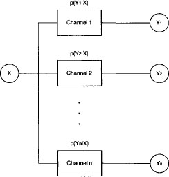
H.3* Instance 8.5 shows that Bayesian and maximum likelihood decoding establish optimization problems. This application only considers one channel. Identify the optimization problems that occur when multiple channels are connected in series as shown in Figure 8.3 and in parallel as shown in Figure 8.4.
Figure 8.3 A serial connection of unreliable, memoryless channels.
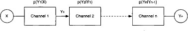
Figure 8.4 A parallel connection of unreliable, memoryless channels.
H.4** Context valuation algebras from Chapter 7 are based on the duality between the sentences of a language and their models. All instances of this family satisfy idempotency and can therefore be processed by the idempotent architecture of Section 4.5. In the introduction to this chapter, we mentioned several examples of context valuations as typical formalisms with some notion of solutions, i.e. solutions in linear equations, inequalities or models in different logics. Show that the set of models associated with a context valuation always satisfies the requirements for a solution set. Moreover, show that the interpretation of solution construction as local computation in the relational algebra of solution sets given in Section 8.2.1 and recessed in Exercise H.1 then complies with the usual distribute phase in the idempotent architecture. Finally, investigate property (8.9) for context valuation algebras.