
1
Stresses and Shear Strength of Soils
In the design of earth structures, good knowledge of shear stiffness/strength of soil is of importance because excessive deformation or failure of earth structures may occur as a result of insufficient resistance to shear stress. This chapter presents a review of shear behavior and shear strength of soils that are relevant to the design of earth structures. We begin the chapter with an explanation of stress at a point, followed by a brief explanation of effective stress and Mohr–Coulomb failure criterion. We then discuss commonly used laboratory and field tests for evaluation of shear behavior and determination of the shear strength of soils. We conclude the chapter with a discussion of the design consideration of the shear strength for soils under different loading conditions.
1.1 Stress at a Point
In engineering analysis and design of structures, stress has been proven to be an extremely useful parameter to quantify the effects of internal and external influences on a structure. For earth structures, common influences include external loads, self‐weight of soil and water, seepage force, and temperature change. Stress in a body is commonly referred to a plane. Stress on a plane with cross‐sectional area A when subjected to a force system denoted F can be evaluated by a simple equation: ![]() . This equation, however, is useful only if the force on the given plane is known and if the stress can be approximated as being uniform on that plane. This is generally not the case for a soil mass where the stresses of interest typically occur on a plane other than the plane of load applications, and the stresses may be far from being uniform. To this end, we shall begin the discussion with a review of the stress at a point, a subject we were first exposed to when studying “mechanics of materials” as undergraduate engineering students. We shall discuss three topics that will help us gain a better understanding of stresses at a point: (a) the concept of stress at a point in terms of stress vector, (b) the computation of stress vector on any given plane by the Cauchy formula, and (c) graphical representation of stress at a point by a Mohr circle and the pole of a Mohr circle. A good understanding of these topics will allow us to gain insights into Rankine analysis, a prevailing lateral earth pressure theory, which we will discuss in detail in Chapter 2.
. This equation, however, is useful only if the force on the given plane is known and if the stress can be approximated as being uniform on that plane. This is generally not the case for a soil mass where the stresses of interest typically occur on a plane other than the plane of load applications, and the stresses may be far from being uniform. To this end, we shall begin the discussion with a review of the stress at a point, a subject we were first exposed to when studying “mechanics of materials” as undergraduate engineering students. We shall discuss three topics that will help us gain a better understanding of stresses at a point: (a) the concept of stress at a point in terms of stress vector, (b) the computation of stress vector on any given plane by the Cauchy formula, and (c) graphical representation of stress at a point by a Mohr circle and the pole of a Mohr circle. A good understanding of these topics will allow us to gain insights into Rankine analysis, a prevailing lateral earth pressure theory, which we will discuss in detail in Chapter 2.
1.1.1 Stress Vector
Let us begin by considering an earth retaining wall subjected to concentrated and distributed loads over the “crest” (top surface of a wall), as shown in Figure 1.1(a). Figure 1.1(b) shows a plane cutting through the soil mass behind the wall at point P. The force acting over a very small area ΔA on the plane of cut surrounding point P is denoted ΔF. If the plan of cut is referred to as the “![]() plane” (i.e., a plane with its outward normal being a unit vector
plane” (i.e., a plane with its outward normal being a unit vector ![]() ; the arrow above the notation “n” is merely a symbol indicating that it is a vector, i.e., it has a magnitude, an orientation, and a sense), the intensity of force at point P on the
; the arrow above the notation “n” is merely a symbol indicating that it is a vector, i.e., it has a magnitude, an orientation, and a sense), the intensity of force at point P on the ![]() plane can be expressed by a stress vector
plane can be expressed by a stress vector ![]() as:
as:
Figure 1.1 (a) An earth retaining wall subjected to self‐weight and external loads on the crest and (b) stress resultant  on a plane
  through point P
Note that the stress vector can be viewed as the resultant of stresses on the ![]() plane.
plane.
We shall find it convenient to identify two major components of ![]() which are perpendicular and tangent to the
which are perpendicular and tangent to the ![]() plane:
plane:
The stress vector ![]() is therefore a resultant of normal stress σ and shear stress τ on the given plane.
is therefore a resultant of normal stress σ and shear stress τ on the given plane.
If we had chosen a different plane of cut through point P, the stress vector on that plane would generally be different from what we obtained previously. In fact, for every plane passing through point P, there will generally be a different stress vector associated with that plane. The number of planes passing through point P is infinite; hence, there are infinite stress vectors at point P. Stress at point P is the totality of all the stress vectors at point P. To state that we know the stress at a given point, we must know all the stress vectors at that point.
1.1.2 Cauchy Formula
Since there is an infinite number of stress vectors at a point, it would appear that it is not possible to know the stress at a point. This problem was resolved thanks to the Cauchy formula. Cauchy (circa 1820) showed that the stress vector on any plane at a point could be determined provided that the stress vectors on three orthogonal planes at that point are known, i.e.,
where
-
 = the stress vector on a plane with its outward normal unit vector
-
 = the stress vectors on the x‐, y‐, and z‐planes, respectively
 - nx , ny , nz = directional cosines of
 in the x‐, y‐, and z‐directions, respectively, where
  (see Figure 1.2).
Figure 1.2 Directional cosines of a plane with an outward normal unit vector 
The Cauchy formula, Eqn. (1‐2), allows the stress vectors on any plane to be determined by knowing only the stress vectors on three orthogonal planes; therefore, stress at a point can now be fully defined by knowing only the stress vectors on three perpendicular planes ![]() , and
, and ![]() . As shown in Figure 1.3,
. As shown in Figure 1.3, ![]() can be considered as the resultant of σx , τxz , and τxy. Similarly,
can be considered as the resultant of σx , τxz , and τxy. Similarly, ![]() can be considered as the resultant of σy , τyz , and τyx ; and
can be considered as the resultant of σy , τyz , and τyx ; and ![]() , the resultant of σz , τzx , and τzy.
, the resultant of σz , τzx , and τzy.
Figure 1.3 Stress vector  as the resultant of stress components σx , τxz , and τxy
Since the stress at a point can be defined completely by ![]() , and
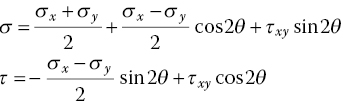
, and ![]() , it follows that the stress at a point can be described by nine stress components, known as the stress tensor:
, it follows that the stress at a point can be described by nine stress components, known as the stress tensor:
All of us may have seen a graph like Figure 1.4 in engineering mechanics books whenever the subject of stress comes up. The graph shows the nine components of the stress tensor, hence stress at a point. Even though the graph shows the nine components on a cube, we should picture it in our mind as a point. The cube is just a convenient way to show stresses on different planes. With an assumption that the body‐moment and couple‐stress do not exist in the system, the stress tensor must be symmetrical, i.e., ![]() (Fung, 1977). The stress tensor therefore has only six independent components.
(Fung, 1977). The stress tensor therefore has only six independent components.
Figure 1.4 Representation of stress at a point by a stress tensor
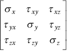
In a plane‐strain condition (see Section 1.4.3), a three‐dimensional structure can be analyzed as being two‐dimensional. Stress at a point in a plane‐strain condition is therefore fully defined if the stress vectors on two orthogonal planes at the point of interest are known (an extension of this statement can be seen in Examples 1.2 and 1.3). The stress tensor in a plane‐strain condition can be expressed as:

This stress tensor has three independent stress components (σx, σz, σxz). If these three stress components are known, stresses on any plane at the point can be determined by the Cauchy formula. For example, the normal stress (σ) and shear stress (τ) on a plane with an outward normal unit vector ![]() making an angle θ with the x‐axis (as shown in Figure 1.5) can be calculated by:
making an angle θ with the x‐axis (as shown in Figure 1.5) can be calculated by:
Eqn. (1‐3) is a simplified form of the Cauchy formula (Eqn. (1‐2)) in a two‐dimensional condition.
Figure 1.5 Two‐dimensional representation of a plane with its outward normal unit vector 
It should be noted that the use of the concept of stress in the analysis of earth structures is based on an assumption that soil is a continuum. Since soil is in fact a particulate material, in that the particles are typically not bonded and voids are always present, the assumption of a continuum maybe questionable (see Figure 1.6). However, we shall continue to make use of “stress” for the design and analysis of earth structures because it has proven to be an extremely useful tool. Keep in mind, however, that stress in soil is merely a “defined” parameter. When referring to stresses in a soil, it should be viewed on a macro‐scale, and the soil is considered a continuum for the purposes of engineering analysis.

Figure 1.6 Stress at a point in a soil mass: (a) reality (micro‐scale) and (b) idealized as being a uniform continuum (macro‐scale)
1.1.3 Mohr Circle of Stress
The Mohr circle of stress, as shown in Figure 1.7(a), is a plot of normal stress vs. shear stress of all permissible stresses at a point under two‐dimensional conditions. Every point on a Mohr circle represents the normal and shear stresses on a particular plane at that point. A Mohr circle of stress therefore can be regarded as a graphical representation of stresses at a point under two‐dimensional conditions. There are an infinite number of points on a Mohr circle, and each point corresponds to a plane passing through the point of interest. Two distinct planes exist on a Mohr circle where shear stress ![]() . These planes are called principal planes. The stresses on the principal planes are known as principal stresses, denoted by σ1 and σ3 , as shown in Figure 1.7(a). The principal stress σ1 is the largest normal stress (or major principal stress), whereas the principal stress σ3 is the smallest normal stress (or minor principal stress).
. These planes are called principal planes. The stresses on the principal planes are known as principal stresses, denoted by σ1 and σ3 , as shown in Figure 1.7(a). The principal stress σ1 is the largest normal stress (or major principal stress), whereas the principal stress σ3 is the smallest normal stress (or minor principal stress).
Figure 1.7 (a) Two‐dimensional representation of stress at a point by a Mohr circle of stress and (b) sign conventions of normal and shear stresses for plotting Mohr circles
Figure 1.7(b) shows the sign conventions for plotting a Mohr circle of stress. In soil mechanics, we denote compressive normal stress as positive and tensile normal stress as negative, which is opposite to the sign convention commonly used in structural mechanics. We do so because soil has little tensile resistance, and most normal stresses in geotechnical engineering analysis are compressive. The sign convention of considering compressive stress as positive avoids having to show nearly every normal stress in geotechnical engineering analysis with a negative sign. A shear stress that makes a clockwise rotation about any point outside of the plane is considered a positive shear stress (see Figure 1.7(b)). Conversely, a shear stress making counterclockwise rotation about any point outside of the plane is considered a negative shear stress.
1.1.4 Pole of Mohr Circle
We recall that every point on a Mohr circle (with coordinates σ and τ) corresponds to a given plane at the point of interest. It would be very useful to associate the stresses σ and τ with the plane. To that end, the pole of planes (or simply pole) of a Mohr circle is the most useful. The pole, also referred to as the origin or center of planes, is a unique point on a Mohr circle that allows us to determine the orientation of the plane for a given set of permissible σ and τ; it also allows us to determine σ and τ on any given plane.
Once the pole of a Mohr circle is located, we can connect the pole with any point on the circle by a straight line; the orientation of the straight line is then the orientation of the plane. Take a point of coordinates (σa, τa) on a Mohr circle shown in Figure 1.8(a), for example. The orientation of the plane on which stresses σa and τa act is indicated by a straight line connecting the pole with point (σa, τa). Figure 1.8(b) shows the orientation of the two planes of maximum shear stress, each determined by a straight line connecting the pole with the point on the Mohr circle having the largest magnitude of τ. There is one unique plane denoted by a line tangent to the Mohr circle at the pole. The orientation of that tangent line is the orientation of the plane on which the stresses σpole and τpole act.
Figure 1.8 (a) The pole of a Mohr circle of stress and (b) orientation of planes of maximum shear stress
The only question remaining is: how do we locate the pole of a Mohr circle? The answer is simple. There is one and only one pole for each Mohr circle. Therefore, if one permissible set of stress (σa and τa) and the orientation of the plane of (σa, τa) are known, the pole can be located by back‐tracking the step described above. In other words, all we have to do is draw a straight line through point (σa, τa) parallel to the given orientation to the plane; the pole of the Mohr circle is the point where the line intersects the Mohr circle. Example 1.1 illustrates how the pole of a Mohr circle of stress is determined. Since σ = 5 psi and τ = 2 psi (denoted by point A on the Mohr circle) are known to act on the vertical plane, a vertical line can be drawn through point A to locate the pole of the Mohr circle. Note that the pole can also be located by the stresses on the horizontal plane, σ = 1.5 psi and τ = –2 psi. Again, there is only one pole for a Mohr circle, so the location of the pole as determined by any sets of σ and τ will be the same. Note that the orientation of a plane deduced from a pole reflects the actual orientation of the plane. The orientation can be described by an angle that it makes with the horizontal, the vertical, or any other reference plane.
Examples 1.2 and 1.3 provide additional exercises on how the concept of pole can be used to determine stresses on a plane.
1.2 Concept of Effective Stress
Natural soil is generally a three‐phase material, comprising solid particles, pore water, and pore air. Since the pore fluids (pore water and pore air) offer no resistance to static shear stress, the conventional definition of stress has to be revised when dealing with the shear strength of soil. This brings about the concept of effective stress. The effective normal stress, commonly denoted as σ', is the part of applied normal stress that controls the shear resistance and volume change of a soil when water is present in the pores. In 1923, Terzaghi presented the principle of effective stress, an intuitive relationship based on experimental data of fully saturated soils. The relationship is:
where σ is the total stress and u is the porewater pressure. The total stress is the stress calculated by picturing the soil as a single‐phase continuum, i.e., the definition commonly used for normal stress.
Although the shear resistance of soil is controlled by effective stress, it is sometimes simpler to perform stability analysis of earth structures in terms of total stress because it does not require us to know the porewater pressure. This, however, is only warranted when a valid relationship can be established between shear strength and total stress. Such a relationship is only available in a limited number of cases where variations of in situ porewater pressure or drainage conditions do not deviate significantly from those in the laboratory tests. The short‐term stability of saturated clays is a distinct example where total stress analysis with undrained shear strength can be carried out for stability analysis. This point will be addressed further in Section 1.5.2.
1.3 Mohr–Coulomb Failure Criterion
If shear stress on a plane reaches a limiting maximum value on that plane, shear failure is said to occur. A number of failure criteria for soils have been proposed to define the limiting condition, such as Mohr–Coulomb criterion, triangular conical criteria, extended von Mises criteria, curved extended von Mises criteria (Lade, 2005). Among these failure criteria, the first two have frequently been used for analysis of earth structures conducted by the finite element methods of analysis. The Mohr–Coulomb failure criterion is by far the most commonly used criterion for limiting equilibrium analysis and routine design of earth structures.
In the Mohr–Coulomb failure criterion, the shear strength (τf ) of soil can be described by the following equation:
in which σf is normal stress at failure, ϕ is the angle of internal friction (or simply friction angle), and c is cohesion. Even though Eqn. (1‐5) is a common expression of the Mohr–Coulomb failure criterion, it falls short of describing the stresses involved in a rigorous manner. We know from Section 1.1 that stresses are generally different on different planes. However, Eqn. (1‐5) only describes the relationship between the normal and shear stresses at failure, and does not address the associated plane of the stresses. Yet it has been found to be a useful expression for performing total stress analysis in which the strength of a soil is defined by total stress strength parameters c and ϕ. This point is discussed further in Section 1.5.
A more rigorous expression of Mohr–Coulomb failure criterion is given in terms of effective stress as:
In Eqn. (1‐6), the double subscript ff denotes on failure plane at failure, τff is the shear stress on failure plane at failure (commonly referred to as shear strength), ![]() is the effective normal stress on failure plane at failure, and c′ and ϕ′ are effective shear strength parameters. Recall Terzaghi’s effective stress principle that the shear resistance of soil is dictated by effective stress, as seen in Eqn. (1‐6).
is the effective normal stress on failure plane at failure, and c′ and ϕ′ are effective shear strength parameters. Recall Terzaghi’s effective stress principle that the shear resistance of soil is dictated by effective stress, as seen in Eqn. (1‐6).
As shown in Figure 1.9, the straight line given by Eqn. (1‐6) is a line tangent to all effective stress Mohr circles at failure. Failure is said to occur when the Mohr circle “touches” the straight line, known as the Mohr–Coulomb failure envelope. The point of tangency (such as point F in Figure 1.9) represents the effective normal stress and shear stress on failure plane at failure. Note that this is true only when the normal stress is expressed in terms of effective stress. Also note that the failure envelopes for many soils may not necessarily be straight lines, especially for dense soils (dense sands and stiff clays), but a straight‐line approximation can be taken over the range of stress of interest. This is discussed further in Section 1.5.1.
Figure 1.9 The Mohr–Coulomb failure criterion in terms of effective stress, where stresses on the failure plane at failure (σff', τff) are represented by the point of tangency of the Mohr circle
In terms of principal stresses, the Mohr–Coulomb failure criterion can be expressed as
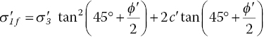
or
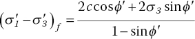
The subscript f in Eqns. (1‐7) and (1‐8) means “at failure.” These equations are useful in some applications of the Mohr–Coulomb failure criterion.
The use of the Mohr–Coulomb failure criterion requires determination of the Mohr–Coulomb strength parameters c' and ϕ' (or c and ϕ). It is important to keep in mind that these strength parameters are not “inherent” soil properties. Their values have been found to vary with the drainage condition, stress path, and stress history of a soil.
1.4 Shear Strength Tests
We will now look at some common tests used for determining the shear strength of soils, with emphasis on determination of the Mohr–Coulomb shear strength parameters c' and ϕ' (referred to as Mohr–Coulomb drained strength parameters) or c and ϕ (referred to as Mohr–Coulomb undrained strength parameters). The shear strength parameters can be determined by conducting laboratory tests or in situ (a Latin phrase meaning “on site”) tests. The most commonly used laboratory tests are the direct shear test, the triaxial compression test, and the unconfined compression test. The most common field tests in North America are the standard penetration test and the cone penetration test. For cohesive soils, vane shear tests have sometimes been used in the laboratory as well as in the field for determination of undrained shear strength.
There is an abundance of literature on shear strength tests (e.g., Bishop and Henkel, 1962; Head and Epps, 1982; Holtz et al., 2011). Only a brief description of commonly used shear strength tests is given here.
1.4.1 Direct Shear Test
Figure 1.10 shows a schematic diagram and a photo of direct shear test setup and apparatus. In direct shear test, a specimen of soil prepared at prescribed density and moisture content is confined laterally in a metal box of a square or circular cross‐section. The box is split horizontally in half with a small clearance between the upper and lower boxes. The test is typically carried out by fixing the position of the lower box and applying horizontal forces to move the upper box relative to the lower box. A constant normal load (N) is first applied to the top of the specimen by a dead weight or an air bladder, then the shear force (T) exerted on the upper box is gradually increased until failure occurs. The test is usually repeated with a few different normal loads to determine the Mohr–Coulomb strength parameters c and ϕ.

Figure 1.10 Direct shear test: (a) schematic test setup and (b) a photo of test apparatus
A typical set of direct shear test results are shown in Figure 1.11(a). In addition to the relationships between the relative displacements of the upper and lower boxes (δ) and the shear stress (![]() ), vertical displacement of the soil specimen during shear is often measured as well. By plotting the relationship between the shear stress at failure (τf
), vertical displacement of the soil specimen during shear is often measured as well. By plotting the relationship between the shear stress at failure (τf![]() ) vs. the corresponding normal stress (
) vs. the corresponding normal stress (![]() ), as shown in Figure 1.11(b), the Mohr–Coulomb failure envelope of the soil can be obtained. The failure envelope is formed by simply drawing a best‐fit straight line through the data points. Unlike in triaxial tests (see Section 1.4.2), there is no need to sketch Mohr circles at failure and find the common tangent of the circles in this case. This is because the data points, such as those shown in Figure 1.11(b), are stresses on the failure plane (the horizontal plane in this case) at failure. Clean cohesionless soils have c = 0. For moist cohesionless soil or soil containing some fines, however, the best‐fit straight line failure envelope will likely have a non‐zero intercept (i.e., cohesion, c ≠ 0). This cohesion is called apparent cohesion and should be ignored in design as it cannot be counted on during the service life of an earth structure.
), as shown in Figure 1.11(b), the Mohr–Coulomb failure envelope of the soil can be obtained. The failure envelope is formed by simply drawing a best‐fit straight line through the data points. Unlike in triaxial tests (see Section 1.4.2), there is no need to sketch Mohr circles at failure and find the common tangent of the circles in this case. This is because the data points, such as those shown in Figure 1.11(b), are stresses on the failure plane (the horizontal plane in this case) at failure. Clean cohesionless soils have c = 0. For moist cohesionless soil or soil containing some fines, however, the best‐fit straight line failure envelope will likely have a non‐zero intercept (i.e., cohesion, c ≠ 0). This cohesion is called apparent cohesion and should be ignored in design as it cannot be counted on during the service life of an earth structure.
Figure 1.11 Results of direct shear tests under three normal loads: (a) relationship between relative displacement (δ) and shear stress (τ), and (b) relationship between normal stress (σn) and shear stress at failure (τf); all stresses are on the failure plane (the horizontal plane)
For sands in a dense condition, the relationship between relative displacement (δ) and shear stress (τ) typically shows a “drop” after a peak value of τ is reached, and reduces to a residual value (see Figure 1.12(a)). This behavior is termed softening. In such a case, friction angles corresponding to peak strength and residual strength can be obtained. Note that the initial area (A), rather than corrected shear areas occurred during testing, is usually used in the calculations of σn and τf . This is because the ϕ‐value is little affected by the use of the corrected area. The former is usually larger than the latter. In some cases, the reverse can occur; i.e., ϕresidual > ϕpeak , as seen in Figure 1.12(b). This is due to the difference in apparent cohesion, which can be larger for the peak strength than for the residual strength. For design purposes, ϕpeak should usually be used. If large deformation due to progressive failure is expected, ϕresidual should be used instead.

Figure 1.12 Direct shear test results: (a) peak and residual strengths, and (b) failure envelopes of peak and residual strengths (for some soils, ϕresidual may be larger than ϕpeak , as shown)
1.4.2 Triaxial Test
Most triaxial tests are performed by applying vertical axial loads to a cylindrical soil specimen while it is subjected to pressure confinement. The setup and a photo of triaxial test are shown in Figure 1.13. In a triaxial test, a cylindrical soil specimen is fitted between two rigid end caps, with its vertical surface covered by a flexible latex membrane, placed inside an enclosed cell/chamber that is filled with water (although air pressure, positive or negative, can also be used), and loaded vertically until failure occurs.
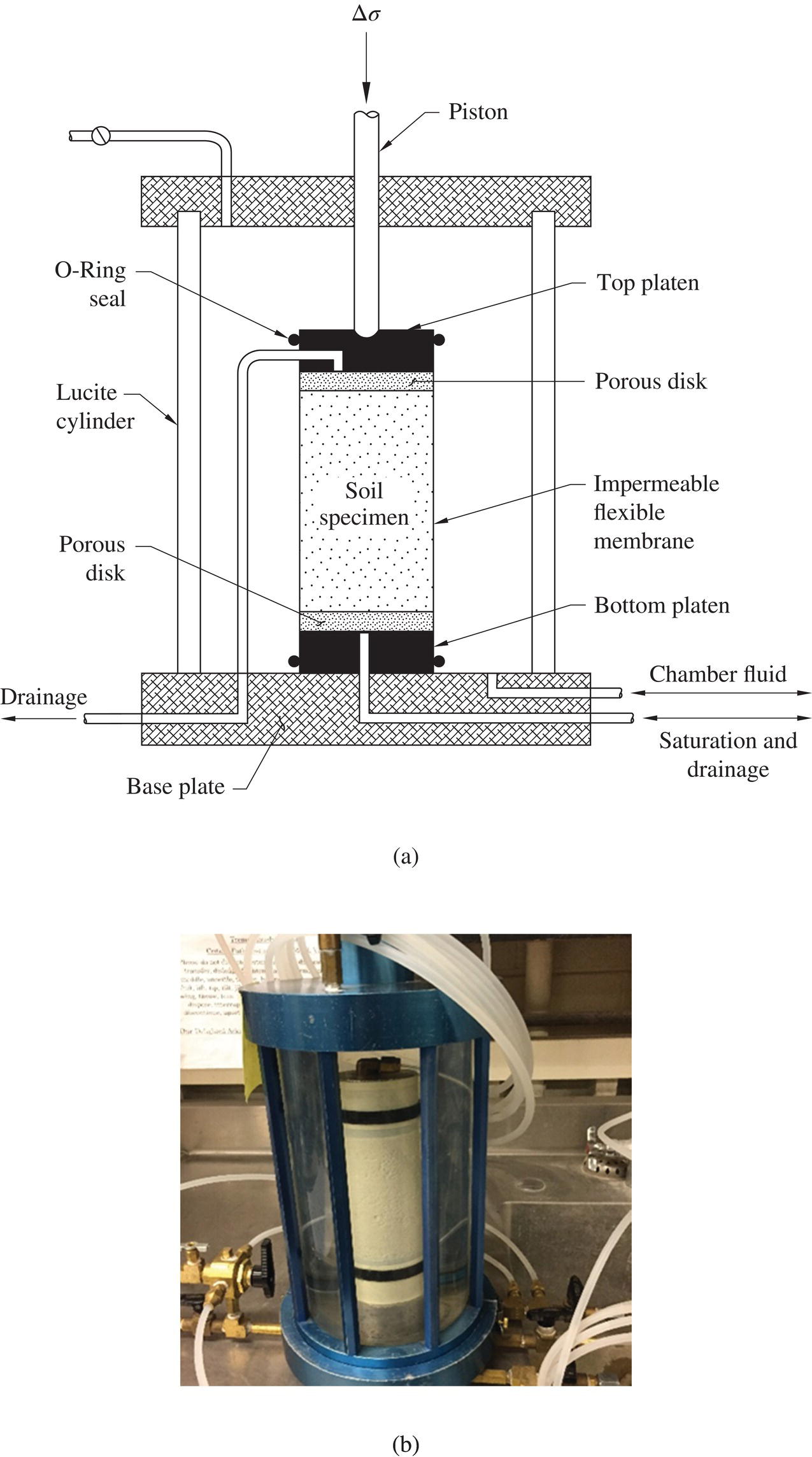
Figure 1.13 Triaxial test: (a) schematic test setup and (b) a photo of test specimen and test apparatus
A triaxial test is conducted in two stages. In stage 1, cell pressure (or confining pressure) is applied to the cylindrical soil specimen to provide pressure confinement (and consolidate the specimen if a consolidated triaxial test is performed). In stage 2, increasingly larger vertical axial compressive loads are applied to the specimen through a piston connected to the top of specimen until failure occurs. Triaxial tests with this mode of loading are referred to as axial compression triaxial tests.
Figure 1.14 shows Mohr circles corresponding to the two stages of a triaxial test. In stage 1, the soil specimen is subjected to an equal cell pressure (σc ) in all directions, the corresponding Mohr circle is simply a point on the σ‐axis, and the soil is not subject to any shear stress on any plane; the soil specimen is said to be subject to hydrostatic loading (in stage 1). In stage 2, however, the Mohr circle becomes a circle, and the circle will grow larger in size as increasing vertical load is applied. Other than the principal planes, all other planes are subjected to shear stress of different magnitudes; the soil specimen is said to be subject to shear (in stage 2).
Figure 1.14 Mohr circles of an axial compression (AC) triaxial test: (a) stage 1 (hydrostatic loading) and (b) stage 2 (shear)
Figure 1.15 depicts schematically the results of triaxial tests conducted by using different confining pressures, high, medium, and low. The upper part of the figure shows stress–strain relationships in stage 2 (shear) loading, plotted in terms of change in axial stress versus change in axial strain. The change in axial stress is commonly expressed in terms of deviator stress which is the difference in principal stresses ![]() versus the change in axial strain which is the change in vertical strain (ε1 or εvertical). As seen in Figure 1.15, the stiffness (i.e., the slopes of the stress–strain curves) and strength of the soil are usually higher under larger consolidation/confining pressure. The lower part of Figure 1.15 shows the change in volumetric strain εv (in a drained test) or the change in porewater pressure u (in an undrained test). In a drained test, most soils would exhibit compression (reduction in volume) at small axial strains, follow by dilation (increase in volume) as strain increases. In an undrained test, volume change is prohibited, hence the “tendency” for volume change is reflected by change in porewater pressure. A tendency of dilation is reflected by a decrease in porewater pressure, and a tendency of compression by an increase in porewater pressure.
versus the change in axial strain which is the change in vertical strain (ε1 or εvertical). As seen in Figure 1.15, the stiffness (i.e., the slopes of the stress–strain curves) and strength of the soil are usually higher under larger consolidation/confining pressure. The lower part of Figure 1.15 shows the change in volumetric strain εv (in a drained test) or the change in porewater pressure u (in an undrained test). In a drained test, most soils would exhibit compression (reduction in volume) at small axial strains, follow by dilation (increase in volume) as strain increases. In an undrained test, volume change is prohibited, hence the “tendency” for volume change is reflected by change in porewater pressure. A tendency of dilation is reflected by a decrease in porewater pressure, and a tendency of compression by an increase in porewater pressure.
Figure 1.15 Results of axial compression triaxial tests under different confining pressures
One major advantage of the triaxial test over the direct shear test is that the drainage condition of the soil specimen during testing can be controlled to simulate the drainage condition anticipated in the field; also, porewater pressure during testing can be measured in an undrained test. Three common types of triaxial tests for different drainage conditions are the unconsolidated undrained (UU) test, the consolidated undrained (CU) test, and the consolidated drained (CD) test. The first word of these terms (either U or C) refers to stage 1 testing; namely, whether drainage (consolidation) is allowed in stage 1 of triaxial testing while the soil specimen is being subjected to a prescribed confining pressure. The second word (either U or D) refers to stage 2 of testing; namely, whether drainage is permitted during application of deviator stress.
Assuming that vertical stress and confining pressure are principal stresses (denoted by σ1 and σ3), soil strength parameters c' and ϕ' (or c and ϕ) can readily be determined from the principal stresses at failure in triaxial tests. Example 1.4 illustrates how the effective strength parameters c' and ϕ' are determined from the results of three consolidated drained (CD) triaxial tests. The example also shows how the orientation of failure planes is determined with the aid of Mohr circles.
The shear strength of a soil in a drained condition is usually quite different from that in an undrained condition. A drained condition is usually assumed for soils of high permeability in that the excess porewater pressure induced by applied loads will dissipate quickly without accumulation. On the other hand, an undrained condition is usually assumed for soils of low permeability immediately after load applications before any significant consolidation can take place. (Note: the term consolidation refers to “deformation accompanied by dissipation of porewater pressure”.) Low‐permeability soils in the field typically change gradually from an undrained condition to a drained condition after load applications. When consolidation is eventually completed, shear strength of low‐permeability soils will become drained strength. The drained strength of a soil can be expressed in terms of effective stress with shear strength parameters c′ and ϕ′. The undrained strength, on the other hand, can be expressed in terms of total stress, with shear strength parameters cu and ϕu (or simply denoted as c and ϕ).
The drained strength of a soil may be obtained by performing either drained tests or undrained tests. If an undrained test is used, the effective stress can be computed by simply subtracting measured porewater pressure from the applied (total) stress if the soil is fully saturated. Example 1.5 shows how drained strength parameters (c′ and ϕ′) and undrained strength parameters (c and ϕ) of a saturated clay can be determined from results of CU triaxial tests with measured porewater pressure. Loose sands and normally consolidated clays typically have positive porewater pressure at failure, whereas dense sands and overconsolidated clays typically have negative porewater pressure at failure. The behavior for a loose sand to contract and a dense sand to dilate during shear is explained by Leonards (1962) using the sketches shown in Figure 1.16.
Figure 1.16 Conceptual volume change behavior during shear of loose sand and dense sand (Leonards, 1962)
Figure 1.17 shows idealized failure envelopes of typical loose sand, dense sand, normally consolidated clay, and overconsolidated clay, in terms of both total and effective stresses. The strength parameters c = c' = 0 as determined in Example 1.5 suggest that the clay in the example is normally consolidated. It is important to point out that failure envelopes are usually curved (concave downward) for dense sands and overconsolidated clays. This point is addressed further in Section 1.5.
Figure 1.17 Idealized failure envelopes of (a) loose sand, (b) dense sand, (c) normally consolidated clay, and (d) overconsolidated clay (compare with Figures 1.29 and 1.35 in Section 1.5 for nonidealized dense sand and overconsolidated clay, respectively)
The stress–strain behavior and volume change (or porewater pressure change) behavior of a soil is significantly affected by its initial state. Figure 1.18 shows comparative triaxial test results of loose sand/normally consolidated clay, medium sand/lightly overconsolidated clay, and dense sand/heavily overconsolidated clay. Dense sands and heavily overconsolidated clays usually show strain softening, i.e., a peak deviator stress is reached then reduces to a residual value. For loose sands and normally consolidated clays, on the other hand, a peak deviator stress is usually reached at failure with little or no strain softening. In terms of volume change (in a drained test) and porewater pressure change (in an undrained test), dense sands and heavily overconsolidated clays usually show dilation (in a drained test) or negative porewater pressure (in an undrained test) at failure, whereas loose sands and normally consolidated clays usually show contraction (in a drained test) or positive porewater pressure (in an undrained test) at failure.
Figure 1.18 Comparative results of axial compression triaxial test for loose to dense sands, and normally consolidated to overconsolidated clays (modified after Japanese Foundation Engineering Society, 1995)
In addition to being able to control drainage conditions during testing, a triaxial test can also control the loading path to simulate the anticipated loading conditions of an earth structure. Figure 1.19 shows four loading paths that can be simulated by a triaxial test. Also shown is an example application of each loading path. The loading paths are axial compression (AC), lateral extension (LE), axial extension (AE), and lateral compression (LC). Our discussions thus far have been focused on AC, even though other loading paths may be more applicable to a certain loading condition. Note that AC and LE tests make a specimen shorter and wider, and AE and LC will have the opposite effect, making a specimen longer and narrower. The results of AC and LE tests for most soils have been found to be nearly identical, and so have the results of AE and LC tests. The ϕ'‐value measured from triaxial AE and LC tests is generally slightly higher than from AC and LE tests (typically about 10% higher for cohesionless soils, and about 20% higher for normally consolidated cohesive soils) (Kulhawy and Mayne, 1990). In some instances, however, the strength obtained from AE and LC tests of normally consolidated clays have been found to be much lower than those from AC and LE tests because of soil anisotropy (Hunt, 1986).
Figure 1.19 Loading paths of triaxial tests and example applications (modified after Holtz et al., 2011)
1.4.3 Plane‐Strain Test
A plane‐strain condition prevails if the geometry, material properties, and loads do not vary along the longitudinal direction of a very long structure. When the longitudinal dimension of a structure is about 10 times or greater than other dimensions, it is generally considered very long. Figure 1.20 shows examples of earth structures that can be approximated as being in a plane‐strain condition. For a structure in a plane‐strain condition, the longitudinal strain is equal to zero and there is no variation of stress or displacement in the longitudinal direction. Therefore, analysis of a structure in a plane‐strain condition can be performed by considering only a slice of the structure of unit thickness; i.e., a two‐dimensional analysis is applicable.
Figure 1.20 Examples of plane‐strain condition in which the longitudinal dimension of the structure (in the z‐direction) is much greater than other dimensions; also, there is no variation in geometry, material properties, or loading in the longitudinal direction
A plane‐strain test gives better simulation of many “long” earth retaining structures than a triaxial test. Figure 1.21(a) shows the setup of a test specimen in a plane‐strain test, in which a cuboidal soil specimen is confined between two lubricated rigid (acrylic/plexiglass) plates maintained a fixed distance apart. The soil‐plate assembly is then placed inside a pressure cell similar to that used in a triaxial test. The rigidity of the plates restrains the deformation of the soil specimen in the longitudinal direction to ensure zero longitudinal strain (εz = 0), while the lubricated surface allows the soil specimen to deform without artificial constraint on deformation in the other two directions. Tatsuoka et al. (1984) have developed a lubrication technique that is shown to result in an interface friction angle on the order of 0.05° at the contact surfaces of soil and a smooth plate (plexiglass). The technique, shown in Figure 1.21(b), involves introducing a latex membrane between the soil and the plexiglass, and applying a thin layer of silicon lubricant over the surface of the plexiglass. As seen in Figure 1.21(c), internal movement of the soil specimen can be monitored with very good accuracy by tracking the movement of a grid system printed on the latex membrane before testing.

Figure 1.21 Plane‐strain test: (a) schematic setup of test specimen, (b) a lubrication technique at the contact surface between soil and plexiglass developed by Tatsuoka, and (c) use of the lubrication technique to monitor internal movement of a soil specimen (photo courtesy of Hoe Ling)
Laboratory tests performed on medium and dense sands have indicated that the internal friction angle (ϕ′) determined by plane‐strain tests is approximately 10% higher than those determined by triaxial compression tests. For design of earth retaining walls, friction angles determined from triaxial tests are often used even when a wall is approaching a plane‐strain condition. The use of such friction angles would provide an added safety margin in design.
1.4.4 Vane Shear Test
The vane shear test is a testing method for determination of the undrained shear strength of non‐fissured, fully saturated clays. The vane shear test involves pushing a four‐bladed vane (see Figure 1.22) on the end of a rigid rod into the soil, then rotating the rod at 6–12° per minute until a cylinder of soil (diameter d, length h) contained within the blades is sheared off. By measuring the torque T required to induce failure of a soil, the undrained shear strength of the soil Su can be evaluated as:
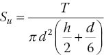
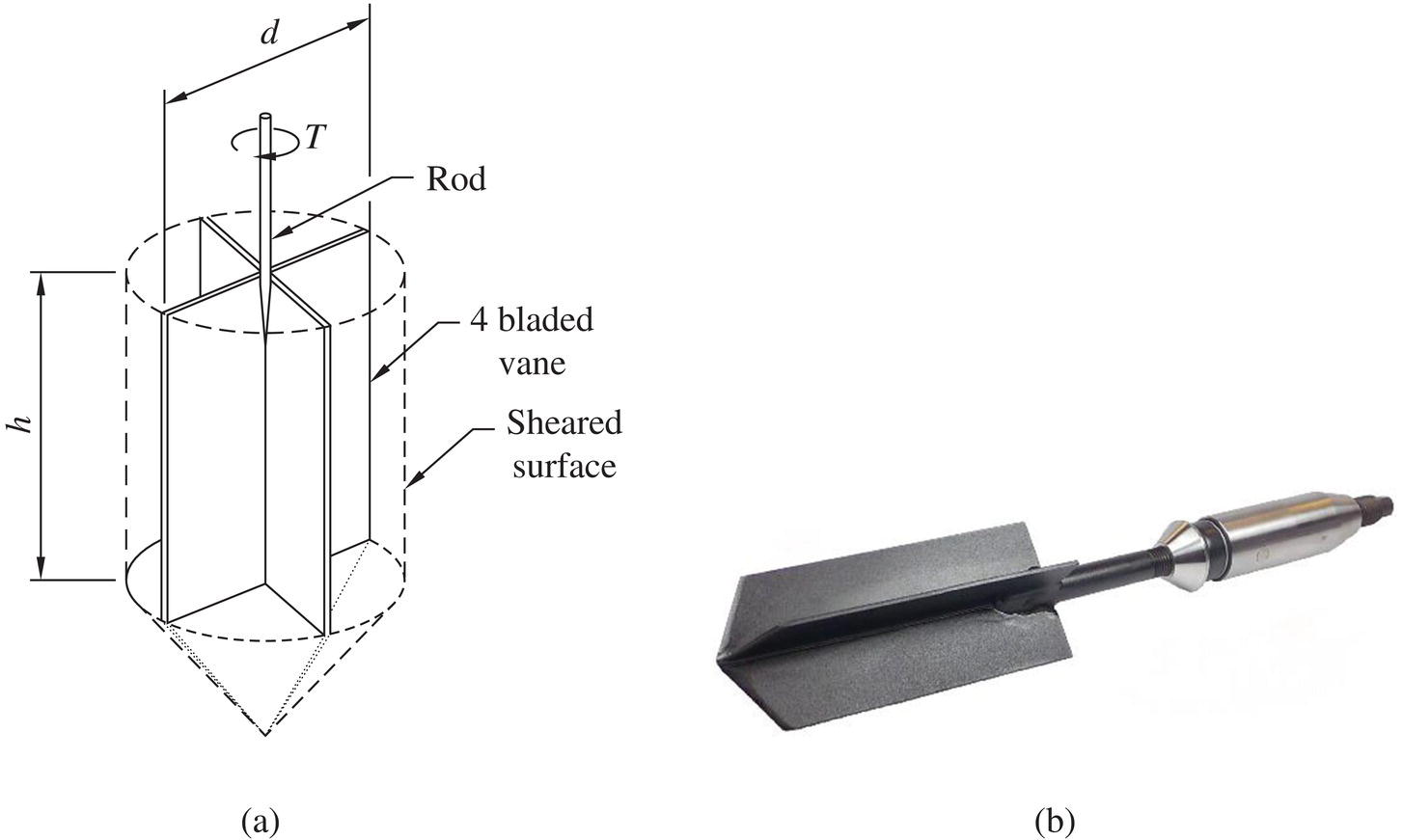
Figure 1.22 (a) Schematic diagram of a vane shear test and (b) photo of an electric vane (photo courtesy of Gouda Geo‐Equipment B.V., the Netherlands)
The vane shear test has been performed the in the field and in the laboratory. The former is typically performed in conjunction with drill‐hole explorations in soft to medium clays. The test can also be carried out in soft soil without a bore hole, by direct penetration of the vane from the ground level.
1.4.5 Standard Penetration Test
The standard penetration test (SPT) is the most widely used field test in North America. It is usually conducted as part of soil boring operations. The test involves lowering a standard size split‐spoon sampler (Figure 1.23(a)) to the bottom of a bore hole, and using a hammer weighing 140 lb (0.62 kN) free‐falling 30 inches to advance the sampler deeper into the ground (see Figure 1.23(b)). The number of blows of the hammer required to advance the split‐spoon sampler three successive 6‐inch (152‐mm) intervals into the bottom of the bore hole is recorded. The number of blows for the last 12 inches (305 mm) is termed the standard penetration resistance or blow count, commonly denoted by N.
Figure 1.23 The standard penetration test (SPT): (a) schematic diagram of a split‐spoon sampler and (b) typical SPT setup (Kovacs et al., 1981)
A number of relationships between N and shear strength have been suggested. The relationships for large gravels and clays are generally unreliable and can serve only as a reference. A simple yet rather reliable empirical correlation between N and ϕ′ for sands is shown Figure 1.24(a). This relationship has been used widely in routine geotechnical engineering design. A commonly used correlation between N and unconfined compressive strength, Uc (Uc = 2 Su for saturated clays, Su = undrained shear strength) for cohesive soils of low to high plasticity is shown in Figure 1.24(b).

Figure 1.24 Correlations between SPT blow count N and (a) angle of internal friction ϕ' of granular soils and (b) unconfined compressive strength Uc of cohesive soils (NAVFAC, 1986)
Studies have suggested that hammer efficiency (η) can vary over a wide range (30–90%), depending on the hammer type. Seed et al. (1985) and Skempton (1986) proposed that raw field N‐values be standardized to N60 to reflect η = 60%. This has become common practice. When not stated specifically, the N‐values in most correlations may be taken as being N60.
1.4.6 Cone Penetration Test
Estimation of the shear strength of a soil under static loading by means of a pseudo dynamic test, such as the standard penetration test, is inherently difficult, especially when free water level is encountered. More reliable estimation may be obtained from static penetration tests, of which the most commonly used in North America is the cone penetration test (CPT).
In the cone penetration test, a penetrometer with a cone‐shaped tip attached to a string of solid rods running inside hollow outer rods is pushed into the ground at a controlled rate. Figure 1.25 shows an overview of CPT testing with a truck‐mounted rig. Using the weight of the truck as reaction, a hydraulic ram located inside the truck pushes the cone into the ground. The end resistance of the cone at a given depth is recorded as the cone resistance, qc , and ![]() . After qc is determined, the outer rods are pushed downward. The cone and sleeve thus advance together after the range of motion inside the cone has been taken up. Such a sequence allows end bearing resistance and side friction to be determined separately. In some cone penetrometers (e.g., electric cones), a load cell is mounted near the conical tip and allows continuous recording of cone resistance. Other cone penetrometers, referred to as piezocones, can also measure porewater pressure at the conical tip.
. After qc is determined, the outer rods are pushed downward. The cone and sleeve thus advance together after the range of motion inside the cone has been taken up. Such a sequence allows end bearing resistance and side friction to be determined separately. In some cone penetrometers (e.g., electric cones), a load cell is mounted near the conical tip and allows continuous recording of cone resistance. Other cone penetrometers, referred to as piezocones, can also measure porewater pressure at the conical tip.
Figure 1.25 Overview of the cone penetration test (CPT) (Mayne, 2007)
A set of CPT test results is shown in Figure 1.26. The variation of cone resistance with soils of different types is evident from the cone resistance data. Various theoretical and empirical correlations have been developed to relate qc to ϕ′ for sands. One such correlation is given in Figure 1.27. For cohesive soils, correlations between qc and undrained shear strength (Su) have also been proposed. Sanglerat (1972) suggests Su = qc /15 for soft to stiff clays, and Su = qc/30 for stiff fissured clays. Schmertmann (1978) proposes the following correlation:
where Σ γ z = total overburden pressure at depth z and Nc = a correction factor (10 for stiff clays and 16 for soft clays with a Fugro friction cone).
Figure 1.26 A set of cone penetration test (CPT) data: cone resistance vs. depth with soil boring log (Mayne, 2007)

Figure 1.27 Correlations between cone resistance, overburden pressure, and internal friction angle (Robertson and Campanella, 1983)
A major disadvantage of CPT as compared with SPT is that soil samples are not obtained as part of the CPT test operations.
1.4.7 Plate Load Test
The behavior of a clay is known to be significantly affected by the stress history of the clay. The degree of prestress in a clayey deposit can be determined by performing a laboratory consolidation (oedometer) test on undisturbed field samples. The engineering behavior of granular soils is also affected strongly by the stress history. A granular soil that has been prestressed is known to be much stronger than the same soil in a non‐prestressed state. Since undisturbed field samples of granular soils are extremely difficult to obtain, the degree of prestress in a granular soil deposit needs to be determined by in situ tests. Among the many in situ shear tests, the plate load test is among the few methods that can capture directly the extent of prestress in a granular deposit.
The setup of a plate load test is shown in Figure 1.28(a), which involves applying increasing vertical loads to a 1‐ft diameter circular plate (or 1 ft × 1 ft square plate) on the bottom of a test pit and recording the accompanied settlement. The load–settlement curves for non‐prestressed sands (under drained conditions) of different N‐values have been established by Leonards (personal communication, circa 1978), as shown in Figure 1.28(b). By sketching the load–settlement curve obtained from an actual plate load test conducted on a granular deposit and comparing it with the curves in Figure 1.28(b), the level of prestress of the granular deposit can be estimated. For example, Figure 1.28(c) shows the load–settlement curve obtained from an actual plate load test performed on a sand with an SPT blow count of 4. A comparison of the load–settlement curve for non‐prestressed sand of N = 10 reveals that the soil in this case has been prestressed to approximately 0.8 tons/ft2. The level of prestress will affect the settlement significantly in response to applied loads. Prevailing methods for predicting settlement in sands (e.g., methods proposed by Terzaghi and Peck, 1967; Peck et al., 1974; Schmertmann, 1978) are all for non‐prestressed sands. In this example, for loads ranging between 0 and 0.8 tons/ft2, the corresponding settlement can be conservatively estimated as about 1/5 of that of the non‐prestressed sand. On the other hand, for the part of the load exceeding 0.8 tons/ft2, the corresponding settlement is that of the non‐prestressed sand.

Figure 1.28 The plate load test: (a) schematic test setup, (b) “the” load–settlement curves for non‐prestressed sands in a drained condition (Leonards, circa 1978), and (c) a measured load–settlement curve from an actual plate load test vs. the load–settlement curve of non‐prestressed sand for N = 10 (Leonards, circa 1978)
1.5 Design Considerations
1.5.1 Shear Strength of Granular Soils
When a granular soil is subjected to static loads, pore water would typically drain rapidly with little build up of excess porewater pressure due to high permeability; therefore, drained strength generally prevails in design. As granular soil has little or no cohesion (c′ = 0), the shear strength of sands or gravels is typically characterized only by the Mohr–Coulomb strength parameter ϕ′, the effective angle of internal friction. In practice, it is often referred to as ϕ (without a prime) for simplicity, but the friction angle of granular soils always means the effective friction angle for granular soils.
The value of ϕ′ of a granular soil can be determined by performing laboratory tests, such as the direct shear test, triaxial test, plane‐strain test, etc. For triaxial tests, CU tests (with porewater pressure measurement) or CD tests may be performed. For a given granular soil, the value of ϕ′ determined by direct shear tests is generally slightly lower than that by triaxial tests, which in turn is generally slightly lower than that by plane‐strain tests. When performing these laboratory tests, large particles will need to be removed prior to testing. Large particles are those larger than about 1/10 of the specimen diameter for triaxial tests, and about 1/6 of the specimen diameter (or the side of a square specimen) for direct shear tests. Note that when preparing laboratory test specimens with large particles removed, it is the relative density of the in situ soil that should be replicated, not the void ratio.
If a granular soil is indeed cohesionless (i.e., without appreciable amount of fines, say more than 5–10%, which are “sticky when wet”), proper data interpretation for determination of ϕ' is to find the best‐fit straight line through the data points or tangent to Mohr circles at failure and ignore the cohesion intercept, rather than forcing a straight line through the origin, even though the cohesion is known to be zero. The Mohr–Coulomb failure envelope of compacted granular soils is generally curved over a range of lower normal stress, as seen in Figure 1.29; the denser the soil, the more “curved” the failure envelope in that range. For design purposes, a secant value over the range of relevant normal stress could be used. Example 1.6 illustrates this procedure.
Figure 1.29 Mohr–Coulomb strength envelopes of compacted granular soils; the denser the soil, the more curved the strength envelope
An alternative approach to plotting Mohr circles at failure for determination of the strength parameters c' and ϕ' is to make use of a p–q diagram. In this approach, the values of ![]() and
and ![]() at failure are calculated and plotted as shown in Figure 1.30. After a best‐fit straight line is drawn through the data points, the slope (β) and intercept (α) of the straight line can be determined. The Mohr–Coulomb strength parameters can then be calculated as
at failure are calculated and plotted as shown in Figure 1.30. After a best‐fit straight line is drawn through the data points, the slope (β) and intercept (α) of the straight line can be determined. The Mohr–Coulomb strength parameters can then be calculated as ![]() and
and ![]() . The p–q approach usually yields slightly more consistent values of strength parameters c' and ϕ' than drawing a common tangent line to Mohr circles at failure because the “common tangent” of multiple circles often involves a higher degree of personal judgment.
. The p–q approach usually yields slightly more consistent values of strength parameters c' and ϕ' than drawing a common tangent line to Mohr circles at failure because the “common tangent” of multiple circles often involves a higher degree of personal judgment.

Figure 1.30 Determination of strength parameters c' and ϕ' by a p–q diagram

Typical values of ϕ′ for granular soils are given in Table 1.1. It is seen that ϕ′ is affected by the gradation, state of compaction, and particle shapes. Since it is very difficult to obtain undisturbed samples of sands, correlations with results of in situ tests (such as the standard penetration test and the cone penetration test) are often used to determine the ϕ′ of granular foundation soils. Example correlations are seen in Figures 1.24(a) and 1.27.
Table 1.1 Typical values of internal friction angle (ϕ') for granular soils (Leonards, 1962)
| Size of Grain | State of Compaction | Values of ϕ' (Degrees) | |
| Rounded Grains Uniform Gradation | Angular Grains Well Graded | ||
| Medium sand | Very loose | 28–30 | 32–34 |
| Moderately dense | 32–34 | 36–40 | |
| Very dense | 35–38 | 44–46 | |
| Gravel–sand ratio (%) | |||
| 65–35 | Loose | − | 39 |
| 65–35 | Moderately dense | 37 | 41 |
| 80–20 | Dense | − | 45 |
| 80–20 | Loose | 34 | − |
| Blasted rock fragments | − | 45–55 | |
1.5.2 Shear Strength of Clays
Unlike granular soil, the shear strength of clays usually vary significantly before, during, and long after construction. Therefore, the shear strength value of a clay used in design must correspond to the most critical condition, which is often corresponding to the condition immediately after applications of external loads (there are exceptions to this; the exceptions are discussed later in this section). At this time, the shear strength derives nearly entirely from cohesion of the clay (which is unaffected by normal stress, i.e., ϕ = 0), and can be expressed by a single strength parameter called undrained shear strength, commonly denoted by Su or cu .
Undrained shear strength is the strength of a clay before application of external loads. Drainage of clays is very limited during application of external loads, therefore the shear strength of the clay will remain the undrained shear strength. As time progresses, however, porewater will slowly drain out of the clay and result in an increase in intergranular stress (i.e., an increase in effective stress), and lead to increasing shear strength and a higher safety margin with time.
The undrained shear strength of a saturated clay can be determined by conducting unconsolidated‐undrained (UU) triaxial tests on undisturbed samples representative of the in situ condition. The failure envelope of a saturated clay from UU triaxial tests, as seen in Figure 1.31(a), is a horizontal line that can be described as τf = Su and ϕu = 0. Figure 1.31(b) shows the Mohr–Coulomb failure envelope of a partially saturated clay obtained from UU triaxial tests. Examples of partially saturated clays are compacted clays and clays situated above a steady free water level. Since the failure envelope of a partially saturated clay is usually curved at lower confining pressure, it would be overly conservative to obtain the undrained shear strength by an unconfined compression (UC) test, a special case of the UU triaxial test with zero confining pressure. To determine the strength parameters of a partially saturated clay, a series of UU tests at different confining pressures covering the range of interest of the normal stress should be conducted, and the undrained shear strength should be expressed in terms of cu and ϕu. Just as for dense sands (see Section 1.5.1), a straight secant line over the applicable range of σc may be used if the failure envelope is curved. Fissured clays have failure envelopes similar to that of a partially saturated clay (see Figure 1.31(b)). The shear strength parameters cu and ϕu of fissured clays can be obtained by using the same procedure as for partially saturated clays.
Figure 1.31 Failure envelopes from UU triaxial tests for (a) fully saturated clay and (b) partially saturated clay and fissured clay
When feasible, UU tests should be performed on the vertical, horizontal, and inclined directions of a clay deposit to determine the undrained strengths of the clay in different orientations. This is because most clays are anisotropic (i.e., shear strength is direction dependent). If a test specimen is manufactured in the laboratory to simulate the anticipated conditions of a compacted clay, the clay specimen should replicate the void ratio and degree of saturation anticipated in the field.
The undrained shear strength of a clay can also be obtained from other laboratory tests (other than the UU triaxial test) or in situ tests, such as the vane shear test, the Swedish fall‐cone test, and the pocket penetrometer test. The undrained shear strength of a clay determined by laboratory tests has been found to be lower than that determined by in situ tests. This is likely due to sample disturbance during sampling operation, sample transport, and laboratory test specimen preparation.
The values of undrained shear strength listed in Table 1.2 have been used to describe the consistency of a clay. Simple field identification methods are also given in the table for on‐site estimate of undrained shear strength.
Table 1.2 Qualitative and quantitative expressions for consistency of clays (Peck et al., 1974)
| Consistency | Field Identification | Undrained Shear Strength, Su (lb/ft2) |
| Very soft | Easily penetrated several inches by fist | < 250 |
| Soft | Easily penetrated several inches by thumb | 250–500 |
| Medium | Can be penetrated several inches by thumb with moderate effort | 500–1,000 |
| Stiff | Readily indented by thumb but penetrated only with great effort | 1,000–2,000 |
| Very stiff | Readily indented by thumbnail | 2,000–4,000 |
| Hard | Indented with difficulty by thumbnail | > 4,000 |
The consolidated‐undrained (CU) triaxial test enables the undrained shear strength of a clay to be determined after the clay specimen has been consolidated under a prescribed consolidation pressure (p) before shear. The results of CU tests, in terms of total stress, can be expressed by an equation relating Su (ϕu = 0) with the corresponding consolidation pressure p. For normally consolidated clays, the relationship between Su and p is linear and passes through the origin, as seen in Figure 1.32. For overconsolidated clays, however, the relationship is nonlinear before p exceeds the previous maximum pressure (i.e., preconsolidation pressure, σp') of the clay (see Figure 1.32).
Figure 1.32 Relationship between undrained shear strength and consolidation pressure for normally consolidated and overconsolidated clays
The Su/σv' ratio (σv' = vertical effective overburden pressure), commonly referred to as the c–p ratio or undrained strength ratio, for normally consolidated sedimentary clays typically falls between 0.20 and 0.35. Several empirical formulae have been proposed for the Su/σv' ratio of clays; some formulae have the Su/σv' ratio equal to a constant while others have it as a function of plasticity index, liquidity index, or effective friction angle. A well‐accepted empirical equation of the Su/σv' ratio for normally consolidated clays is given by Skempton (1957) as:
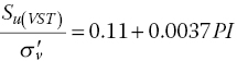
where Su(VST) is the undrained shear strength obtained from the vane shear test and PI is the plasticity index of the clay (expressed as a percentage).
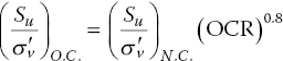
For overconsolidated clays, the Su /σv' ratio has been found to increase with the overconsolidation ratio, OCR, where OCR = (past maximum vertical effective stress)/(in situ vertical effective stress), and the ratio is typically greater than 0.6. The following two equations have been proposed for overconsolidated clays (Ladd et al., 1977):
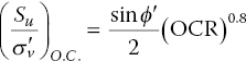
Ladd (1991) suggests using ![]() . Jamiolkowski et al. (1985) suggests the
. Jamiolkowski et al. (1985) suggests the ![]() ratio be taken as 0.23 ± 0.04 for lightly overconsolidated clays of OCR ≤ 2. Mesri (1989) and Terzaghi et al. (1996) recommend that the
ratio be taken as 0.23 ± 0.04 for lightly overconsolidated clays of OCR ≤ 2. Mesri (1989) and Terzaghi et al. (1996) recommend that the ![]() ratio be set as 0.22 for stability analysis involving inorganic soft clays and silts. For organic soils, excluding peats, an
ratio be set as 0.22 for stability analysis involving inorganic soft clays and silts. For organic soils, excluding peats, an ![]() ratio of 0.26 has been recommended by Terzaghi et al. (1996).
ratio of 0.26 has been recommended by Terzaghi et al. (1996).
The empirical correlations for the ![]() ratio as noted above can be used for preliminary estimate of undrained shear strength Su as a function of depth for a clay deposit. Example 1.7 illustrates how to estimate the undrained shear strength as a function of depth for a clay stratum where the OCR can be estimated. It is important to bear in mind that the value of the undrained shear strength of a clay obtained by different test methods may vary significantly (Mayne, 2006). For example,
ratio as noted above can be used for preliminary estimate of undrained shear strength Su as a function of depth for a clay deposit. Example 1.7 illustrates how to estimate the undrained shear strength as a function of depth for a clay stratum where the OCR can be estimated. It is important to bear in mind that the value of the undrained shear strength of a clay obtained by different test methods may vary significantly (Mayne, 2006). For example, ![]() ratio of 0.14 as determined by unconfined compression tests, 0.275 by UU triaxial tests, 0.21 by field vane shear tests, and 0.34 by plane‐strain tests have been reported for Boston Blue clay. Use of the empirical correlations must be made judiciously.
ratio of 0.14 as determined by unconfined compression tests, 0.275 by UU triaxial tests, 0.21 by field vane shear tests, and 0.34 by plane‐strain tests have been reported for Boston Blue clay. Use of the empirical correlations must be made judiciously.
Some clays are quite sensitive to remolding and can lose considerable strength due to disturbance. The ratio of undrained shear strengths in an undisturbed state and in a remolded state (at the same water content) is called sensitivity. Sensitivity for most clays is between 2 and 4, and could be as high as 16 or even higher for highly sensitive clays. Possible loss of strength of sensitive clays due to disturbance (e.g., pile driving during construction) should be accounted for in design.
As noted at the beginning of Section 1.5.2, the undrained condition is not always the most critical condition for designs involving clays. There are situations in which shear strength tends to decrease with time. Obviously, short‐term undrained shear strength will no longer correspond to the most critical condition in these cases. Duncan and Wright (2005) have given a comprehensive list of causes where resisting shear strength increases with time and where shear stress increases with time. Three cases related closely to earth walls where shear strength of clay would reduce with time are as follows:
- Excavation in clay: Upon excavation in clay, the overburden above the new ground surface is removed. The clay underneath the new surface will have a tendency to swell and loses its shear strength with time.
- Rise of free water level in a clay stratum: As a result of a rise of free water level (usually as a result of snow melt or prolong heavy rainfall), the effective stress in the zone where rise of ground water occurred will reduce from moist unit weight to submerged unit weight, hence there will be a gradual decrease in shear strength with time. Rise of free water level usually occurs very slowly in clay. However, this is not the case with a stiff clay stratum where fissures are often present. Water can percolate into the fissures in stiff clays and gradually soften the clay and reduce shear strength with time.
- Non‐durable geo‐materials: Clay shale and clay stones have sometimes been broken up and used as fill material or foundation material for earth walls. The material can be compacted into seemingly stable fill. Over time, however, if wetted by ground water, the fill material will soften and the shear strength will reduce considerably.
We shall examine more closely the case of excavation in clay which is involved occasionally in construction of earth walls. Let us consider an excavation in a moderately overconsolidated clay where the excavation is being carried out fairly rapidly at an approximately uniform rate, and that no drainage of the clay occurs during excavation. Figure 1.33(a) shows the configuration of excavation and the free water levels (FWL) before and after excavation. Figure 1.33(b) shows the change in height of the soil above point P and the change in shear stress on a potential slip plane passing through point P. The shear stress is seen to increase linearly with time during excavation and becomes a constant thereafter. Figure 1.33(c) shows the porewater pressure at point P. It is seen that the initial and final values of porewater pressure are dictated by the original and final free water levels. Between the two, as a result of reduced load, the soil will swell and cause a reduction in porewater pressure during excavation, then try to reacquire equilibrium. Since there is little drainage during excavation, the shear strength will remain essentially constant. After excavation is completed, however, the strength will decrease with time because of swelling of the clay due to load reduction, as shown in Figure 1.33(d). Two observations can be made: (i) during excavation, the shear stress increases with time while the shear strength remains constant, and (ii) after excavation is completed, even though the shear stress is constant, the shear strength reduces with time, hence there is a continued decrease in the factor of safety, as seen in Figure 1.33(e). For a cut in clay, the factor of safety will be a minimum after the porewater pressure has increased to the hydrostatic value, which will occur long after excavation has been completed. Hence, use of the undrained shearing resistance before excavation to evaluate the stability of a cut slope would be unsafe. It is therefore necessary to use long‐term strength, i.e., effective strength parameters, for stability analysis.
Figure 1.33 Changes in porewater pressure and factor of safety during and after a cut is made in a moderately overconsolidated clay (modified after Bishop and Bjerrum, 1960)
For the purposes of comparison, similar plots for an embankment constructed over a saturated moderately overconsolidated clay foundation are shown in Figure 1.34. In this case, the soil will begin consolidation right after the embankment construction is completed. The porewater pressure will dissipate with time and lead to increasing shear strength with time. As a result, the most critical condition is at the end of embankment construction. Because the shearing resistance of the soil is approximately constant during construction, we can assume the shear strength at the end of construction is the same as that before construction. Therefore, the undrained shear strength of the clay foundation should be used for stability analysis.
Figure 1.34 Change in porewater pressure and factor of safety during and after construction of an embankment over a saturated moderately overconsolidated clay foundation (modified after Bishop and Bjerrum, 1960)
In the cases where drained shear strength should be used in design (such as the three cases described above), the drained strength of saturated clays can be determined either by conducting CU triaxial tests with porewater pressure measurement or by conducting CD triaxial tests. The value of c′ is zero for normally consolidated clays and greater than zero for overconsolidated clays (see Figure 1.35). The value of c′ of overconsolidated clays increases with the degree of overconsolidation and is usually less than 600 lb/ft2 (29 kPa), whereas the value of ϕ′ generally falls between 20° and 35°, with higher values being associated with lower plasticity index. Example 1.8 illustrates how to determine the strength parameters for the stability analysis of a cut slope.
Figure 1.35 Effective strength envelopes for normally consolidated and overconsolidated clays (modified after Duncan and Wright, 2005)
As noted earlier in this section, stiff clays are generally fissured. The spacing of fissures may vary from 5 mm near the ground surface to more than 50 mm at depth 30 m below the ground surface (Terzaghi et al., 1996). The orientation of the fissures is generally random. These fissures form localized weak planes in a stiff clay. When a small‐size test specimen is used to determine the shear strength of a stiff clay, very different strength values are often obtained from different test specimens. For a test specimen that contains no fissure (such as sample A in Figure 1.36), the undrained shear strength will likely be quite high (say, 3,000 lb/ft2 or 140 kPa); on the other hand, for a test specimen containing fissures (such as sample B in Figure 1.36), the undrained strength will likely be very low (say, 150 lb/ft2 or 7 kPa). When determining the undrained shear strength of a stiff clay, large‐size specimens should be tested so that the strength values will represent the global strength of the clay. When it is difficult to test large‐size specimens, an average value of shear strengths determined from a large number of tests with small‐size specimens may be used as an alternative (remember not to throw away test data that appear odd!).

Figure 1.36 Schematics of two samples taken from an idealized large mass of fissured stiff clay
1.5.3 Shear Strength of Silts
Silts are typically non‐plastic and behave in similar way to very fine sands. However, some silts are plastic and behave like clays. An example of plastic silt is San Francisco Bay mud, which has a liquid limit near 90, a plasticity index of about 45, and is classified as MH per the Unified Soil Classification System. Determination of the shear strength of a silt therefore may follow that of granular soils or that of clays, depending on whether it is non‐plastic or plastic. Also, in terms of particle size and engineering behavior, silts fall between sands and clays. It is often difficult to anticipate whether a silt is better analyzed in a drained condition (as for sands) or an undrained condition (as for clays). When there is doubt over whether a silt should be analyzed drained or undrained, it is best to analyze both conditions to cover the range of possibilities.
For compacted silts, the same laboratory tests used for clays may be used to determine the shear strength of silts. Note that silts are generally moisture sensitive and their compaction characteristics are similar to those of clays. The undrained shear strength of silts has been found to be influenced strongly by water content. Unlike clays, however, reliable correlations are not available for the estimation of the undrained shear strengths of plastic silts. Data for ![]() for different silts have been found to vary widely (Duncan and Wright, 2005).
for different silts have been found to vary widely (Duncan and Wright, 2005).
References
- AASHTO (2014). LRFD Bridge Design Specifications, 7th edition with 2016 interims. American Association of State Highway and Transportation Officials, Washington, D.C.
- Bishop, A.W. and Bjerrum, L. (1960). The Relevance of the Triaxial Test to the Solution of Stability Problems. Proceedings, ASCE Research Conference on the Shear Strength of Cohesive Soils, Boulder, Colorado.
- Bishop, A.W. and Henkel, D.J. (1962). The Measurement of Soil Properties in the Triaxial Test, 2nd edition. Edward Arnold Ltd., London, 228 pp.
- Duncan, J.M. and Wright, S.G. (2005). Soil Strength and Slope Stability. John Wiley and Sons, Hoboken, New Jersey, 297 pp.
- Fung, Y.C. (1977). A First Course in Continuum Mechanics, 2nd edition. Prentice Hall, New Jersey.
- Head, K.H. and Epps, R. (editors) (1982). Manual of Soil Laboratory Testing, Volume II, 3rd edition. Whittles Publishing, Dunbeath, Caithness.
- Holtz, R.D., Kovacs, W.D., and Sheahan, T.C. (2011). An Introduction to Geotechnical Engineering, 2nd edition. Prentice Hall, New Jersey.
- Hunt, R.E. (1986). Geotechnical Engineering Analysis and Evaluation. McGraw‐Hill Book Company, 729 pp.
- Jamiolkowski, M., Ladd, C.C., Germaine, J.T., and Lancellotta, R. (1985). New Developments in Field and Laboratory Testing of Soils. Proceedings, 11th International Conference on Soil Mechanics and Foundation Engineering, San Francisco, Volume 1, pp. 57–153.
- Japanese Foundation Engineering Society (1995). Introduction to Soils and Foundations, Series 21, 330 pp.
- Jewell, R.A. (1996). Soil Reinforcement with Geotextiles. Construction Industry Research and Information Association. CIRIA Special Publication 123, London, 332 pp.
- Kovacs, W.D., Salomone, L.A., and Yokel, F.Y. (1981). Energy Measurements in the Standard Penetration Test. Building Science Series 135, National Bureau of Standards, Washington, D.C.
- Kulhawy, F.H. and Mayne, P.W. (1990). Manual on Estimating Soil Properties for Foundation Design. Electric Power Research Institute, Palo Alto, California.
- Ladd, C.C. (1991). Stability Evaluation during Staged Construction. Terzaghi Lecture. Journal of Geotechnical Engineering, ASCE, 117(4), 540–615.
- Ladd, C.C., Foott, R., Ishihara, K., Schlosser, F., and Poulos, H.G. (1977). Stress‐deformation and strength characteristics. Proceedings, 9th International Conference on Soil Mechanics and Foundation Engineering, Tokyo, pp. 421–494.
- Lade, P.V. (2005). Overview of Constitutive Models for Soils. ASCE Geotechnical Special Publication No. 139, Calibration of Constitutive Models, GeoFrontiers, Austin, Texas, pp. 1–34.
- Leonards, G.A. (1962). Engineering Properties of Soils. In Foundation Engineering, McGraw‐Hill, New York.
- Mayne, P.W. (2006). In‐Situ Test Calibrations for Evaluating Soil Parameters. Characterization and Engineering Properties of Natural Soils, Singapore Workshop.
- Mayne, P.W. (2007). Cone Penetration Testing. NCHRP Synthesis 368, Transportation Research Board, Washington, D.C.
- Mesri, G. (1989). A Re‐evaluation of Su(mob) = 0.22 σp' Using Laboratory Shear Tests. Canadian Geotechnical Journal, 26(1), 162–164.
- NAVFAC (1986). Design Manual 7.02 Foundations and Earth Structures. Bureau of Yards and Docks, U.S. Navy.
- Peck, R.B., Hanson, W.E., Thornburn, T.H. (1974). Foundation Engineering. John Wiley and Sons, New York, 514 pp.
- Perloff, W.H. and Baron, W. (1976). Soil Mechanics Principles and Applications. John Wiley & Sons, New York, 745 pp.
- Robertson, P.K. and Campanella, R.E. (1983). Interpretation of Cone Penetration Tests, Part II: Clay. Canadian Geotechnical Journal, 20(4), 734–745.
- Sanglerat, G. (1972). The Penetrometer and Soil Exploration: Interpretation of Penetration Diagrams – Theory and Practice. Transportation Research Board, National Academy of Sciences, Washington, D.C., 488 pp.
- Schmertmann, J.H. (1978). Guidelines for Cone Penetration Test Performance and Design. Report No. FHWA‐TS‐78‐209, Federal Highway Administration, Washington, D.C.
- Seed, H.B., Tokimatsu, K. Harder, L.F., and Chung, R.M. (1985). Influence of SPT Procedures in Soil Liquefaction Resistance Evaluations. Journal of Geotechnical Engineering, ASCE, 111(12), 1425–1445.
- Skempton, A.W. (1957). Discussion: Further Data on the c/p Ratio in Normally Consolidated Clays. Proceedings, Institution of Civil Engineers, No. 7, pp. 305–307.
- Skempton, A.W. (1986). Standard Penetration Test Procedures and the Effects in Sands of Overburden Pressure, Relative Density, Particle Size, Aging and Overconsolidation. Geotechnique, 36(3), 425–447.
- Tatsuoka, F., Molenkamp, F., Torii, T., and Hino, T. (1984). Behaviour of Lubrication Layers of Platens in Element Tests. Soils and Foundations, 24(1), 113–128.
- Terzaghi, K. (1923) Erdbaumechanik auf Bodenphysikalischer Grundlage. Franz Deuticke, Liepzig/Vienna.
- Terzaghi, K. and Peck, R.B. (1967). Soil Mechanics in Engineering Practice. John Wiley & Sons, New York, 729 pp.
- Terzaghi, K., Peck, R.B., and Mesri, G. (1996). Soil Mechanics in Engineering Practice, 3rd edition. John Wiley & Sons, New York, 549 pp.