
4
Geosynthetics Reinforcement
The concept of reinforced soil originated at least 6,000 to 7,000 years ago. Natural materials such as reeds, twigs, cotton, jute, straw, wood, etc. were first used as tensile inclusion in soil to construct ziggurats, dwellings, roadways, and even the Great Wall of China (Jones, 1985). A common problem for using natural materials as reinforcement in earthwork construction is with biodegradation of these materials due to microorganisms. With the advent of polymers in the early 20th century, a more stable and durable engineered material became available as tensile inclusion for earthwork construction. When properly formulated, polymers with half‐lives of hundreds of years or more can be stable even under harsh environments.
The term geosynthetics refers to polymeric materials that are manufactured and used to help solve civil engineering problems. As proclaimed by Robert M. Koerner, founder of the Geosynthetic Research Institute, “Geosynthetics are bona fide engineering materials and must be treated as such.”
In this chapter, we shall discuss the engineering behavior and properties of geosynthetics that are relevant to the analysis and design of GRS walls, including (i) load–deformation behavior, (ii) creep and relaxation behavior, (iii) soil–geosynthetic interface behavior, and (iv) hydraulic properties. We shall also discuss the advantages and disadvantages of using geosynthetics as reinforcement.
4.1 Geosynthetics as Reinforcement
The American Society for Testing and Materials (ASTM) D4439 defines geosynthetics as “a planar product manufactured from polymeric material used with soil, rock, earth, or other geotechnical engineering related material as an integral part of a man‐made project, structure, or system.” Since the late 1970s, the applications of geosynthetics in earth structure construction have grown several hundred folds. In 2003, for example, annual global usage of 1,400 million square meters of geosynthetics was reported (Cook, 2003). Today, the global market of geosynthetics is over 5,000 million square meters annually.
Geosynthetics originate from natural gas which reacts to form resin in the form of flakes and mixes with additives into different formations to produce various types of polymeric material known as geosynthetics. Different geosynthetic products have been developed to serve five different functions, including,
- filtration (to allow sufficient fluid flow across the plane of geosynthetics while maintaining the integrity of the soil without appreciable loss of soil particles)
- reinforcement (to improve the stiffness and strength of the soil by forming a soil–geosynthetic composite, or to serve as tiebacks/anchors to stabilize potential failure wedges of an earth structure)
- drainage (to allow sufficient fluid flow to occur within the plane of geosynthetics)
- separation (to set apart dissimilar materials so that the functioning of each material is maintained, e.g., geotextiles used below rail track ballast for separation of subgrade from ballast)
- liquid or soil containment (to contain liquid or soil particles).
To fulfill the various functions noted above, different types of geosynthetics have been manufactured, including
- geotextiles
- geogrids
- geonets
- geomembranes
- geocells
- geosynthetic clay liners
- geocomposites.
The common functions of each type of geosynthetics are summarized in Table 4.1. Detailed descriptions and applications of geosynthetics have been given in many excellent books, notably the books by Koerner (1994, 2005), Van Santvoort (1994), Ingold and Miller (1988), and Holtz et al. (1997).
Table 4.1 Functions of different types of geosynthetics (modified after Koerner, 1994)
| Type of Geosynthetic | Separation | Reinforcement | Filtration | Drainage | Liquid/Soil Grain Containment |
| Geotextiles | √ | √ | √ | √ | √ |
| Geogrids | √ | ||||
| Geonets | √ | ||||
| Geomembranes | √ | ||||
| Geosynthetic clay liners | √ | ||||
| Geocells | √ | √ | |||
| Geocomposites | √ | √ | √ | √ | √ |
There are currently more than 600 geosynthetics products available in North America. Among different types of geosynthetics, geotextiles, geogrids, geocells, and geocomposites have been used as reinforcement in reinforcing applications. A brief description of these four types of geosynthetics is given in this section. Note that the function of reinforcement is sometimes a result of synergistic improvement of system performance. In other words, functions of separation, filtration, drainage, and soil grain containment may work synergistically in conjunction with the reinforcing function to improve the performance of an earth structure. Different functions of geosynthetics often behave in such a manner that the total effect is greater than the sum of the individual effects. The term geosynthetic reinforcement is used in this book interchangeably with geosynthetic inclusion, although the former is more appropriate when the primary function of a geosynthetic is reinforcing, while the latter is more appropriate for situations where the synergistic effect of a geosynthetic is emphasized.
Synthetic polymers used for producing geosynthetics include (in descending order of volume of usage) polypropylene (PP), polyester (PET), polyethylene (PE), polyamide (PA), and polyvinyl chloride (PVC). Generally speaking, polyester (PET) has higher strength and stronger resistance to creep than polypropylene (PP) and polyethylene (PE); and polypropylene (PP) and polyethylene (PE) (both belong to the polyolefins family) have tougher resistance to organic and acid attacks than polyesters.
4.1.1 Geotextiles
Geotextiles, when used independently, are the most versatile among all types of geosynthetics, taking up about 3/4 of the geosynthetics market. As seen in Table 4.1, geotextiles are capable of performing one or more of the five functions of geosynthetics: reinforcement, filtration, drainage, separation, and soil containment (also liquid containment, when impregnated).
Like all other types of geosynthetics, geotextiles are made of synthetic polymers. The polymers, in pellets or granules, are heated and converted into synthetic fibers. Most geotextile fibers are made from polypropylene (about 80%) and polyester (about 15%). Only about 5% of geotextile fibers are manufactured from polyethylene, polyamide (nylon), and polyvinyl chloride (PVC).
Geotextile fibers may take one of three forms, namely, filaments, staple fibers, and slit films:
- Filaments are produced by extruding melted polymers through dies or spinnerets. Since this process is continuous, filaments are often called continuous filaments. After the extrusion, filaments are usually drawn to straighten them.
- Staple fibers are obtained by cutting filaments to shorter lengths, typically 20–100 mm (0.8–4.0 in.) in length.
- Slit films are flat, tape‐like, 10–30 mm (0.4–1.2 in.) wide fibers, produced by slitting an extruded plastic film with blades. After slitting, the tape‐like fibers are often drawn to increase their strengths.
The synthetic geotextile fibers are subsequently made into flexible and generally porous fabrics, called geotextiles, by a few different methods. Depending on the method by which the fibers (or yarns) are converted into fabrics, geotextiles are grouped into:
- woven geotextiles
- nonwoven geotextiles
- knit geotextiles
Woven Geotextiles
Woven geotextiles comprise two sets of parallel yarns in two directions (referred to as warp and weft directions, or machine and cross‐machine directions, respectively) by interlacing the yarns in a systematic manner. The two sets of yarns are typically weaved in perpendicular directions. Woven geotextiles are manufactured with one or a combination of the following types of yarns:
- monofilament yarn, made of a single filament
- multifilament yarn, made of fine multiple filaments aligned together
- slit film (or tape) yarn, made of a single slit film fiber
- spun yarn, made of staple fibers interlaced and twisted together to form a single yarn
- fibrillated yarn, made of strands of tape‐like fibers partially attached to one another.
Some examples of woven geotextiles made of different types of yarns are shown in Figure 4.1. Monofilament yarns are often made from polyethylene (PE), multifilament yarns from polyester (PET), and slit film yarns from polypropylene (PP). This allows an informed guess of the polymer type in a woven geotextile.
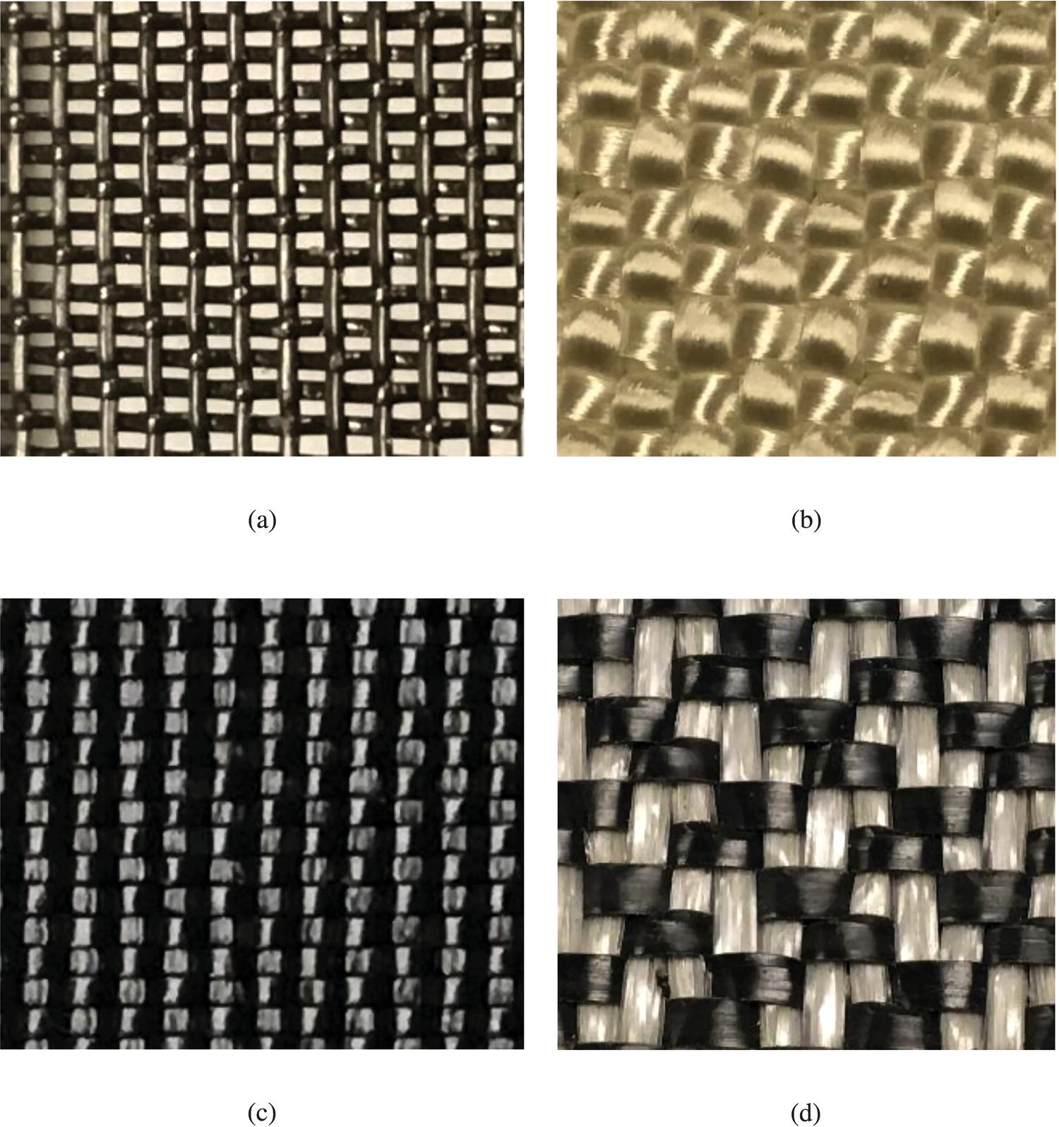
Figure 4.1 Woven geotextiles of different types of yarns: (a) monofilament yarn on monofilament yarn, (b) multifilament yarn on multifilament yarn, (c) slit film yarn on slit film yarn, and (d) multifilament yarn on slit film yarn
Nonwoven Geotextiles
Nonwoven geotextiles are formed by bonding fibers together in an oriented or random pattern. Due to the difference in bonding process, a nonwoven geotextile may be of one of three types:
- needle‐punched (mechanical bonding), see Figure 4.2(a)
- heat‐bonded (thermal bonding), see Figure 4.2(b)
- resin‐bonded (chemical bonding), see Figure 4.2(c).

Figure 4.2 Types of nonwoven geotextiles: (a) needle‐punched, (b) heat‐bonded, and (c) resin‐bonded (side view, courtesy of Fiber Bond)
Needle‐punched geotextiles are formed by punching and withdrawing a bank of thousands of small barbed needles to entangle the fibers of a fibrous web (see Figure 4.3); thermal boned geotextiles are formed by heating and adhering partially melted fibers at crossover points; whereas chemically bonded geotextiles are formed by adding cementing agents (such as acrylic resin) to join the fibers together.
Figure 4.3 Diagram of manufacturing needle‐punched geotextile (INDA, after Koerner, 1994)
Needle‐punched geotextiles, the most common type of nonwoven geotextile, vary widely in weight (100–550 g/m2 or 3–16 oz/yd2) and thickness (varies with normal compressive pressure). Needle‐punched geotextiles have seen applications in filtration, drainage, separation, protection, and as pavement overlay fabrics. Heat‐bonded geotextiles are usually much thinner and denser than needle‐punched geotextiles; hence have higher stiffness at small strains, but with lower drainage capability than needled geotextiles. Resin‐bonded geotextiles are usually much thicker (typically 10–25 mm or 0.4–1.0 in.), stiffer, more expensive, more permeable, and more compressible than other nonwoven geotextiles. Resin‐bonded geotextiles have seen limited applications as liners of golf course bunkers (sand‐traps), as they can provide high permeability and good long‐term durability in a moist and abrasive environment even under low surcharge (Mills, 2005).
Knitted Geotextiles
Knitted geotextiles are formed by knitting loops of one or more nonwoven yarns (other than slit film yarn) to form a planar fabric. Knitted geotextiles are usually of very low stiffness, and have seen limited applications as filters in pipe wrap applications.
4.1.2 Geogrids
Geogrids are plastics formed into an open, grid‐like configuration. The apertures (i.e., openings between the adjacent sets of longitudinal and transverse ribs) of geogrids are large enough, typically between 10 and 100 mm (0.4 and 4.0 in.), to allow soil particles to strike‐through from one side of a geogrid to the other. Because of the large apertures, geogrids have been used almost exclusively for reinforcement applications.
Two major types of geogrids are available. One type is flexible geogrids, or overlapping geogrids. They are textile‐like and formed by overlapping perpendicular polymer strands using a weaving or knitting process, bonding the strands at their junctions, then encasing them with a polymer‐based plasticized coating. Flexible geogrids may be of woven or knitted geogrids, depending on the process by which they are formed. The other type is stiff geogrids, or punched‐and‐drawn geogrids. They are manufactured by drawing a perforated polymer sheet.
Most flexible geogrids are made from PVC‐coated or polypropylene‐coated polyester, while most stiff geogrids are made from high density polyethylene (HDPE) or polypropylene. Flexible geogrids are made about the same strength in both directions or stronger in one direction, as shown in Figure 4.4. Rigid geogrids are available in three forms: uniaxial (stronger in the drawn direction), biaxial (about the same strength in the two drawn directions), or triaxial (with isosceles triangular apertures, about the same strength in the three directions), as shown in Figure 4.5. For cost considerations, uniaxial geogrids are more widely used than other geogrids in reinforced soil walls.
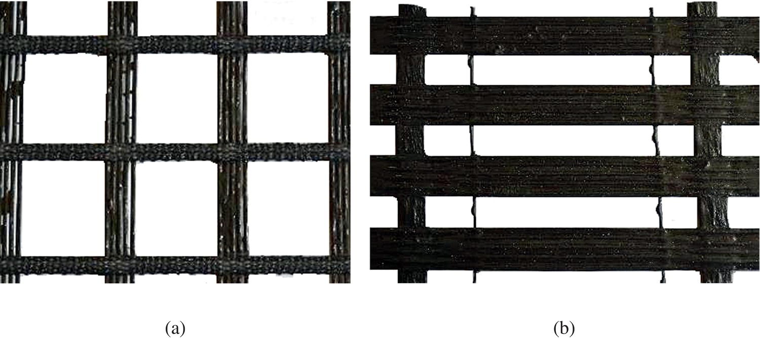
Figure 4.4 Flexible geogrids: (a) uniaxial geogrid and (b) biaxial geogrid
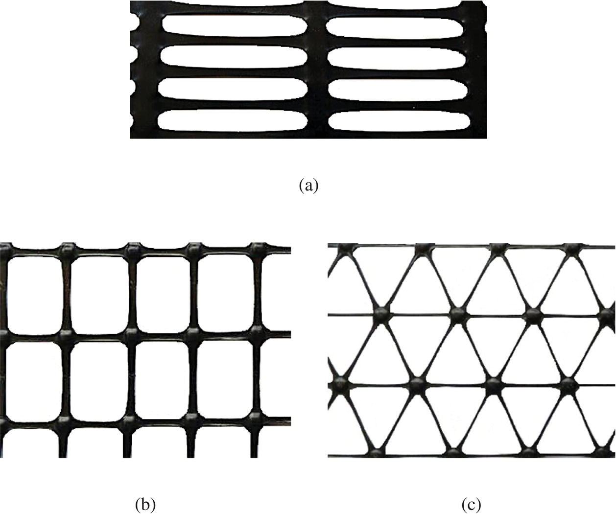
Figure 4.5 Rigid geogrids: (a) uniaxial geogrid, (b) biaxial geogrid, and (c) triaxial geogrid
4.1.3 Geocells
Geocells, as shown in Figure 4.6(a), are a three‐dimensional geosynthetic honeycombed cellular confinement system developed primarily for slope protection or earth retention applications. Geocells are typically formed by extruding from polymeric materials into strips welded together ultrasonically in series. In field installation, the strips are expanded in the opposite direction to form the side‐walls of cells (which is often textured or perforated) to accommodate soil. Fill is placed inside the cells in an expanded state and is compacted after placement. The cellular confinement is said to reduce the lateral movement of soil particles and form a stiffened mat that can distribute vertical loads over a wider area.
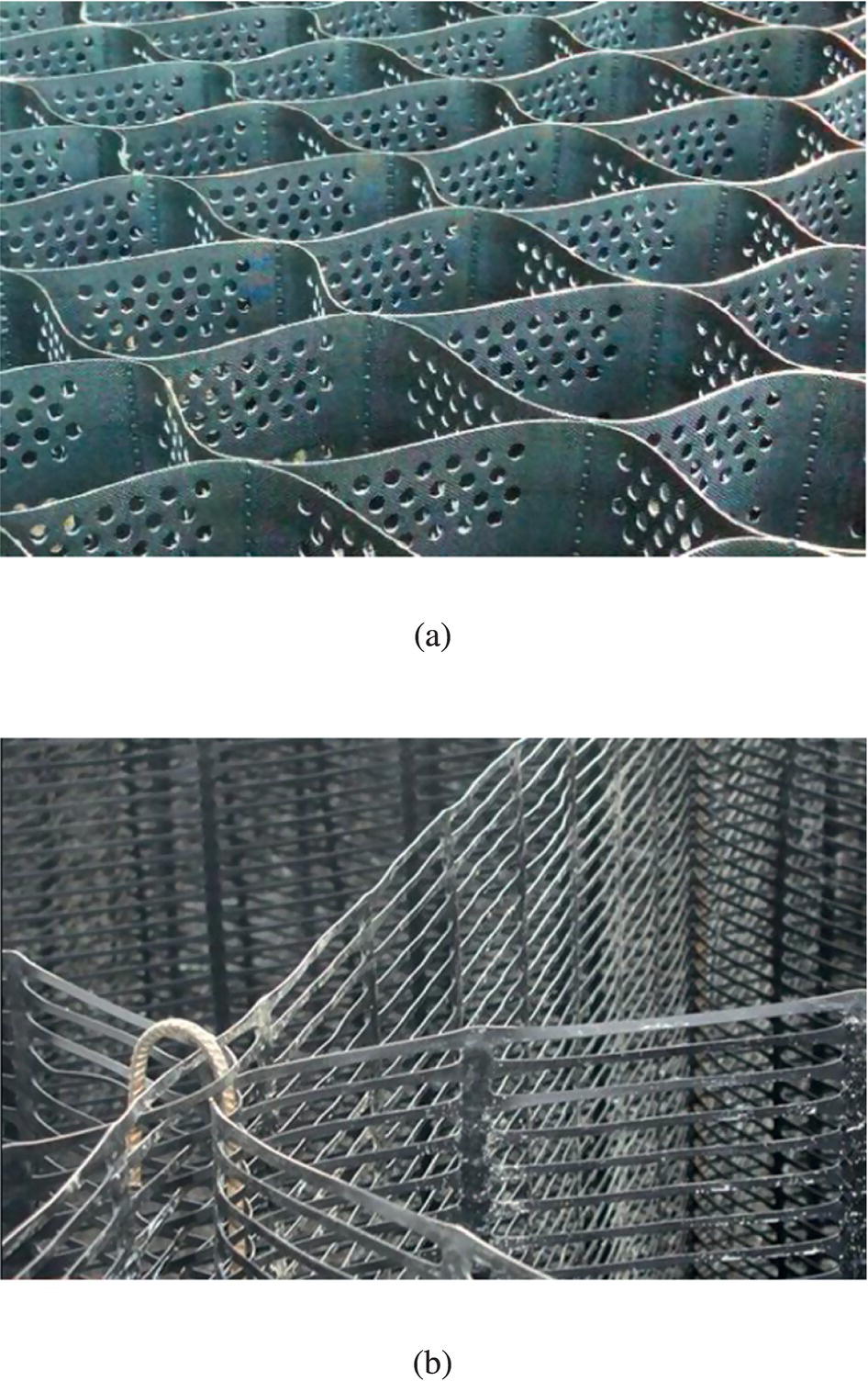
Figure 4.6 Geocells: (a) a geocell made with ultrasonically‐welded high‐density polyethylene (HDPE) (courtesy of Strata Systems, Inc.) and (b) a geocell mattress secured at intersections by metallic bodkins
There is a thicker version of geocells (up to 1 m or 3 ft thick, typical), known as a geogrid mattress or geocell mattress. A geogrid/geocell mattress is a continuous cellular mat fabricated on site by securing vertically positioned geogrids at their intersection with polymer rods or metallic bodkins (see Figure 4.6(b)).
As opposed to planar geosynthetic reinforcement (in the form of sheets) of which lateral confinement is induced by soil–reinforcement interface friction, geocells use their sidewalls to provide lateral confinement. For fill materials that cannot develop sufficiently high interface friction with other fill particles (hence are difficult to compact) or with geosynthetic sheets, geocells may prove to be better reinforcing geosynthetics. An example of such a fill material is uniform‐size (i.e., poorly graded) aggregates.
4.1.4 Geocomposites
As noted earlier in Section 4.1, a number of different types of geosynthetic products have been manufactured to fulfill different individual functions, with each type of geosynthetic product having some distinct advantages over others in a given application. Geocomposites are formed by combining two or more types of geosynthetic products in the manufacturing process to obtain the combined advantages of the different geosynthetic products. A long array of geocomposites is now available (see Figure 4.7(a)). For instance, a needled geotextile/geogrid composite combines the drainage function of a needle‐punched geotextile (when deployed in low permeability backfill) and the reinforcing function of a geogrid. Geocomposite drains can be prefabricated strip drains formed by encasing a nonwoven geotextile (functioning as a filter) over a fluted or dimpled polymeric unit (functioning as a conduit for fluid flow), as shown in Figure 4.7(b). Geocomposite drains can also be drainage mats formed by sandwiching a polymeric drain unit between nonwoven geotextiles, as shown in Figure 4.7(c). Geocomposite drains have been installed along excavation limits (behind the retained earth zone) to minimize subsurface water entering the reinforced zone of reinforced soil walls.
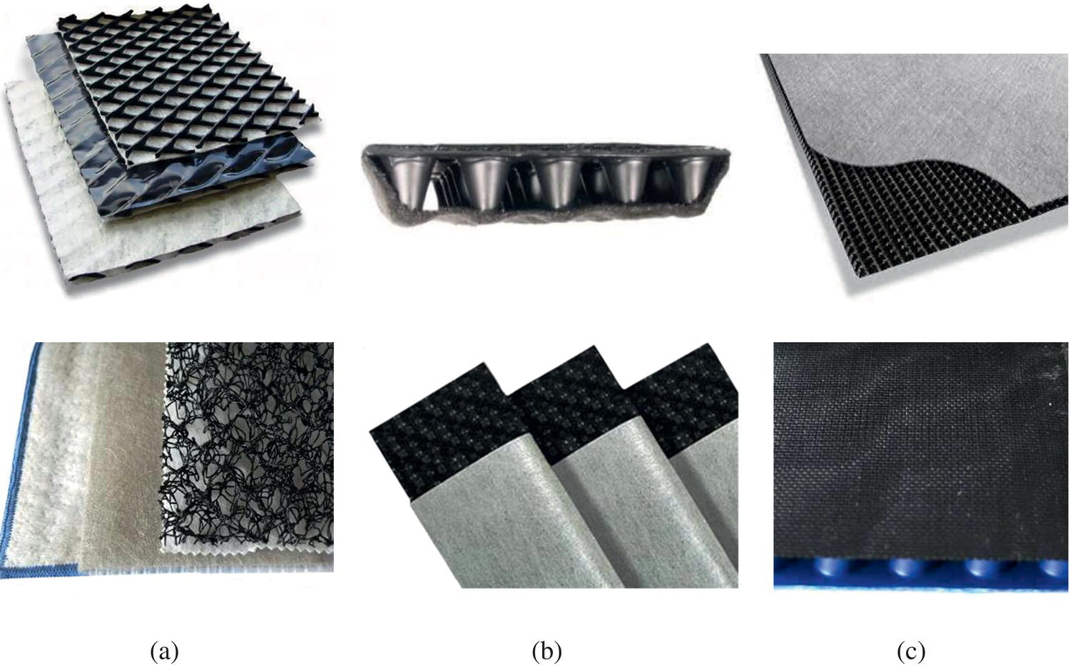
Figure 4.7 Examples of (a) geocomposite, (b) geocomposite strip drain, and (c) geocomposite mat drain
For obvious reasons, there has been considerable advancement and innovation of geocomposites in recent years. This trend will likely continue for many years to come as new applications of geosynthetics are realized, and new and improved geosynthetics products are developed.
4.1.5 Description of Geosynthetics
It has been suggested that the description of a geosynthetic be given by following a certain order (Holtz et al., 1997):
- polymer type (polypropylene, polyester, high density polyethylene, etc.)
- fiber/yarn type, if applicable (monofilament, multifilament, slit film, etc.)
- manufacturing process, if applicable (woven, nonwoven, needle‐punched, etc.)
- primary type of geosynthetic (geotextile, geogrid, geocomposite, etc.)
- mass per unit area and/or thickness, when appropriate
- additional information related to specific applications.
Examples: a polyester multifilament woven geotextile, 240 g/m2 (7 oz/yd2); a polypropylene staple filament needle‐punched nonwoven geotextile, 350 g/m2 (10.5 oz/yd2); a polyethylene extruded biaxial geogrid, with 25 mm × 25 mm (1.0 in. × 1.0 in.) openings.
4.1.6 Costs
The costs of geotextiles, geogrids, and geocomposites depend largely on polymer type, manufacturing process, weight, and locality. In terms of polymer type, the costs in descending order are polyester > polyethylene > polypropylene. In terms of manufacturing process, weaving usually costs more than the nonwoven forming process. Within nonwoven geotextiles, resin‐bonding generally costs more than heat‐bonding, with needle‐punching being the least expensive process.
As of 2018, the costs of nonwoven geotextiles per square meter were typically between $0.15 and $1.5 for light‐weight geotextiles (weight 100–170 g/m2 or 3–5 oz/yd2), between $0.3 and $3 for medium‐weight geotextiles (weight 200–270 g/m2 or 6–8 oz/yd2), and between $0.7 and $4 for heavy‐weight geotextiles (weight 300–550 g/m2 or 9–16 oz/yd2). Woven geotextiles usually cost between $0.25 and $5 per square meter. The cost of geogrids per square meter typically ranges from $0.50 to $2.50, but can be as high as $5 to $8 (Note: 1 m2 ≈ 1.2 yd2).
4.2 Mechanical and Hydraulic Properties of Geosynthetics
The mechanical properties of geosynthetics, including tensile stiffness/strength properties, creep properties, soil–geosynthetic interface properties, tear strength, puncture strength, fatigue strength, and seam strength, have been addressed in a number of books on geosynthetics (e.g., Koerner, 1994, 2005; Van Santvoort, 1994; Holtz et al., 1997), and hundreds of journal articles. In this section, we shall discuss the first three aforementioned mechanical properties as related to the analysis and design of GRS structures. Hydraulic properties related to GRS are briefly discussed at the end of this section.
4.2.1 Load–Deformation Properties of Geosynthetics
The constitutive behavior of civil engineering materials is typically expressed in terms of stress versus strain relationships. The constitutive relationships of geosynthetics are commonly expressed in terms of load/width versus deformation (Note: The term deformation can be regarded as being interchangeable with strain). The main reason that load/width is used, as opposed to stress (load/area), is because the thickness of some geosynthetics is pressure‐dependent. It is important to note that the slope of the load/width versus strain curve is not Young’s modulus (E), rather it is the product of Young’s modulus (E) and thickness (t). The product of E · t has been used to denote the tensile stiffness of a geosynthetic product.
The load–deformation behavior of geosynthetics, commonly characterized by the behavior a uniaxial loading condition, can be divided into two groups: behavior in an unconfined condition (also referred to as in‐air or in‐isolation behavior) and behavior in a confined condition. The former refers to a condition where a geosynthetic specimen is tested in isolation, while the latter refers to a condition where a geosynthetic specimen is tested under pressure or soil confinement to better simulate the operative condition of a geosynthetic product.
(A) Unconfined Load–Deformation Tests
A number of different types of unconfined load–deformation test device with different specimen sizes, clamping methods, and clamp sizes have been developed to measure the in‐air or in‐isolation load–deformation behavior of geotextiles and geogrids. Figure 4.8 shows schematic diagrams of four test methods for measuring the load–deformation and strength properties of geosynthetic products in an unconfined condition, including (i) the grab tensile test (ASTM D4632 for geotextiles), (ii) the wide‐width tensile test (ASTM D4595 for geotextiles, with ASTM D6637 as a parallel test for geogrids), (iii) the plane‐strain test, and (iv) the biaxial test. The results of the first two test methods have routinely been reported by geosynthetics manufacturers and used in design (especially the wide‐width tensile test) and specifications. The plane‐strain test and the biaxial test, although arguably give better simulation of the typical loading conditions of geosynthetics in reinforced soil structures, are not as widely available; their use has been limited to research purposes.
Figure 4.8 Test methods for measuring the load–deformation relationship or strength of geotextiles: (a) grab tensile test, (b) wide‐width tensile test, (c) plane‐strain tensile test, and (d) biaxial tensile test (modified after Myles, 1987)
The grab tensile test for geotextiles (ASTM D4632), Figure 4.8(a), uses a test specimen of B = 100 mm (4.0 in.), L = 150 mm (6.0 in.), and W = 25 mm (1.0 in.) gripped by a pair of jaws along the centerline at opposing ends. The value of the grab tensile strength has been reported by the manufacturer for many geotextiles. For GRS walls, however, grab tensile strength can only be used as an index property, and could be used only as a reference for establishing comparative strengths of different geotextiles.
The wide‐width tensile test for geotextiles (ASTM D4595), see Figure 4.8(b), uses a geotextile specimen of B = 200 mm (8.0 in.) and L = 100 mm (4.0 in.). The specimen is loaded uniaxially at a constant strain rate of 10 ± 3% per minute, under a temperature of 21 ± 2°C, and by a pair of fixed clamps or wedge clamps. Unlike the grab tensile tests, the grips of wide‐width tensile tests extend over the entire width of the test specimen. Wide‐width ultimate tensile strength and stiffness at 5% strains have been commonly reported by the manufacturers of geotextiles that are intended for reinforcing applications. The value of the wide‐width strength (and sometimes 5% stiffness as well) has often been used in design and analysis of GRS and GMSE walls.
Serrated wedges such as the one shown in Figure 4.9(a) have been used to grip geotextiles in wide‐width tensile tests of geotextiles. For higher strength geotextiles (say, strength greater than about 50 kN/m), slippage or damage may occur in the grip area of the test specimen before ultimate strength is reached, therefore roller grips (in combination with extensometers), see Figure 4.9(b), or special clamps may be needed. One special clamping method that has had good success is to treat the grip area of the geotextile specimen with a high‐strength epoxy, and, if needed, reinforce the grip area with metal plates to prevent deformation of the specimen in the gripping area (Ling et al., 1992; Wu and Su, 1987), as shown in Figure 4.9(c).

Figure 4.9 Methods to grip test specimens for load–deformation testing of geotextiles: (a) serrated wedge grips, (b) roller grips, and (c) rigid grips
For measuring the tensile properties of geogrids, test methods for single rib and multiple ribs (ASTM D6637) have been used. To perform a multiple ribs test, the width of the geogrid specimen needs to be at least 200 mm (8 in.) and contain a minimum of five ribs in the cross‐direction. At the start of a test, the distance between the clamps or the distance from centerline to centerline of the rollers should be adjusted to the greater distance of three junctions or 200 ± 3 mm (8.0 ± 0.1 in.), such that at least one transverse rib is contained centrally within the gauge length. Also, at least one clamp must be supported by a free swivel or universal joint to allow the clamp to rotate in the plane of the geogrid specimen. The test method also recommends a strain rate of 10 ± 3% per minute.
It should be noted that with a specimen aspect ratio (width/gauge length) of 2, as stipulated in the wide‐width tensile test for geotextiles (ASTM D 4595), a significant Poisson effect (also known as necking) can occur for most nonwoven geotextiles and geogrids. The Poisson effect is negligible for woven geotextiles of which the deformation of transverse yarns is hardly affected by the deformation of longitudinal yarns (Wu and Tatsuoka, 1992). The Poisson effect generally results in a weaker load–extension response. Figure 4.10 shows the influence of the specimen aspect ratio on the load–deformation relationships of a nonwoven geotextile. It is interesting that the figure also includes the load–deformation curve of a specimen with an infinite aspect ratio, achieved by sewing the geosynthetic specimen into a cylindrical shape end‐to‐end, as shown in Figure 4.11.
Figure 4.10 Influence of specimen aspect ratio on the load–deformation relationship of a nonwoven geotextile in an unconfined condition (modified after Yamauchi, 1987)
Figure 4.11 Setup of a geosynthetic specimen of an infinite aspect ratio in the uniaxial load–deformation testing of geotextiles (modified after Yamauchi, 1987)
The plane‐strain tensile test shown in Figure 4.8(c) is designed to minimize the Poisson effect in a test specimen. To obtain a more accurate load–deformation relationship of woven geotextiles and geogrids that are deployed in a continuous manner in field installation (as opposed to overlapping one sheet over the other), a larger aspect ratio (say, no less than 6) has been recommended for geosynthetic products sensitive to the specimen aspect ratio (Ling et al., 1992), i.e. for most nonwoven geotextiles and geogrids.
The load–deformation curves of geosynthetics can vary significantly depending on polymer type and manufacturing method. Representative uniaxial load–deformation curves are depicted in Figure 4.12. The curves shown in this figure are for general references only; actual curves may vary considerably.
Figure 4.12 Uniaxial load–deformation relationships for different representative geosynthetics of comparable unit weights
The load–deformation behavior of geosynthetics measured in the laboratory is also affected by the rate of extension (i.e., strain rate) and temperature. Generally speaking, the tensile stiffness and strength of geosynthetics tend to increase with increasing strain rate. This may be an important factor to consider in design. The strain rates in actual field installation are typically much smaller than those used in laboratory testing. The effect, however, is different for different polymer types (Van Santvoort, 1994). The influence of strain rate is usually rather significant for polyethylene geosynthetics (e.g., see Figure 4.13(a)) and negligible for polyester geosynthetics, unless the strain is very large (greater than about 7–9% strain for the polyester geotextile shown in Figure 4.13(b)).
Figure 4.13 Illustrative uniaxial load–deformation relationships of (a) a polyethylene geotextile and (b) a polyester geotextile, as influenced by strain rate
Temperature is also known to affect the tensile stiffness and strength of geosynthetics. Tensile stiffness and strength of geosynthetics tends to increase with decreasing temperature (e.g., see Figure 4.14). The load–deformation properties of geosynthetics have typically been reported at an ambient temperature of 21 ± 1°C (70 ± 2°F). In situations where geosynthetic reinforcement is expected to be in an environment where in‐ground temperatures may go well above 21°C (70°F), substantial reduction in strength and stiffness should be used in the design. On the other hand, in situations where the in‐ground temperatures may be much below 21°C (70°F), the geosynthetic reinforcement will likely be less ductile, i.e. having a lower elongation to break (Bonaparte et al., 1987). For most applications in the U.S., the in‐ground temperature is typically lower than 21°C (70°F), hence reported load–deformation properties at 21 ± 1°C (70 ± 2°F) in those applications are slightly on the conservative side in terms of stiffness and strength, and unconservative in terms of ductility.
Figure 4.14 Illustrative uniaxial load–deformation relationships of a polyethylene geotextile, as influenced by temperature
(B) Confined Load–Deformation Tests
Since geosynthetics reinforcements are subjected to soil confinement in actual installation, many confined tensile tests have been proposed (e.g., McGown, et al., 1982; Christopher et al., 1986; Siel et al., 1987; Leshchinsky and Field, 1987; Kokkalis and Papacharisis, 1989). A common objective of these confined tensile tests is to determine the load–deformation properties of geosynthetics under typical operative conditions in field applications. Wu (1991) has given an overview of various confined tests and pointed out that confined tests are only needed for pressure‐sensitive geosynthetics (i.e., needled geotextiles). The shortcomings of each confined tests reported in the literature were discussed.
A common flaw with many confined tensile tests for investigating the load–deformation behavior of geosynthetics is that the measured load–deformation behavior inadvertently includes soil–geosynthetic interface friction as part of the resistance to deformation. Take the confined test method shown in Figure 4.15 as an example, as the soil is held “stationary”, in order for the geosynthetic specimen to deform under applied tensile loads, it must also overcome the frictional resistance induced at the soil–geosynthetic interface. Because the soil in a GRS structure will likely deform with the geosynthetic reinforcement until the reinforced soil structure is approaching failure, any test method that includes soil–geosynthetic interface shear resistance for determination of load–deformation behavior is unsafe. In other words, such a confined test will give a poor representation of typical operating conditions and is unsafe. For a confined test to give representative (and conservative) load–deformation behavior, the soil should only provide pressure confinement, not frictional resistance at the interface (Wu, 1991).
Figure 4.15 Schematic of a confined load–deformation test of which the measured loads include soil–geosynthetic interface frictional resistance, i.e., interface slippage is forced to occur
Soil‐confined tests, such as the uniaxial tension test proposed by Ling et al. (1992) and a modified triaxial test proposed by Wu and Arabian (1990), in which tensile loads are applied to a soil‐confined geosynthetic specimen and the confining soil without inducing soil–geosynthetic interface friction, are shown in Figure 4.16. Because the only function of the soil in these tests is to transmit confining pressure, the soil confinement in these tests can be replaced by a flexible membrane to exert pressure confinement (Ling et al., 1992).
Figure 4.16 Schematic of soil‐confined load–deformation tests without including the soil–geosynthetic interface frictional resistance in the measured loads: (a) a uniaxial tension test (Ling et al., 1992) and (b) a modified triaxial test
A confined tensile test that is conducted by enclosing a geosynthetic specimen by flexible membrane and using a vacuum to supply confining pressure (see Figure 4.17) is referred to as an intrinsic confined tensile test. The load–deformation behavior obtained from an intrinsic confined test is essentially the same as that obtained from a confined in‐soil test where soil–geosynthetic interface slippage is not forced to occur (see Figure 4.18). Among geosynthetic products used as reinforcement for reinforced soil walls, needle‐punched geotextiles have been found to be the only type of geosynthetics of which load–deformation behavior is affected appreciably by pressure confinement within the practical range of confining pressure in actual wall installation. For other types of geosynthetics (i.e., woven geotextiles and geogrids), the load–deformation behavior is essentially the same in unconfined and confined conditions. In summary, other than nonwoven needle‐punched geotextiles, an unconfined test should be used for measuring load–deformation behavior. For nonwoven needle‐punched geotextiles, an intrinsic confined test is recommended.
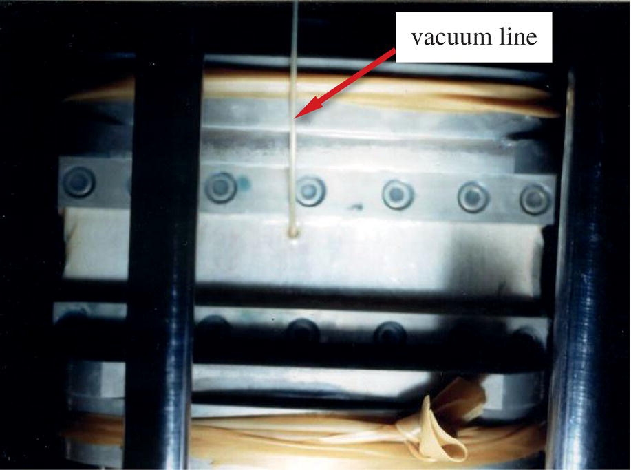
Figure 4.17 Test specimen in the intrinsic confined load–deformation test; the specimen is enclosed by an air‐tight rubber membrane with a vacuum line attached
Figure 4.18 Load–deformation relationships of a nonwoven needle‐punched geotextile under different confinement conditions (Ling et al., 1992)
Uniaxial load–deformation relationships of geosynthetics are generally nonlinear after the strain exceeds a certain value. For design purposes, the load–deformation behavior of a given geosynthetic product can be characterized by an ultimate strength and a stiffness value. The latter can be the secant modulus over the anticipated range of strain, which is the slope of a straight line drawn between the point of largest anticipated strain and the origin, as shown in Figure 4.19. Note that the secant modulus gives the average value of the tangent moduli over the range of strains under consideration.

Figure 4.19 Secant modulus of a load–deformation relationship over an anticipated range of strain
For most woven geotextiles and geogrids in reinforcing applications, a conservative value for the largest strain under service loads can be taken as 1.0–3.0%. Product data published annually by the Industrial Fabrics Association International (IFAI) (known as the Geosynthetics Specifier’s Guide) have reported stiffness at 5% strain and ultimate strength obtained from ASTM D4595 (for geotextiles) and D6637 tests (for geogrids). These values have been referred to in routine designs. The reported stiffness values at 5% strain, although conservative, are too low for more sophisticated analysis. Note again that the slope of the uniaxial load–deformation curve is the product of E (Young’s modulus) and t (thickness) of the geosynthetic product. To carry out a plane‐strain finite element analysis, the area (A) and Young’s modulus (E) of geosynthetic reinforcement are usually required as input parameters. Since the axial stiffness of geosynthetic reinforcement is the product of E and A, as long as the correct product (E · A) is used, the actual values of E or A do not matter in the analysis. If the area (A) is set equal to the nominal thickness (t), the value of Young’s modulus E is then the secant slope of the uniaxial load–deformation curve divided by the nominal thickness (t).
4.2.2 Creep of Geosynthetics and Soil–Geosynthetic Composites
Creep is a term refers to time‐dependent deformation of a material under a constant static stress. Geosynthetics, being manufactured with polymers, are considered creep susceptible. Most civil engineers are comfortable with steel, concrete, and timbers in part because they are generally not creep susceptible. Creep has been a major concern for geosynthetic reinforced soil structures.
Stress level, polymer type, manufacturing method, and temperature are known to affect the creep potential of geosynthetics. Figure 4.20 shows the creep behavior of different polymers at stress levels of 20% and 60%. It is seen that polypropylene (PP) and polyethylene (PE) generally exhibit much higher creep deformation than polyester (PET) and polyamide (PA). For geotextiles that are to be loaded over a long period of time (up to 75–100 years), permissible loads on the order of 40–50% of the ultimate tensile strength have been recommended for polyester and polyamide. For polypropylene and polyethylene, recommended permissible loads have been much lower, on the order of 20–25% of the ultimate strength.
Figure 4.20 Creep behavior of different polymers at two load levels: (a) at 20% of the ultimate level and (b) at 60% of the ultimate level (den Hoedt, 1986)
The allowable tensile load of geosynthetic reinforcement used in the prevailing design guides is typically determined by applying a safety factor and a combination of reduction factors to the limiting strengths of geosynthetics determined by short‐ or long‐term laboratory tests. These tests are conducted by applying uniaxial tensile loads directly to a geosynthetic specimen (in a confined or unconfined condition) without any regard to soil–geosynthetic interaction. It is important to note that conducting uniaxial creep tests for a geosynthetic product in the confinement of soil does not mean the soil–geosynthetic interaction is accounted for.
McGown et al. (1982) developed a fairly sophisticated uniaxial tension test device to measure the creep behavior of geotextiles under soil confinement (see Figure 4.21). They conducted a number of tests on different geotextiles and concluded that soil confinement can influence significantly the creep behavior of some geosynthetics. McGown et al. presented the results of their creep tests in the form of a diagram shown in Figure 4.22. The load–deformation relationship that brings a geosynthetic specimen to a prescribed load level is plotted on the left side of the diagram, with time‐dependent creep deformation behavior shown on the right side of the diagram. The sustained load as well as the strain at the onset of the creep test can be seen clearly from the diagram.
Figure 4.21 Schematic of a uniaxial tension test device for investigating the creep behavior of geotextiles under soil confinement (modified after McGown et al., 1982)
Figure 4.22 A diagram for presenting the creep test results of a geosynthetic specimen
Previous discussions on confined load–deformation tests (see subsection (B) of Section 4.2.1) are equally applicable to confined creep tests. That is, since soil and geosynthetic in the operational condition of GRS walls will likely deform in a compatible manner until failure is approached, confined creep tests that include soil–geosynthetic interface resistance in the measured loads are unconservative (i.e., will significantly underestimate creep potential and creep deformation). Note that the test device shown in Figure 4.21 is conceptually sound for studying the creep behavior of pressure‐sensitive geosynthetics because the confining soil and geosynthetic specimen in this test device will deform in a compatible manner. However, the intrinsic confined test described in subsection (B) of Section 4.2.1 is a much simpler alternative. An intrinsic creep test can be conducted by simply applying stained axial loads to a pressure‐confined test specimen under a prescribed vacuum pressure. It is important to emphasize that the intrinsic test is necessary only for pressure‐sensitive geosynthetic products (i.e., needle‐punched geotextiles). For non‐pressure‐sensitive geosynthetics (such as nonwoven geotextiles and geogrids), an unconfined creep test would be sufficient for investigating the long‐term creep behavior.
Since temperature is known to influence the rate of creep of geosynthetics, creep tests should be conducted over the range of temperatures anticipated under the in‐service condition of the reinforced soil structure. This does, however, require extensive testing at different temperatures over long periods of time. In the absence of such information, time‐shifting techniques may be utilized judiciously to account for the temperature effect. Time shifting is especially needed if the anticipated in‐service temperatures are higher than the ambient temperatures under which the creep data are obtained. If these data are used directly in design computations without temperature correction, creep deformation will be underestimated.
Whether or not creep is a design issue for a geosynthetic reinforced soil structure must be evaluated by considering the deformation characteristics of the reinforced soil mass as a whole, i.e., the soil–geosynthetic interaction must be properly accounted for. It can be misleading to evaluate the long‐term creep potential of a reinforced soil structure based on the results of element creep tests performed on geosynthetic specimens alone, as has (inappropriately) been stipulated by most prevailing design guides. Wu and Helwany (1996) developed a simple plane‐strain long‐term soil–geosynthetic interaction test in which the soil and geosynthetic are allowed to deform in an interactive manner. They reported results for two long‐term creep tests: one with a clay and the other with a sand. For the sand‐backfill test, creep deformation essentially ceased within 100 minutes after initiation of the test; whereas the clay‐backfill test experienced continuing creep deformation over the entire test period (18 days); shear failure occurred in the soil on the 18th day. Element tests on the geosynthetic alone would have underestimated the maximum strain by 250% in the clay‐backfill test, and overestimated the maximum strain by 400% in the sand‐backfill test.
To examine soil–geosynthetic interactive behavior in GRS mass by a laboratory test, a simple device was developed by Ketchart and Wu (2001, 2002) by streamlining the test apparatus used in Wu and Helwany’s study (1996). The simplified test is referred to as the soil–geosynthetic interactive performance (SGIP) test and is shown in Figure 4.23. The procedure of the SGIP test can be described as follows:
Step 1 Treat the interior side walls of a SGIP test bin by applying a thin layer of silicon grease to the side walls and covering them with a sheet of latex membrane to minimize soil–wall friction/adhesion (for side wall lubrication, see Section 1.4.3).
Step 2 Lay a sheet of geosynthetic covering the base of the test bin; place and compact the fill material in lifts inside the cuboidal space formed by the side walls and movable supporting plates until the fill reaches the mid‐height of the test bin.
Step 3 Lay a second sheet of geosynthetic specimen over the surface of fill at the mid‐height; continue with placing and compacting the fill material until it reaches the full height of the test bin.
Step 4 Lay a third sheet of the geosynthetic over the top of the compacted fill; position a loading plate over the third geosynthetic sheet.
Step 5 Apply increasing vertical loads to the top surface of the soil–geosynthetic composite until a prescribed sustained load is reached; release the movable supporting plates and measure vertical and lateral time‐dependent deformation while maintaining a constant sustained load; continue monitoring the deformation over a planned test period.
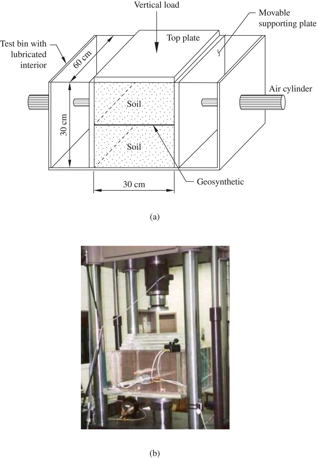
Figure 4.23 The soil–geosynthetic interactive performance (SGIP) test: (a) schematic diagram and (b) a SGIP test loaded by a universal tester (Ketchart and Wu, 2001)
The fill material and geosynthetic specimen used in the test should be the same as those to be used in actual construction, the fill material should be compacted to the anticipated dry density and water content, and the sustained load should correspond to the largest vertical stress anticipated in the reinforced soil structure. The above procedure can only be used for fill material that has sufficient cohesion to allow the test to be conducted in an unconfined condition. For fill material with little or no cohesion, a confining pressure can be applied to the soil–geosynthetic composite by enclosing the entire test specimen in a rubber membrane in an air‐tight condition with vacuum pressure applied.
Ketchart and Wu (2001, 2002) have reported results of SGIP tests on a number of specimens of soil–geosynthetic composites, with a few tests conducted under elevated temperatures to accelerate creep of geosynthetics. A polypropylene nonwoven geotextile, of which the creep rate under 52°C (125°F) has been determined to be between 150 and 250 times faster than that under ambient temperature, was selected for the tests. The fill material was a road base (with 20% of fines, prepared at 95% relative compaction and 2% wet‐of‐optimum moisture) and the soil–geosynthetic composite was subjected to a sustained surcharge of 100 kPa (15 psi) in a 52°C (125°F) environment (see Figure 4.24(a)). Creep deformation of the soil–geotextile composite under the elevated temperature was found to be very small and decreased rapidly with time, as seen in Figure 4.24(b). Creep deformation ceased completely after approximately 12 days, which suggests that creep deformation of the soil–geosynthetic composite would have become negligible after about 6.5 years under ambient temperature. The study concludes that creep of soil–geosynthetic composites is strongly influenced by the creep characteristics of the confining soil. With a well‐compacted granular backfill (such as a road base material), creep of soil–geosynthetic composite is negligible under a sustained surcharge of 100 kPa, much higher than typical design loads of GRS walls in non‐load‐bearing applications.

Figure 4.24 A SGIP test conducted under elevated temperature: (a) test being conducted in a 52°C (125°F) environment inside a temperature incubator and (b) a set of test results (Ketchart and Wu, 2001)
A modified SGIP test was subsequently developed to accommodate larger/taller soil–geosynthetic composite specimens, either for greater reinforcement spacing or for soils of larger grain sizes. The modified SGIP test is shown in Figure 4.25. Note that a confining pressure in the photo is being applied to the soil–geosynthetic composite via a vacuum through a membrane enclosing the entire test specimen (the vacuum is needed for fill materials of little cohesion).
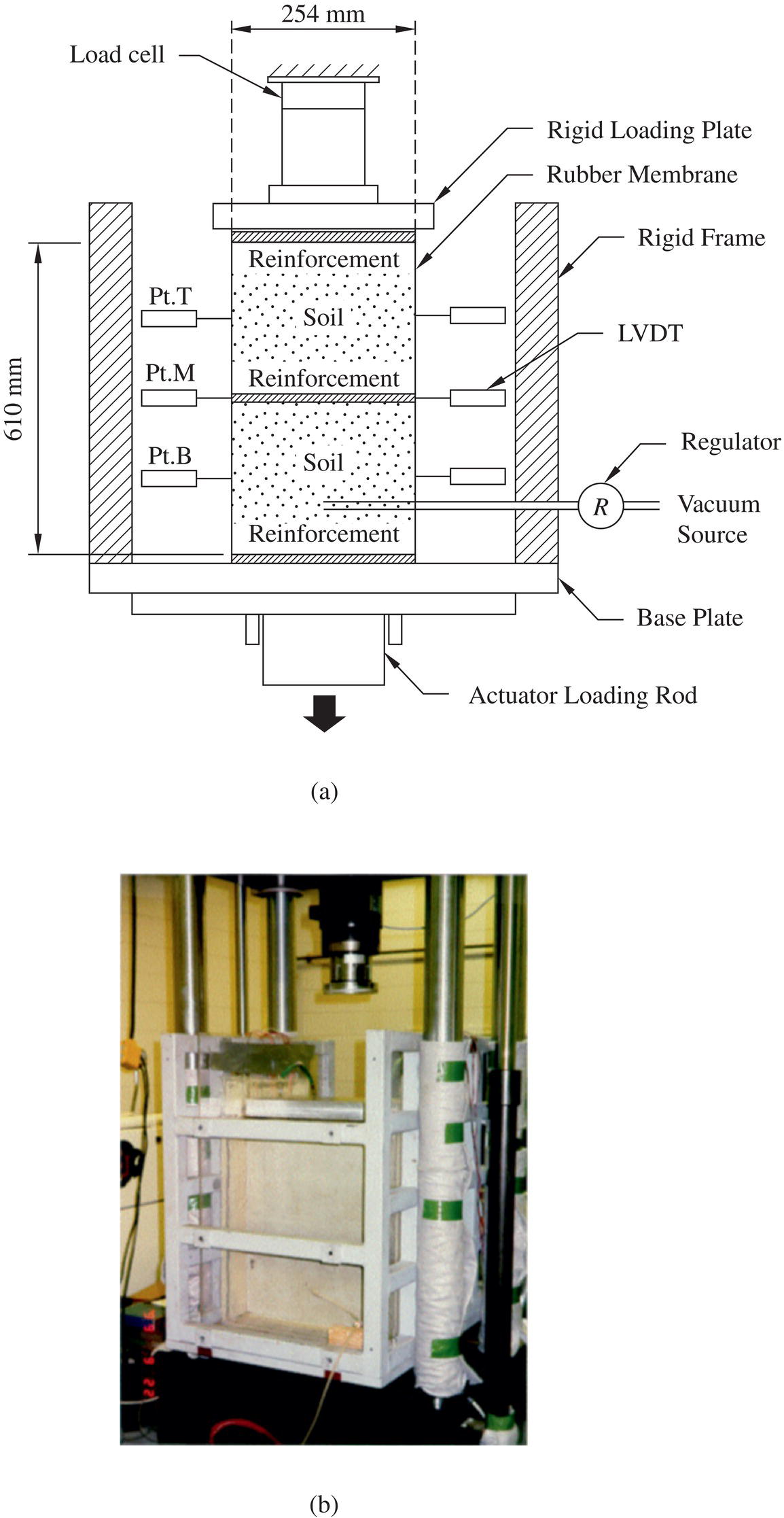
Figure 4.25 A modified SGIP test for taller specimens: (a) schematic diagram of test setup and (b) loaded by a universal tester (modified after Ketchart and Wu, 2001)
There are two unique features in the different generations of the SGIP test. First, a sustained load is applied to the soil, which in turn transfers the loads to the geosynthetic, replicating the typical load transfer mechanism in GRS structures (i.e., loads in geosynthetic reinforcement are transferred from soil through soil–geosynthetic interface bonding to the geosynthetic reinforcement, rather than loads being applied directly to geosynthetic reinforcement as in most creep tests). Second, both the soil and geosynthetic are allowed to deform in an interactive manner under a plane‐strain condition — a very important feature in any properly conducted creep tests of a GRS mass.
Crouse and Wu (2003) summarized the measured behavior of seven full‐scale reinforced soil walls that had been monitored for an extended period of time to examine the long‐term performance. The reinforced soil walls, representing a variety of wall types with granular backfill, including the Glenwood Canyon wall (Bell et al., 1983), the Tanque Verde–Wrightown–Pantano Roads project wall (Berg et al., 1986; Collin et al., 1994), the Norwegian Geotechnical Institute (NGI) project, known as the NGI wall (Fannin and Hermann, 1992), the Japan Railway Test Embankment project, known as the JR wall (Tatsuoka et al., 1992), the Highbury Avenue, the London Ontario project, known as the Highbury wall (Bathurst, 1992), the FHWA Algonquin wall (Simac et al., 1990; Christopher et al., 1994), and the Seattle Preload Fill project, known as the Seattle wall (Allen et al., 1992). The maximum creep strains in the geosynthetic reinforcement were less than 1.5% in all seven walls. Also, the creep strain rate in all these cases decreases with time, and there exists an approximately linear relationship between log (creep rate) and log (time) for all the walls.
Allen and Bathurst (2003) analyzed the long‐term creep data of 10 full‐scale in‐service geosynthetic walls. Post‐construction, long‐term wall face deformation data show that the geosynthetic wall face deformation for the properly designed walls is generally less than 25–30 mm (1.0–1.2 in.) during the first year of service, and less than 35 mm (1.4 in.) over the design lifetime for walls that are lower than 13 m (40 ft) in height. Allen (1991) and Bathurst et al. (1988) also studied geosynthetic reinforcement strains measured in geosynthetic reinforced soil walls and slopes. The maximum strains were found to be on the order of 1–2% or less.
Helwany and Wu (1995) reported some interesting results of finite element analysis on long‐term behavior of two 3.0‐m high geosynthetic reinforced soil walls. The walls were identical in every respect except that one had a clayey backfill and the other a granular backfill. Figure 4.26 shows time‐dependent displacement fields of the two walls. The difference in the displacement fields is evident. In the clay‐backfill wall, the maximum strain in the geosynthetic reinforcement increases by 3.5% from the end of construction to 15 years afterwards. In the granular‐backfill wall, on the other hand, the increase in maximum strain over the same time period is negligible to very small. Note that the very large differences in the displacements and strains occur despite the levels of loads in the two walls being comparable. The analysis suggests clearly that the time‐dependent behavior of the backfill plays a crucial role in the creep deformation of a soil–geosynthetic composite. Similar findings have been reported in studies conducted by Li and Rowe (2008), Skinner and Rowe (2005), Rowe and Taechakumthorn (2008), Bergado and Teerawattanasuk (2008), Liu and Won (2009), Liu et al. (2009), and Li et al. (2011).

Figure 4.26 Time‐dependent displacement fields of two GRS walls: (a) a clayey backfill wall and (b) a granular backfill wall, as obtained from finite element analysis (Helwany and Wu, 1995)
A design protocol for predicting the long‐term creep deformation of a GRS mass has been proposed by Crouse and Wu (2003). The protocol involves conducting a SGIP test by employing the soil and geosynthetic to be used in a design. Because GRS structures with well‐compacted granular soil have been known to have little creep deformation, the protocol is only needed when a “questionable” on‐site soil (in terms of long‐term deformation) is being considered as backfill for a GRS structure or when the load level is unusually high.
4.2.3 Stress Relaxation of Geosynthetics
Stress relaxation is a term used to describe the phenomenon that stress in a material is relieved with progression of time when the material is kept under a constant strain condition. A material which would deform with time under a constant stress is said to be susceptible to creep. Such a material tends to experience stress relaxation if the deformation is held constant. Geosynthetics are known to be susceptible to both creep and stress relaxation. In general, polypropylene and polyethylene are much more susceptible to creep and stress relaxation than polyester. Since deformation of well‐compacted granular soils tends to become quite small soon after load applications and soil–reinforcement tends to deform in a compatible manner (unless when a soil–geosynthetic composite is approaching failure), stress relaxation in geosynthetic reinforcement is a prevalent phenomenon in geosynthetic reinforced soil structures when a well‐compacted granular fill is employed, especially if the geosynthetic reinforcement is polypropylene or polyethylene.
Let us begin the discussion of stress relaxation by reviewing the relationships among stress, strain, and time. Load–deformation–time relationships of polymeric geosynthetics can be expressed in terms of three different sets of planar curves: (i) the isostress curve (commonly referred to as the creep curve), see Figure 4.27(a), (ii) the isochronous curve, see Figure 4.27(b), and (iii) the isostrain curve (also referred to as the relaxation curve), see Figure 4.27(c). For some creep‐susceptible materials, the relationships among time, stress, and strain can be expressed by a curved surface in the stress–strain–time domain. The three curves shown in Figures 4.27(a), (b), and (c) are then the projections of this curved surface onto three perpendicular planes: the isochronous plane, the isostress plane, and the isostrain plane. If a set of projected curves on one of the three planes is known, the projected curves on the other two planes can be obtained as long as the material has a unique stress–strain–time relationship. Limited creep and relaxation tests data have suggested that a unique curved surface exists only for polyester geosynthetics. Example 4.1 illustrates how a set of isostrain (relaxation) curves can be obtained from a set of isostress (creep) curves. This implies that a material susceptible to creep will also be susceptible to stress relaxation.
Figure 4.27 Two‐dimensional representation of load–strain–time relationships: (a) isostress curves (or creep curves), (b) isochronous curves, and (c) isostrain curves (or relaxation curves)
Data obtained from isostrain (relaxation) tests of geosynthetics have revealed that reduction of loads in geosynthetic reinforcement would occur early and rapidly, and decrease with time at a decreasing rate. Kaliakin et al. (2000) have reported results of relaxation tests for 11 geogrids produced by three different manufacturers (see Figure 4.28 for 3 sets of test results). The reductions in loads in the first 100 minutes of the geogrids are seen greater than those in the ensuing month (43,000 minutes).

Figure 4.28 Normalized isostrain curves obtained from stress relaxation tests for different geogrids: (a) a flexible polyester woven geogrid, (b) a rigid HDPE punched‐and‐drawn geogrid, and (c) a rigid polypropylene punched‐and‐drawn geogrid (Kaliakin et al., 2000)
Unlike creep deformation, stress relaxation is not visible. Moreover, because loads in geosynthetics cannot be measured (other than at the extremities), stress relaxation is not as well understood as creep. We can, however, conceptualize stress relaxation of a geosynthetic product by visualizing a simple experiment. Let us picture a creep‐susceptible strip of geosynthetic with one end affixed to the ceiling and the other end attached to a heavy dead weight. Due to the weight, the geosynthetic will experience creep deformation with time. If we are to “stop” the deformation from occurring after the geosynthetic reaches a certain prescribed strain and maintain the strain to be unchanged from that point on, the weight will have to be reduced; to wit, stress relaxation will have to occur. A similar phenomenon will occur when a creep‐susceptible geosynthetic reinforcement is embedded in a well‐compacted granular fill. When the geosynthetic is subject to loads, time‐dependent creep deformation will occur in the geosynthetic reinforcement. Since deformation of the granular fill will cease after a certain time has elapsed, relaxation in the geosynthetic product will then occur after the granular fill ceases to deform. Studies have suggested that relaxation may initiate when the rate of deformation becomes very small, before deformation comes to a completely stop (e.g., Ketchart and Wu, 2001).
Full‐scale experiments of reinforced soil walls have also suggested that significant stress relaxation may occur within a short time after construction provided that well‐compacted granular soil is used in construction. An interesting example is a reinforced soil wall experiment conducted by the Public Works Research Institute (PWRI) of Japan, referred to as the PWRI test wall. The wall was 6.0‐m high with concrete block facing, and the fill was a well‐graded silty sand. The reinforcement was a HDPE polymer grid with a tensile strength of 56.4 KN/m on vertical spacing of 0.5 m. Two different reinforcement lengths were used: 3.8 m (primary) and 1.3 m (secondary). In less than three days after the wall was constructed, the grid reinforcement was cut sequentially at pre‐selected locations as shown in Figure 4.29(a) (Note: The numbers noted on the reinforcement layers indicate the sequence of cutting). Figure 4.29(b) shows the maximum horizontal wall displacement in response to the cutting. It is seen that there was negligible displacement (on the order of 0.1 mm) from Cut No. 1 to Cut No. 50. This suggests that the loads in the geosynthetic reinforcement up to Cut No. 50 have likely reduced to negligible values at the time of cutting. In an attempt to validate the observation in the PWRI test wall, a similar experiment was conducted by Ketchart and Wu on a 3.0‐m high reinforced soil wall built with a compacted well‐graded crushed granular fill and a 70 kN/m woven polypropylene geotextile on 0.3 m spacing (Wu, 2001). The experiment confirmed the observed behavior of the PWRI test wall, in that severing geosynthetic reinforcement within a short time after construction causes negligible deformation (less than 0.1 mm) of the reinforced soil mass.

Figure 4.29 The PWRI test wall: (a) sequence of cutting geosynthetic reinforcement as indicated by numbers above reinforcement layers (cutting stopped at Cut No. 60 when failure occurred) and (b) maximum horizontal wall displacement in response to cutting of geosynthetic reinforcement
In GRS walls, geosynthetic reinforcement is typically subject to the highest load at the end of construction (for non‐load‐bearing applications) or right after placement of heavy loads (in load‐bearing applications, such as girders in bridge abutments). The safety margin against overstress of geosynthetic reinforcement is therefore the lowest at those points in time. Soon after this, stress relaxation will likely occur, and the safety margin with respect to overstress of geosynthetic reinforcement will likely increase with time.
In the literature, loads in geosynthetic reinforcement are sometimes reported, and those loads are typically obtained from (i) load–deformation relationships obtained from the wide‐width tensile test (ASTM D4595 for geotextiles, ASTM D6637 for geogrids) or (ii) isochronouous curves (usually obtained from results of creep tests using a procedure similar to that given in Example 4.1). The former is vastly unreliable as the load–deformation relationship is affected by such factors as strain rate, temperature, specimen aspect ratio, and confinement (see subsection (A) of Section 4.2.1). For the latter, other than polyester geosynthetics, a unique time–stress–strain relationship does not exist. Therefore, reinforcement loads obtained from this approach are deemed unreliable (other than for polyester geosynthetics).
Researchers have developed methods that consider geosynthetics as elasto‐viscoplastic material to determine reinforcement loads (e.g., Peng et al., 2010; Kongkitkul et al., 2010). The viscous property is that of isotach which states that current load in geosynthetic reinforcement is a function of the current strain and the current strain rate, not time. Based on isotach viscosity, creep can be described as a process of increasing strain at decreasing strain rate under a sustained load; load relaxation can be described as a process of decreasing load when the change in the elastic strain (negative) is balanced by the change in the inelastic strain (positive). The approach arguably offers the most rational prediction of reinforcement loads. However, since no method is available to measure loads in geosynthetic reinforcement (other than at the extremities), there has not been direct verification of loads obtained from this approach.
4.2.4 Soil–Geosynthetic Interface Properties
Most design guides of reinforced soil structures require that the tensile reinforcement has sufficient interface bond strength with the fill material. Interface bonding is needed to allow the geosynthetic reinforcement to effectively carry tensile loads and to prevent slippage of reinforcement that may lead to instability.
The interface bond strength between the soil and geosynthetic reinforcement has been evaluated by two test methods: the direct shear interface test and the pullout test, as shown in Figure 4.30. The former applies shear forces to the soil–geosynthetic interface and the latter applies tensile forces to the geosynthetic. In addition to the difference in force application mechanism, the two test methods also differ in geometric configuration, loading/stress path, and boundary conditions. Published data have indicated that interface friction angles determined by the two tests are usually different (Collios et al., 1980; Ingold, 1983; Richards and Scott, 1985; Rowe et al., 1985; Koerner, 1986; Juran et al., 1988). For geosynthetic reinforcement embedded in a dense sand under low overburden pressure, the pullout test tends to give a higher interface bond strength than the direct shear interface test. For geosynthetic reinforcement embedded in loose sand under high overburden pressure, the interface bond strengths obtained from the two tests have been found to be similar. Depending on the application, one of the tests is likely to be more appropriate than the other. For example, the pullout test is more appropriate for evaluating the potential pullout of reinforcement from the anchored zone (see Figure 4.31(a)). The direct shear interface test, on the other hand, is more appropriate for evaluating the slide‐out failure between a soil wedge and the geosynthetic reinforcement beneath it (see Figure 4.31(b)).

Figure 4.30 Test methods for evaluating the interface bond strength between soil and geosynthetic: (a) direct shear interface test and (b) pullout test
Figure 4.31 Conditions for which (a) the pullout test is more appropriate and (b) the direct shear interface test is more appropriate
Direct shear interface tests come in different degrees of constraint on deformation of the geosynthetic specimen and soil–geosynthetic contact area. Figure 4.32 shows three direct shear test devices with different constraints to deformation of the geosynthetic specimen: free geosynthetic, fixed geosynthetic, and fixed geosynthetic with an enlarged base. The test with an enlarged base allows the area of interface shear to remain constant during testing. To perform a fixed geosynthetic direct shear interface test, the geosynthetic (usually geotextiles) is affixed to a wooden block, either by simply covering tightly over the block with clamps at the two ends or affixing the entire surface area of geosynthetic specimen to the block by adhesives. The choice of which type of direct shear interface test to perform should be determined based on the anticipated constraint conditions of the geosynthetic reinforcement in actual applications. The fixed geosynthetic test is usually the test of choice for finite element analysis where the interface element may be simulated as a pair of contacting points. Regardless of the type of direct shear interface test, interpretation of test results for soil–geosynthetic bonding strength is performed by the same procedure as for direct shear tests performed on soils (see Section 1.4.1). The same principles regarding selection of specimen deformation constraint also apply to pullout tests.
Figure 4.32 Three types of direct shear interface tests for evaluation of soil–geosynthetic interface properties with different deformation constraints of geosynthetic specimen: (a) free geosynthetic, (b) fixed geosynthetic, and (c) fixed geosynthetic with an enlarged base
Pullout tests vary widely in the dimensions of test bin, length and width of reinforcement, and constraint on deformation of the geosynthetic specimen. The variations have caused serious confusion, especially with interpretation of test results. The interface pullout formula developed by Sobhi and Wu (1996) is recommended for interpretation of the results measured by pullout tests. The formula was derived based on postulates deduced from findings of large‐scale laboratory pullout tests and finite element analysis. The interface pullout formula is capable of describing with very good accuracy the relationship between tensile force and displacement for any given length of geosynthetic test specimen used in a laboratory pullout test.
The interface pullout formula (Eqn. (4‐1)) gives the relationship between tensile force per unit width (T ) at any given section and the location of the section (denoted by coordinate x) along the length of the test specimen:
where F = applied pullout force per unit width at the load‐application end of test specimen, E = Young’s modulus of geosynthetic reinforcement (obtained from an uniaxial load–deformation test), t = nominal thickness of geosynthetic reinforcement (Note: The product of E and t is the slope of load–deformation curve when the load is expressed as tensile load/width, see Figure 4.19), σn = vertical pressure applied on the planar surface of the geosynthetic specimen, and f = coefficient of friction of the soil–geosynthetic interface.
The interface pullout formula can be used to predict and interpret pullout test results. The following are some example applications, including: (i) to determine the coefficient of friction at the soil–geosynthetic interface, (ii) to predict the applied pullout force needed to bring about complete pullout failure for a given length of geosynthetic specimen, and (iii) to predict displacement at any point for a given applied pullout force at or before pullout failure. Some details for the example applications of the interface pullout formula are given below.
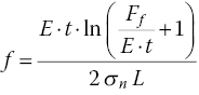
Case A: Use the interface pullout formula to determine the coefficient of friction f at the soil–geosynthetic interface.
Solution: Given the applied force per unit width at failure (Ff) as determined in a pullout test and the total length of the geosynthetic specimen (L), the friction coefficient (f) can be determined by:
Some pullout tests do not reach a failure state when terminated. In which case, if the active length (the length of test specimen over which movement occurred under a given applied pullout force) and the corresponding applied pullout force (prior to failure) are known, these values can be used in lieu of total length (L) and pullout force at failure (Ff) in Eqn. (4‐2).
Case B: Use the interface pullout formula to predict the applied pullout force needed to bring about complete pullout failure for a given length of geosynthetic.
Solution: The applied pullout force F (per unit width) needed to bring about complete pullout failure of a specimen for total geosynthetic length L is:
(4‐3)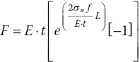
Case C: Use the interface pullout formula to predict the displacement at any point along the length of a geosynthetic specimen when subject to a given pullout force.
Solution: Given a pullout force F (before or at failure), the displacement u at a point along the geosynthetic reinforcement with a coordinate xb can be determined by:
(4‐4)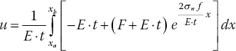
where xa is the coordinate of the active length (the length over which deformation occurred in a pullout test), which can be determined as:
(4‐5)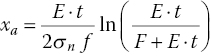
Note that x = 0 corresponds to the section where pullout forces are applied to the geosynthetic specimen.
4.2.5 Hydraulic Properties of Geosynthetics
Filtration and drainage are water flow‐related functions of geosynthetics that may be involved in design and analysis of reinforced soil walls. The term filtration refers to how well a geosynthetic product may retain soil particles as water flows across the plane of geosynthetic product, while the term drainage refers to how easy water may travel within the plane of a geosynthetic product. The cross‐plane permeability is commonly expressed in terms of permittivity (ψ) and in‐plane permeability in terms of transmissivity (θ), which are defined as:
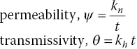
where kn = Darcy’s coefficient of permeability (or hydraulic conductivity) normal to the plane of geosynthetic product
- kh = Darcy’s coefficient of permeability (or hydraulic conductivity) within the plane of geosynthetic product
- t = thickness of geosynthetic product
and the flow rate (q) can be calculated as:
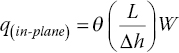
where Δh = loss of total head
- A = total area of geosynthetic product involved in cross‐plane flow
- L = total length of geosynthetic product involved in in‐plane flow
- W = width of geosynthetic product involved in in‐plane flow.
When permittivity (ψ) and transmissivity (θ) are used to calculate cross‐plane and in‐plane flow rates, the thickness of the geosynthetics is not part of the calculations. In fact, this is a reason to use permittivity and transmissivity in lieu of Darcy’s coefficients of permeability because ψ and θ allow a designer to make a direct comparison of the flow rates for different geosynthetics.
The value of permittivity (ψ) of a geotextile (with common units of sec–1) can be determined by ASTM Method D4991 “Water Permeability of Geotextiles by Permittivity” by either a constant head test or a falling head test. For determination of the value of transmissivity (θ) of a geotextile (with common units of m2/sec or cm2/sec), a number of test devices are available, including ASTM D4716. Descriptions of these test methods have been given by Koerner (2005).
To provide sufficient in‐plane flow capability to fulfill intended drainage function, a geosynthetic product needs to be of adequate thickness and/or have an adequately high permeability within its plane. Woven or heat‐bounded nonwoven geotextiles have very low transmissivity and cannot be used as drains. The only type of geotextile that can be used effectively as a drain is needle‐punched nonwoven geotextile, for which typical values of transmissivity are in the range of 10–5 to 10–7 m2/sec.
The flow capability of geotextiles tends to decrease with time because of clogging in the geotextile structures. A number of test methods have been proposed to assess the potential of excessive clogging, including the long‐term flow test (Koerner and Ko, 1982), the U.S. Army Corps of Engineers’ gradient ratio test (CW‐02215), and the hydraulic conductivity ratio test (Williams and Abouzakham, 1989). Geotextile filter design and drainage design have been given by Holtz et al. (1997).
4.3 Advantages and Disadvantages of Geosynthetics as Reinforcement
Use of geosynthetics (geotextiles, geogrids, geocomposites, and geocells) as reinforcement for GRS walls can have the following advantages over other reinforcement materials, especially metals:
- In addition to serving the function of reinforcing, geosynthetic reinforcement also serve one or more other functions, e.g., facilitate drainage of soil, retain soil grains and maintain soil integrity, and separate different soils or aggregates (especially when subject to repeated external loads) during construction and service life.
- Reinforced soil walls with geosynthetics as reinforcement can be more adaptable to low‐quality backfills.
- Geosynthetics are more durable and have stronger resistance to corrosion and bacterial action than metallic reinforcement.
- Walls using geosynthetics as reinforcement are more flexible than those using metallic reinforcement, hence can tolerate greater foundation settlement. Figure 4.33 shows a wrapped‐face GRS wall of which the crest remained an even surface despite a large cavity (approximately 2.0 m wide and 1.3 m high) formed near its base due to erosion. Note that, other than the area immediately above the cavity, the rest of the wall was unaffected by the cavity. It was several years from the time the cavity was discovered before any repair work was undertaken.
- Geosynthetics are generally lower in cost compared to metallic reinforcement.
- Geosynthetics usually come in rolls hence are easier to transport to remote construction sites and deploy, and are readily available in many varieties.
- Geosynthetics are easier to install than metallic reinforcement.
- Geosynthetics have higher sustainability and lower CO2 footprint than metallic reinforcement.

Figure 4.33 A wrapped‐face GRS wall with a large cavity developed near the base due to erosion
On the other hand, there are a number of drawbacks of using geosynthetics inclusion as reinforcement:
- Geosynthetics may be susceptible to chemical and biological degradation. Some geosynthetics may deteriorate when exposed directly to ultraviolet light over a prolonged period of time.
- Geosynthetics can be susceptible to creep when the fill material is not well compacted or have a stronger tendency to deform with time than the geosynthetic reinforcement.
- Construction operation, especially fill compaction, may cause damage to geosynthetics during installation. Care may need to be exercised to prevent potential problems.
References
- Allen, T.M. (1991). Determination of Long‐Term Strength of Geosynthetics: a State‐of‐the‐Art Review. Proceedings, Geosynthetics’91, IFAI, Volume 1, Atlanta, Georgia, USA, February 1991, pp. 351–379.
- Allen, T.M. and Bathurst, R.J. (2003). Prediction of Reinforcement Loads in Reinforced Soil Walls. Final Research Report, Washington State Department of Transportation and Federal Highway Administration, 290 pp.
- Allen, T.M., Christopher, B.R., and Holtz, R.D. (1992). Performance of a 12.6 m High Geotextile Wall in Seattle, Washington. In Geosynthetic‐Reinforced Soil Retaining Walls, Wu (ed.). A.A. Balkema, Rotterdam, pp. 81–100.
- Bathurst, R.J. (1992). Case Study of a Monitored Propped Panel Wall. In Geosynthetic‐Reinforced Soil Retaining Walls, Wu (ed.). A.A. Balkema, Rotterdam, pp. 159–166.
- Bathurst, R.J., Benjamin, D.J. and Jarrett, P.M. (1988). Laboratory Study of Geogrid Reinforced Soil Walls. In Geosynthetics for Soil Improvement, Holtz (ed.). ASCE Geotechnical Special Publication No. 18, Nashville, Tennessee, May 1988, pp. 178–192.
- Bell, J.R., Barrett, R.K. and Ruckman, A.C. (1983). Geotextile Earth‐Reinforced Retaining Wall Test: Glenwood Canyon, Colorado. Transportation Research Record, No. 916, Washington, D.C., pp. 59–69.
- Berg, R.R., Bonaparte, R., Anderson, R.P, and Chouery, V.E. (1986). Design, Construction and Performance of Two Geogrid Reinforced Soil Retaining Walls. Proceedings, 3rd International Conference on Geotextiles, Vienna, Austria, pp. 401–406.
- Bergado, D.T. and Tearawattanasuk, C. (2008). 2D and 3D Numerical Simulations of Reinforced Embankments on Soft Ground. Geotextiles and Geomembranes, 26(1), 39–55.
- Bonaparte, R., Holtz, R.D., and Giroud, J.P. (1987). Soil Reinforcement Design Using Geotextiles and Geogrids. In Geotextile Testing and the Design Engineer, ASTM STP 952, Fluet (ed.). American Society of Testing and Materials, Philadelphia, pp. 69–116.
- Christopher, B.R., Holtz, R.D., and Bell, W.D. (1986). New Tests for Determining the In‐Soil Stress‐Strain Properties of Geotextiles. Proceedings, 3rd International Conference on Geotextiles, Vienna, Austria, pp. 683–688.
- Christopher, B.R., Bonczkiewicz, C., and Holtz, R.D. (1994). Design, Construction and Monitoring of Full‐Scale Test Soil Walls and Slopes. In Recent Case Histories of Permanent Geosynthetic Reinforced Soil Retaining Walls, Tatsuoka and Leshchinsky (eds.). A.A. Balkema, Rotterdam, pp. 45–60.
- Collin, J.G., Bright, D.G., and Berg, R.R. (1994). Performance Summary of the Tanque Verde Project – Geogrid Reinforced Soil Retaining Walls. Proceedings, Earth Retaining Session, ASCE Convention, Atlanta, Georgia.
- Collios, A., Delmas, P., Gourc, J.P., and Giroud, J.P. (1980). Experiments on Soil Reinforcement with Geotextiles. The Use of Geotextiles for Soil Improvement, ASCE National Convention, Portland, Oregon, pp. 53–73.
- Cook, D.I. (2003). Geosynthetics. Rapra Review Reports, 14(2), 120.
- Crouse, P. and Wu, J.T.H. (2003). Geosynthetic‐Reinforced Soil (GRS) Walls. Journal of Transportation Research Board, 1849, 53–58.
- den Hoedt, G. (1986). Creep and Relaxation of Geotextile Fabrics. Geotextiles and Geomembranes, 4(2), 83–92.
- Fannin, R.J. and Hermann, S. (1992). Geosynthetic Strength – Ultimate and Serviceability Limit State Design. Proceedings, ASCE Specialty Conference on Stability and Performance of Slopes & Embankments II, University of California, Berkeley, California, pp. 1411–1426.
- Helwany, S. and Wu, J.T.H. (1995). A Numerical Model for Analyzing Long‐Term Performance of Geosynthetic‐Reinforced Soil Structures. Geosynthetics International, 2(2), 429–453.
- Holtz, R.D., Christopher, B.R., and Berg, R.R. (1997). Geosynthetic Engineering. Bitech Publisher, 452 pp.
- INDA, Association of Nonwoven Fabrics Industry, 10 East 40th Street, New York, NY 10016, USA.
- Ingold, T.S. (1983). Laboratory Pull‐Out Testing of Grid Reinforcements in Sand. ASTM Geotechnical Testing Journal, 6(3), 101–111.
- Ingold, T.S. and Miller, K.S. (1988). Geotextiles Handbook, Thomas Telford Publishing, 152 pp.
- Jones, C.J.F.P. (1985). Earth Reinforcement and Soil Structures. Butterworths and Company, London, 183 pp.
- Juran, I., Knochenmus, G., Acar, Y.B., and Arman, A. (1988). Pull‐Out Response of Geotextiles and Geogrids (Synthesis of Available Experimental Data). In Geosynthetics for Soil Improvement, Holtz (ed.). Geotechnical Special Publication No. 18, ASCE, Nashville, Tennessee, pp. 92–111.
- Kaliakin, V.N., Dechasakulsom, M., and Leshchinsky, D. (2000). Investigation of the Isochrone Concept for Predicting Relaxation of Geogrids. Geosynthetics International, 7(2), 79–99.
- Ketchart, K. and Wu, J.T.H. (2001). Performance Test for Geosynthetic‐Reinforced Soil Including Effects of Preloading. FHWA‐RD‐01‐018, Turner‐Fairbank Highway Research Center, Federal Highway Administration, McLean, Virginia, 282 pp.
- Ketchart, K. and Wu, J.T.H. (2002). A Modified Soil–Geosynthetic Interactive Performance Test for Evaluating Deformation Behavior of GRS Structures. ASTM Geotechnical Testing Journal, 25(4), 405–413.
- Koerner, R.M. (1986). Direct Shear/Pull‐Out Tests on Geogrids. Report No. 1, Department of Civil Engineering, Drexel University, Philadelphia.
- Koerner, R.M. (1994). Designing with Geosynthetics, 3rd edition. Prentice Hall Publisher, Upper Saddle River, New Jersey, 783 pp.
- Koerner, R.M. (2005). Designing with Geosynthetics, 5th edition. Prentice Hall Publisher, Upper Saddle River, New Jersey, 796 pp.
- Koerner, R.M. and Ko, F.K. (1982). Laboratory Studies of Long‐Term Drainage Capability of Geotextiles. Proceedings, 2nd International Conference on Geotextiles, Las Vegas, Nevada, Volume 1, pp. 91–95.
- Kokkalis, A. and Papacharisis, N. (1989). A Simple Laboratory Method to Estimate the In‐Soil Behavior of Geotextiles. Geotextiles and Geomembranes, 8, 147–157.
- Kongkitkul, W., Tatsuoka, F., Hirakawa, D., Sugimoto, T., Kawahata, S., and Ito, M. (2010). Time Histories of Tensile Force in Geogrid Arranged in Two Full‐Scale High Walls. Geosynthetics International, 17(1), 12–33.
- Leshchinsky, D. and Field, D.A. (1987). In‐Soil Load Elongation, Tensile Strength and Interface Friction of Nonwoven Geotextiles. Proceedings, Geosynthetics’87, New Orleans, Louisiana, pp. 238–249.
- Li, A.L. and Rowe, R.K. (2008). Effects of Viscous Behaviour of Geosynthetic Reinforcement and Foundation Soils on Embankment Performance. Geotextiles and Geomembranes, 26(4), 317–334.
- Li, F.L., Peng, F.L., Tan, Y., Kongkitkul, W., and Siddiquee, M.S.A. (2011). FE Simulation of Viscous Behavior of Geogrid‐Reinforced Sand under Laboratory Scale Plane‐Strain‐Compression Testing. Geotextiles and Geomembranes, doi:10.1016/j.geotexmem. 2011.09.005.
- Ling, H., Wu, J.T.H., and Tatsuoka, F. (1992). Short‐Term Strength and Deformation Characteristics of Geotextiles under Typical Operational Conditions. Geotextiles and Geomembranes, 11(2), 185–219.
- Liu, H. and Won, M.S. (2009). Long Term Reinforcement Load of Geosynthetic‐Reinforced Soil Retaining Walls. Journal of Geotechnical and Geoenvironmental Engineering, ASCE, 135(7), 875–889.
- Liu, H., Wang, X., and Song, E. (2009). Long‐Term Behavior of GRS Retaining Walls with Marginal Backfill Soils. Geotextiles and Geomembranes, 27, 295–307.
- McGown, A., Andrawes, K.Z., and Kabir, M.H. (1982). Load‐Extension Testing of Geotextiles Confined In Soil. Proceedings, 2nd International Conference on Geotextiles, IFAI, Volume 3, Las Vegas, Nevada, USA, pp. 793–798.
- Mills, C.W. (2005). Geosynthetic Bunker Liners: A Proposed Design Methodology for Golf Course Improvement. GSP 142, ASCE. Waste Containment and Remediation, GeoFrontiers, pp. 1–10.
- Myles, B. (1987). A Review of Existing Geotextile Tension Testing Methods. In Geotextile Testing and the Design Engineer, Fluet (ed.). ASTM STP 952, pp. 57–68.
- Peng, F.L., Li, Y.T., and Kongkitkul, W. (2010). Effects of Loading Rate on Viscoplastic Properties of Polymer Geosynthetics and its Constitutive Modeling. Polymer Engineering & Science, 50(3), 550–560.
- Richards, E.A. and Scott, J.D. (1985). Soil Geotextile Frictional Properties. Proceedings, 2nd Canadian Symposium on Geotextiles and Geomembranes, Edmonton, Alberta, Canada, pp. 13–24.
- Rowe, R.K. and Taechakumthorn, C. (2008). Combined Effect of PVDs and Reinforcement on Embankments over Rate‐Sensitive Soils. Geotextiles and Geomembranes, 26(3), 239–249.
- Rowe, R.K., Ho, S.K., and Fisher, D.G. (1985). Determination of Soil–Geotextile Interface Strength Properties. Proceedings, 2nd Canadian Symposium on Geotextiles and Geomembranes, Edmonton, Alberta, Canada, September 1985, pp. 25–34.
- Siel, B.D., Wu, J.T.H., and Chou, N.S. (1987). In‐Soil Stress‐Strain Behavior of Geotextiles. Proceedings, Geosynthetics’87, New Orleans, Louisiana, pp. 260–265.
- Simac, M.R., Christopher, B.R., and Bonczkiewicz, C. (1990). Instrumented Field Performance of a 6 m Geogrid Soil Wall. In Geotextiles, Geomembranes and Related Products, Hoedt (ed.). A.A. Balkema, Rotterdam, pp. 53–59.
- Skinner, G.D. and Rowe, R.K. (2005). Design and Behaviour of a Geosynthetic Reinforced Retaining Wall and Bridge Abutment on a Yielding Foundation. Geotextiles and Geomembranes, 23(3), 235–260.
- Sobhi, S. and Wu, J.T.H. (1996). An Interface Pullout Formula for Extensible Sheet Reinforcement. Geosynthetics International, 3(5), 565–582.
- Tatsuoka, F., Murata, O., and Tateyama, M. (1992). Permanent Geosynthetic‐Reinforced Soil Retaining Walls Used for Railway Embankments. In Geosynthetic‐Reinforced Soil Retaining Walls, Wu (ed.). A.A. Balkema, Rotterdam, pp. 101–130.
- Van Santvoort, G.P.T.M. (1994). Geotextiles and Geomembranes in Civil Engineering. A.A. Balkema, Rotterdam, 578 pp.
- Williams, N.D. and Abouzakham, M.A. (1989). Evaluation of Geotextile/Soil Filtration Characteristics Using the Hydraulic Conductivity Ratio Analysis. Geotextiles and Geomembranes, 8(1), 1–26.
- Wu, J.T.H. (1991). Measuring Inherent Load‐Extension Properties of Geotextiles for Design of Reinforced Structures. ASTM Geotechnical Testing Journal, 14(2), 157–165.
- Wu, J.T.H. (2001). Revising the AASHTO Guidelines for Design and Construction of GRS Walls. Colorado Department of Transportation, Report No. CDOT‐DTD‐R‐2001‐16, 148 pp.
- Wu, J.T.H. and Arabian, V. (1990). Cubical and Cylindrical Tests for Measuring In‐soil Load‐Extension Properties of Geotextiles. Proceedings, 4th International Conference of Geotextiles, Geomembranes and Related Products, The Hague, Volume 2, pp. 785.
- Wu, J.T.H. and Helwany, S. (1996). A Performance Test for Assessment of Long‐Term Creep Behavior of Soil–Geosynthetic Composites. Geosynthetics International, 3(1), 107–124.
- Wu, J.T.H. and Su, C. (1987). Soil–Geotextile Interaction Mechanism in Pullout Test. Geosynthetics '87 Conference, Industrial Fabrics Association International, New Orleans, Louisiana, Volume 1, pp. 250–259.
- Wu, J.T.H. and Tatsuoka, F. (1992). Discussion of “Laboratory Model Study on Geosynthetic Reinforced Soil Retaining Walls.” by I. Juran and B. Christopher. Journal of Geotechnical Engineering, ASCE, 118(3), 496–498.
- Yamauchi, H. (1987). Use of Nonwoven geotextiles for Reinforcing Clayey Embankment. (in Japanese). Doctoral Dissertation, University of Tokyo, Japan, 507 pp.