8 Sentiment analysis with a data-driven approach
- Implementing improved algorithms for sentiment analysis
- Introducing several machine-learning practices and techniques with scikit-learn
- Applying linguistic pipeline and linguistic concepts with spaCy
- Combining use of spaCy and NLTK resources
In the previous chapter, you started looking into sentiment analysis and implemented your first sentiment analyzer using a lexicon-based approach. Recall that sentiment analysis is concerned with the automated detection of sentiment (usually along two dimensions of positive and negative sentiments) for a piece of text. It is a popular task to apply to such opinionated texts as, for example, reviews on movies, restaurants, products, and services. A good sentiment analyzer may help save the user a lot of time!
Let’s remind ourselves of the scenario addressed with this application: suppose you are planning an evening out with some friends, and you’d like to go to a cinema. Your friends’ preferences seem to have divided between a superhero movie and an action movie. Both start around the same time, and you like both genres. To choose which group of friends to join at the cinema, you decide to check what those who have already seen these movies think about them. You visit a movie review website and find out that there are hundreds of reviews about both movies. Reading through all these reviews would not be feasible, so you decide to apply a sentiment analyzer to see how many positive and negative opinions there are about each of these movies and then make up your mind. How can you implement such a sentiment analyzer? Here is a brief summary of what you’ve done to solve this task so far:
-
To implement a sentiment analyzer, you first looked into how humans understand what the overall sentiment of a piece of text is (often after one quick glance at a text!). The minimal unit bearing sentiment information is a word. While a text may contain a combination of positive and negative opinions (e.g., a review on a new phone may highlight that it has a good camera but battery life is poor), in the simplest case you can detect the overall sentiment as the balance between the number of positive and negative words. If the review contains more positive than negative words, it is considered overall positive, and it is considered negative if negative words prevail.
-
If you’d like to be more precise about the sentiment, you can take the strength of the sentiment in words into account. For instance, both good and amazing are positive words, but the latter suggests that the user feels more strongly about their positive experience.
-
The most straightforward way in which you can identify that individual words are positive or negative is to rely on some comprehensive database of sentiment-bearing words. Such databases exist and are called sentiment lexicons. In the previous chapter, you built your first baseline approach using sentiment lexicons and aggregating the overall sentiment scores for reviews using either absolute polarity or weights.
The results showed that you can achieve better performance when you use sentiment lexicons that cover adjectives (words like amazing, awful, etc.), as such words typically describe qualities. A weighted approach, in which you take into account the strength of the sentiment expressed by a word, worked better than absolute polarity scores. The results for the weighted approach with adjective lexicons ranged between 62% and 65% on the combined set of positive and negative reviews, and, remarkably, this approach worked better on the positive reviews (79% to 82% identified) than on negative ones (42% to 51% identified), proving detection of negative sentiment more challenging.
This approach is not only the most straightforward, but it is also easy to implement and fast to run; it doesn’t require any machine training or expensive calculations. Being the baseline approach, it sets up the benchmark on the task—with any further, more sophisticated, or more expensive approaches that you apply, you’ll need to make sure your baseline is outperformed (i.e., the new approach is worth the effort). The current baseline set up by the sentiment lexicon-based approach is at 65%, suggesting you can do significantly better.
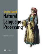
In the list that follows, let’s summarize what might have gone wrong with the simple lexicon-based approach and what can be improved (figure 8.1 visualizes the mental model for this chapter).
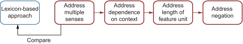
Figure 8.1 Mental model for the improved sentiment analysis implementation
-
Words may change their polarity and strength of sentiment across domains as well as over time. For instance, soft is not a very positive quality to have in sports (e.g., soft player), but it would sound positive in many other domains (e.g., when talking about clothes as in soft pajamas). The SocialSent lexicons that you used in the previous chapter solve these issues to a certain extent, as there is a range of lexicons built per domain and decade. However, one remaining problem is that the same word can have several meanings, which may in turn be associated with different sentiments. For instance, terrific has gradually changed its meaning and sentiment from negative (something scary and terrifying) to pretty positive (something impressive and on a grand scale) sometime between 1800 and the 2000s, so the more up-to-date versions of the lexicons contain a positive score for it. At the same time, the lexicons contain a single score for each word only, but a resource that can help you distinguish between more subtle differences in meaning and associated sentiment scores might provide you with better results. After all, there is always a chance that someone would still use terrific in this very old negative sense. We will refer to this case as multiple senses of the word issue and will look into how to improve this aspect of the system.
-
A lot depends on the surrounding context of the word. We’ve talked about examples of contexts that are overall positive (e.g., “Just go see this movie”) or negative (e.g., “How could anyone sit through this movie?”) without containing a single strong polarity word. It’s the combination of words, then, that makes the whole phrase or sentence sentiment-bearing. We will refer to this case as a dependence on context issue. A static resource like a sentiment lexicon cannot make subtle context-specific distinctions, and here is where a data-driven approach, with the classifier learning directly from the data, is more promising. In this chapter, you will put this hypothesis to the test.
-
Sometimes, looking at the words on their own is not enough. For instance, a cheap rate may express a positive sentiment, while a cheap trick denotes something quite negative. Related to this is the observation that it would be hard to spot irony, sarcasm, and metaphorical use of a word (as in “Otherwise, it's pretty much a sunken ship of a movie”) if you always looked at a single word at a time. We will refer to this as the length of the sentiment-bearing unit issue and will look into how to handle this in a machine-learning classifier.
-
The final issue, which is in a way related to the previous one, is the case of negation. In the previous chapter, we identified a group of words that have a special effect on the surrounding context—specifically, they have the ability to change the sentiment of what follows. For instance, neither super nor standard or nothing spectacular convert positive phrases into negative ones, while not bad puts the description on the positive scale.
Using the results of the sentiment lexicon-based system built in chapter 7 as the benchmark and involving machine-learning techniques and data-driven approaches, in this chapter you will try to improve your sentiment analyzer step-by-step.
8.1 Addressing multiple senses of a word with SentiWordNet
Our discussion about the sentiment detection based on a sentiment resource wouldn’t be complete without talking about SentiWordNet, a lexical database where different senses of a word are assigned with different sentiment scores. Since language is diverse and creative, using a resource that accounts for the sentiment difference of various instances of the word use is preferable to relying on a single score resource. In what cases should you care about that?
In previous chapters, we talked about parts of speech and how identification of the part of speech helps make (the right) sense of expressions like “I saw her duck” (figure 8.2 shows a reminder).

Figure 8.2 The two senses of the word duck, as a verb (to move downward) and as a noun (bird)
In this case, applying part-of-speech tagging, as you did in various previous applications, would help distinguish between the two options. In other situations, things go a step further: a classic, widely used example in NLP domain is the case of bank. How many possible readings of the word bank can you think of? Here are the two most common contexts of use:
In the first case, one is talking about a bank as a financial institution, while in the second it is the riverbank that one has in mind. Both cases of bank belong to the same part of speech (they are nouns), and the best clues as to what is meant in each sentence are the words surrounding bank: such as the references to money in the first sentence, and the references to water in the second. So far so good, but what about such sentences as “I went to the bank”? In which sense is bank used here? Our intuition tells us that, most probably, in everyday life we’d hear this statement from someone who is going to a bank to get some money. However, in general, this sentence is naturally ambiguous and may well mean that someone went fishing on a riverbank. Language is full of such ambiguities.
Why is this relevant to our task at hand? If a word may mean different things, each of these things may be positive or negative to a different extent independently of other senses of the same word. A resource that can tell you about such differences in meaning and sentiment is of a great value. Luckily, such a resource exists: it is called SentiWordNet (http://mng.bz/YG4Q) by analogy with a widely used lexical database called WordNet (https://wordnet.princeton.edu), to which it is closely related.
WordNet is a lexical database created at Princeton University, and it is an invaluable resource to use with any application that recognizes that words can be ambiguous between various senses. Essentially, WordNet is a huge network containing various nouns, verbs, adjectives, and adverbs grouped into sets of cognitive synonyms (i.e., words that mean similar things in the same context, as in interesting film = interesting movie or fast car = fast automobile). Such groups of cognitive synonyms in WordNet are called synsets. For instance, one such synset in WordNet would contain both words {film, movie} (and another one both words {car, automobile}) and that suggests that the words within each of these groups can be used interchangeably in various contexts. In total, there are 117,000 such groups of interchangeable words—that is, 117,000 synsets—and they also hold certain further relations among themselves. For instance, WordNet imposes a hierarchy on concepts, so you can also link them via the IS-A relation; for example, {car, automobile} is a type of vehicle (i.e., car/automobile IS-A vehicle), and {film, movie} is a type of show (i.e., film/ movie IS-A show), which is, in turn, a type of event, and so on. We are not going to discuss such other relations in detail in this chapter, since it is the synonymy relation, the one that holds the words within each synset together, that is most relevant for sentiment analysis.
To use a concrete example, let’s look into how terrific is represented in WordNet. WordNet distinguishes between three senses of the word:
Figure 8.3 visualizes the three synsets and includes definitions, further words belonging to each of these synsets, and examples of use (the WordNet interface, where you can search for words and their synsets, is available at http://mng.bz/Pnw9).

Figure 8.3 Three synsets for terrific, with definitions, other words from the same synset, and examples
One would expect the first two synsets (i.e., each of the words covered by these synsets) to carry a positive sentiment, and the third one to be negative. This is, in essence, the motivation behind SentiWordNet (https://github.com/aesuli/SentiWordNet), a sentiment-oriented extension to WordNet, developed by the researchers from the Text Learning Group at the University of Pisa.
SentiWordNet closely follows the structure of WordNet itself. That is, the same synsets are included in SentiWordNet, and each one is assigned with three scores: a positive score, a negative score, and an objective (neutral) score. The scores are assigned by a “committee” of classifiers—a combination of eight different machine-learning classifiers, where each one votes for one of the three polarity dimensions (find more details on implementation at http://mng.bz/GE58). In the end, the votes for each dimension (positive, negative, and objective) are aggregated across the classifiers and the scores represent the proportion of the classifiers among the eight that vote for the score of a particular polarity.
A nice fact about these two resources is that they are easily accessible through an NLTK interface. You used NLTK resources earlier in this book, such as when you accessed the texts from Project Gutenberg in chapters 5 and 6. You are going to use a similar approach here. Open your Jupyter Notebook that you worked on in chapter 7. You will add to that throughout this chapter.
Listing 8.1 shows how to access SentiWordNet via NLTK and check how two words, joy and trouble, are represented in WordNet. First, import sentiwordnet from NLTK and give it a shortcut for brevity. Next, you check which synsets words of your choice belong to. In this example, I check joy and trouble.
Note In addition to the toolkit itself, you need to install NLTK data as explained at www.nltk.org/data.html. Running nltk.download() will install all the data needed for text processing in one go; in addition, individual tools can be installed separately; for example, nltk.download('sentiwordnet') installs SentiWordNet.
Listing 8.1 Code to access SentiWordNet and check individual words
import nltk
nltk.download('wordnet')
nltk.download('sentiwordnet')                   ❶
from nltk.corpus import sentiwordnet as swn     ❷

print(list(swn.senti_synsets('joy')))
print(list(swn.senti_synsets('trouble')))       ❸
❶ Install NLTK’s interfaces to WordNet and SentiWordNet.
❷ Import sentiwordnet from NLTK and give it a shortcut for brevity.
❸ Check which synsets words of your choice belong to.
The code produces the following output:
[SentiSynset('joy.n.01'), SentiSynset('joy.n.02'), SentiSynset('rejoice.v.01'), SentiSynset('gladden.v.01')]
[SentiSynset('trouble.n.01'), SentiSynset('fuss.n.02'), SentiSynset('trouble.n.03'), SentiSynset('trouble.n.04'), SentiSynset('worry.n.02'), SentiSynset('trouble.n.06'), SentiSynset('disturb.v.01'), SentiSynset('trouble.v.02'), SentiSynset('perturb.v.01'), SentiSynset('trouble_oneself.v.01'), SentiSynset('trouble.v.05')]
This shows that joy may be a noun (the synset 'joy.n.01', meaning the “emotion of great happiness,” or the synset 'joy.n.02', meaning “something/someone providing a source of happiness as in “a joy to behold”). Alternatively, joy may be a verb, and as a verb, it can mean “rejoice” (“feel happiness or joy” [synset 'rejoice.v.01']) or “gladden” (“make glad or happy” [synset 'gladden.v.01']). You can tell which part of speech is involved by the abbreviations: e.g., n for noun and v for verb.
Trouble is a more complex case, with as many as six different meanings as a noun. For instance, it can mean a particular event causing pain, as in “heart trouble,” or a difficulty, as in “he went to a lot of trouble,” and as many as five senses for the verb. The differences may be quite subtle, yet leading to different interpretations, potentially with sentiments of different strength.
Let’s check this out. With the code from listing 8.2, you can check the positive and negative scores assigned in SentiWordNet to various senses of the words you choose. The following code accesses two synsets for joy and two synsets for trouble. With this code, you can access specific synsets (senses) for each of the input words (feel free to use different words) and use the printout routine from the previous chapters to print the results as a table. Each synset has a positive and a negative score assigned to it. You can access them with pos_score() and neg_score().
Listing 8.2 Code to explore the differences in the sentiment scores for word senses
joy1 = swn.senti_synset('joy.n.01')
joy2 = swn.senti_synset('joy.n.02')

trouble1 = swn.senti_synset('trouble.n.03')
trouble2 = swn.senti_synset('trouble.n.04')                         ❶


categories = ["Joy1", "Joy2", "Trouble1", "Trouble2"]
rows = []
rows.append(["List", "Positive score", "Negative Score"])           ❷
accs = {}
accs["Joy1"] = [joy1.pos_score(), joy1.neg_score()]
accs["Joy2"] = [joy2.pos_score(), joy2.neg_score()]
accs["Trouble1"] = [trouble1.pos_score(), trouble1.neg_score()]
accs["Trouble2"] = [trouble2.pos_score(), trouble2.neg_score()]     ❸
for cat in categories:
    rows.append([cat, f"{accs.get(cat)[0]:.3f}",
                f"{accs.get(cat)[1]:.3f}"])

columns = zip(*rows)
column_widths = [max(len(item) for item in col) for col in columns]
for row in rows:
    print(''.join(' {:{width}} '.format(row[i], width=column_widths[i])
                  for i in range(0, len(row))))                     ❹
❶ Access specific synsets (senses) for each of the input words.
❷ Use the printout routine from the previous chapters to print the results as a table.
❸ Each synset has a positive pos_score() and a negative neg_score() assigned to it.
❹ Print positive and negative scores for each synset.
Table 8.1 Results printed out by the code from listing 8.2
In other words, despite both senses of joy (as an emotion and as a source of happiness) being overall positive, the first one, the emotion, is more ambiguous between the positive and negative uses, as 50% of the classifiers (4 out of 8) voted for the positive sentiment, and 25% (2 out of 8) voted for the negative sentiment, with the rest voting for the neutral sentiment for this sense of the word. The second sense of joy is more markedly positive, with 37.5% (3 out of 8 of the classifiers) voting for the positive sentiment, and the rest for the neutral one. Note that the two senses of trouble (as an event causing pain or as a difficulty) are decidedly negative, but even here the degree of negativity is different.
As you can see, different senses of the same word are indeed marked with sentiments of different strength, if not of different polarity. Ideally, when encountering a word in text, you would like to first detect which sense it is used in and then access the sentiment scores for that particular sense. In practice, this first step, called word sense disambiguation (see Section 18.4 in https://web.stanford.edu/~jurafsky/slp3/18.pdf) is a challenging NLP task in its own right. Short of attempting full-scale word sense disambiguation, in this chapter we are going to detect the part of speech for the word (e.g., trouble as a noun) and extract the sentiment scores pertaining to the senses of this word when it is used as this part of speech (i.e., only noun-related sentiment scores for trouble will be taken into account). This will help you eliminate at least one level of word ambiguity.
Listing 8.3 shows how to access synsets related to the specific part of speech for a given input word. For example, nouns can be accessed with tag n or wn.NOUN, verbs with v or wn.VERB, adjectives with a or wn.ADJ, and adverbs with r or wn.ADV. As this code shows, you can access synsets for a given word (e.g., terrific) of a specific part of speech (e.g., adjective) using an additional argument with the senti_synsets function. In the end, you print out positive and negative scores for each synset, using + and - in front of the scores for clarity, as by default all scores are returned as absolute values without indication of their polarity.
Listing 8.3 Code to access synsets of a specific part of speech
synsets = swn.senti_synsets('terrific', 'a')      ❶
for synset in synsets:
    print("pos: +" + str(synset.pos_score()) +
          " neg: -" + str(synset.neg_score()))    ❷
❶ Access synsets for a given word of a specific part of speech using an additional argument in senti_synsets.
❷ Print out positive and negative scores for each synset.
This code produces the following output:
pos: +0.25 neg: -0.25
pos: +0.75 neg: -0.0
pos: +0.0 neg: -0.625
That is, out of the three senses of terrific, the second one associated with “extraordinarily good or great” is strongly positive (+0.75 for positive), the third one associated with “causing extreme terror” is strongly negative (-0.625 for negative), and the first one associated with “very great or intense” is ambiguous between the two polarities—it can be treated both as positive (+0.25) and negative (-0.25). It looks like intensity may not always be welcome; after all, something like “a terrific noise” may elicit negative or positive emotions, and SentiWordNet captures this idea. Figure 8.4 visualises this further.

Figure 8.4 Three synsets of terrific with different sentiment scores assigned to them
Now let’s see how you can incorporate the SentiWordNet information with your sentiment analyzer. As in listing 8.3, let’s make sure that you are accessing the right type of synsets—that is, let’s extract the synsets for the specific part of speech. Remember that you have previously (i.e., while building your baseline classifier in chapter 7) processed the reviews with spaCy and saved the results in the linguistic containers pos_docs and neg_docs. These containers, among other information, contain POS tags for all words in the reviews. You don’t need to run any further analysis to detect parts of speech, but the particular tags used to denote each part of speech differ between spaCy and NLTK’s interface to SentiWordNet. Here is the summary of the differences:
-
Nouns have tags starting with NN in spaCy’s notation and are denoted as wn.NOUN in NLTK’s interfaces to WordNet and SentiWordNet. (For the full tag description, check the English tab under Part-of-Speech Tagging at https://spacy.io/usage/linguistic-features#pos-tagging.)
-
Verbs have tags starting with VB or MD in spaCy and are denoted as wn.VERB in NLTK.
-
Adjectives have tags starting with JJ in spaCy and are denoted as wn.ADJ in NLTK.
-
Adverbs have tags starting with RB in spaCy and are denoted as wn.ADV in NLTK.
Note that only these four parts of speech are covered by WordNet and SentiWordNet, so it would suffice to take only words of these four types into account. Listing 8.4 first implements the convert_tags function that translates POS tags between two toolkits and then returns a predicted label for a review based on the aggregation of positive and negative scores assigned to each synset to which the word may belong. Specifically, in this code, for each word token in the review, you check whether it is an adjective, an adverb, a noun, or a verb based on its POS tag. Then you retrieve the SentiWordNet synsets based on the lemma of the word and its POS tag. The score is aggregated as the balance between the positive and negative scores assigned to each synset for the word token. Finally, you return the list of decisions, where each item maps the predicted score to the actual one.
Listing 8.4 Code to aggregate sentiment scores based on SentiWordNet
from nltk.corpus import wordnet as wn                                        ❶

def convert_tags(pos_tag):
    if pos_tag.startswith("JJ"):
         return wn.ADJ
    elif pos_tag.startswith("NN"):
         return wn.NOUN
    elif pos_tag.startswith("RB"):
         return wn.ADV
    elif pos_tag.startswith("VB") or pos_tag.startswith("MD"):
         return wn.VERB
    return None                                                              ❷

def swn_decisions(a_dict, label):
    decisions = []
    for rev_id in a_dict.keys():
        score = 0
        neg_count = 0
        pos_count = 0
        for token in a_dict.get(rev_id):
            wn_tag = convert_tags(token.tag_)
            if wn_tag in (wn.ADJ, wn.ADV,
                          wn.NOUN, wn.VERB):                                 ❸
                synsets = list(swn.senti_synsets(
                    token.lemma_, pos=wn_tag))                               ❹
                if len(synsets)>0:
                    temp_score = 0.0
                    for synset in synsets:
                        temp_score += synset.pos_score() - synset.neg_score()❺

                    score += temp_score/len(synsets)
        if score < 0:
            decisions.append((-1, label))
        else:
            decisions.append((1, label))
    return decisions                                                         ❻
❶ Import WordNet interface from NLTK for part-of-speech tag conversion.
❷ Function convert_tags translates between the tags used in the two toolkits.
❸ For each word token in the review, check its part-of-speech tag.
❹ Retrieve the SentiWordNet synsets based on the lemma of the word and its part-of-speech tag.
❺ Aggregate the score as the balance between the positive and negative scores of the word synsets.
❻ As before, return the list of decisions, where each item maps the predicted score to the actual one.
Figure 8.5 visualizes the process of aggregating scores derived from SentiWordNet with a short example of a review consisting of a single phrase: “The movie was terrific!” First, POS tags for all words in the review are extracted from the linguistic containers. In this example, “The” is the determiner (tag DT), and “!” is a punctuation mark (tag “.”). They are not considered further by the pipeline, and their tags are not converted to the WordNet ones, because WordNet doesn’t cover these parts of speech. Other words—“movie” (tag NN), “was” (tag VBD), and “terrific” (tag JJ)—are considered further, and their tags are converted into wn.NOUN, wn.VERB, and wn.ADJ by the convert_tags function. Next, synsets are extracted from SentiWordNet applying swn.senti_synsets to (“movie”, wn.NOUN), (“be”, wn.VERB), and (“terrific”, wn.ADJ). This function returns
-
One synset for “movie” with scores (+0.0, -0.0); that is, it is a very unambiguous and a totally neutral word.
-
As many as 13 synsets for “be,” 11 of which are neural with scores (+0.0, -0.0), one mostly positive with scores (+0.25, -0.125), and one neutral on balance with scores (+0.125, -0.125).
-
Three synsets for “terrific” that we’ve just looked into (see figure 8.4).

Figure 8.5 An example of how the scores are aggregated using the code from listing 8.4
Without prior word sense detection, it is impossible to say in which sense each of the words is used, but you can take into account the distribution of all possible sentiments across senses and rely on the idea that, overall, the accumulated score will reflect possible deviations in sentiment. For instance, an overwhelmingly positive word that is positive in all its senses will get a higher score than a word that may be used in a negative sense once in a while. So, for example, if you sum up all sentiment scores across all synsets for “terrific,” you’ll get (0.25 - 0.25 + 0.75 - 0.0 + 0.0 - 0.625) = 0.125. The final score is still positive, but it is lower than the positive scores in some of its synsets (0.25 and 0.75) because it may also have a negativity component to it (-0.25 or even -0.625).
Once you’ve accumulated scores across all synsets of a word for each of the words in the review, the final score, as before, is an aggregation of the individual word scores. For this short review, it is 0.25, meaning that the review is quite positive. For convenience, the code in listing 8.4 converts all positive predictions into label 1 and all negative ones into -1.
Finally, let’s compare the results produced by this approach to the actual sentiment labels. As before, let’s calculate the accuracy of prediction by comparing the predicted scores (1 and -1) to the actual scores (1 and -1) and estimating the proportion of times your predictions are correct. Listing 8.5 implements this evaluation step in a similar manner to the evaluation in the previous chapter. In this code, you first extract and save the label predictions for the pos_docs (positive reviews with the actual label 1) and for neg_docs (negative reviews with the actual label -1) in two data structures. Next, you detect a match when the predicted score equals the actual score and calculate the accuracy as the proportion of cases where the predicted score matches the actual one. Finally, you print out the results as a table using the printing routine from before.
Listing 8.5 Code to evaluate the results for this approach
def get_swn_accuracy(pos_docs, neg_docs):
    decisions_pos = swn_decisions(pos_docs, 1)
    decisions_neg = swn_decisions(neg_docs, -1)              ❶
    decisions_all = decisions_pos + decisions_neg
    lists = [decisions_pos, decisions_neg, decisions_all]
    accuracies = []
    for i in range(0, len(lists)):
        match = 0
        for item in lists[i]:
            if item[0]==item[1]:                             ❷
                match += 1
        accuracies.append(float(match)/
                          float(len(lists[i])))              ❸
    return accuracies


accuracies = get_swn_accuracy(pos_docs, neg_docs)

rows = []
rows.append(["List", "Acc(positive)", "Acc(negative)", "Acc(all)"])
rows.append(["SentiWordNet", f"{accuracies[0]:.6f}",
                f"{accuracies[1]:.6f}",
                f"{accuracies[2]:.6f}"])

columns = zip(*rows)
column_widths = [max(len(item) for item in col) for col in columns]
for row in rows:
    print(''.join(' {:{width}} '.format(row[i], width=column_widths[i])
                  for i in range(0, len(row))))              ❹
❶ Save the label predictions for the pos_docs and neg_docs.
❷ When the predicted score equals the actual score, consider it a match.
❸ Accuracy reflects the proportion of cases where the predicted score matches the actual one.
❹ As before, print out the results as a table using the printing routine.
This code returns the results shown in table 8.2.
Note As in other examples, you might end up with slightly different results if you are using versions of the tools different from those suggested in the installation instructions for the book. In such cases, you shouldn’t worry about the slight deviations in the numbers as the general logic of the examples still holds.
Table 8.2 Results returned by the code from listing 8.5
In other words, this method achieves an overall accuracy of 68.80% and performs almost equally well on both positive and negative reviews. This is a clear improvement over the results obtained with your first, baseline classifier. To conclude this part of the chapter, let’s visualize the results. Figure 8.6 presents the best accuracy of your baseline lexicon-based model (64.75%) in comparison with the current results (68.80%), with the majority class baseline for this dataset being 50%.

Figure 8.6 Accuracies achieved by two methods applied so far—lexicon-based and SentiWordNet-based
8.2 Addressing dependence on context with machine learning
The results that you’ve obtained before with the simple sentiment lexicon-based approach and the advanced approach based on SentiWordNet, which allows you to adjust the sentiment score of a word based on the distribution of sentiment across its senses, still leave room for improvement. Given that a random choice of a sentiment label would be correct half of the time (since the distribution of labels is 50/50), the best accuracy you can get with a lexicon-based approach, using adjectives only, is about 0.65, and you reach around 0.69 with the SentiWordNet approach. Admittedly, the authors of the original paper cite similar accuracy figures (www.cs.cornell.edu/home/llee/papers/sentiment.pdf) for a simple lexicon-based approach that they applied. Still, their best results that they report on this task are quite a bit higher: their machine-learning models use a range of features and achieve accuracy values from around 78% up to about 83%. Even though the dataset you are working with is a slightly different version of the data (this paper used a smaller subset of 700 positive and 700 negative reviews from the same data), and it would, strictly speaking, be unfair to compare the performance on different datasets, the results in the region of 78% to 83% should provide you with a general idea of what is possible to achieve on this task. So how can you do better?
One aspect that your algorithm is currently not taking into account is the exact data you are working with. Even though you haven’t yet been using a data-driven approach or machine-learning methods on this task yourself, you have already been using the product of such methods applied to this task, as both sentiment lexicons and SentiWordNet were, in fact, created using machine-learning and data-driven approaches. That means that they have potentially captured a lot of useful information about many words in language; however, there might still be a mismatch between how those words were used in their data and what you have in your reviews dataset. You are now going to look into the next challenge in sentiment analysis—dependence of word sentiment on the surrounding context—and you are going to learn the word sentiment dynamically based on the data at hand. It’s time now to revisit approach 2 that we formulated in chapter 7:
Figure 8.7 is a reminder on the machine-learning pipeline as applied to the sentiment data.

Figure 8.7 Machine-learning pipeline applied to the sentiment data
8.2.1 Data preparation
We are going to turn to scikit-learn now and use its functionality to prepare the data, extract features, and apply machine-learning algorithms. The first step in the process, as figure 8.7 visualizes, is preparing the texts from the dataset for classification. So far you have been working with two dictionaries: pos_docs, which store all positive reviews’ IDs mapped to the content extracted from the correspondent files and processed with spaCy, and neg_docs, which store all negative reviews’ IDs mapped to the linguistically processed content. The spaCy’s linguistic pipeline adds all sorts of information to the original word tokens (e.g., earlier in this chapter you’ve used lemmas and POS tags retrieved from pos_docs and neg_docs). It’s time now to decide which of these bits of information to use in your machine-learning application as features. In particular, you need to consider the following questions:
-
Question 1—Are all words equally important for this task? For some other applications in the previous chapters, you removed certain types of words (e.g., stopwords). In addition, in chapter 7 you saw that words of certain parts of speech (e.g., adjectives or adverbs) might be more useful than others. Should you take all words into account, or should you do some prefiltering of the content?
-
Question 2—What should be used as features for the classification? Is it word forms, so that film and films would give rise to two different features in the feature vector, or is it lemmas so that both would result in a single feature “film”? Should you consider single words like very and interesting, or should you take phrases like very interesting into account too?
These are reasonable questions to ask yourself whenever you are working on an NLP classification task. Regarding question 1, you might have noticed that none of the sentiment lexicons contained words like a or the (called articles), of or in (called prepositions), and other similar frequent words that are commonly called stopwords. In fact, the researchers who compiled these lists specified that stopwords were filtered out. SentiWordNet doesn’t cover such words either. On the one hand, since stopwords mainly help link other words together (as prepositions do) or add some aspects to the meaning (as the indefinite article a or definite article the do), many of them don’t express any sentiment value in addition to this main function of linking other words to each other, so you might consider filtering them out.
On the other hand, care should be taken as to what words are included in the list of stopwords: for instance, traditionally negative words like not and similar are also considered stopwords, but as you’ve seen before, they are useful for sentiment detection. You might have also noticed that lexicons and SentiWordNet do not contain any punctuation marks. Whether to include punctuation marks in the set of features is another choice you’ll have to make. On the one hand, emotional statements often contain special punctuation such as exclamation marks, making them potentially useful as a feature. However, on the other hand, both positive (“This movie is a must-see!”) and negative (“Don’t waste your time on this movie!”) reviews may contain them, making such punctuation marks less discriminative as a feature. To this end, let’s implement a flexible filtering method, text_filter, that will allow you to customize the list of words that you’d like to ignore in processing. After filtering is done, let’s consider all other words as potential features. Once you get the results with the full vocabulary, you will be able to compare the performance to the more limited sets of features (e.g., adjectives only). To see how the original content of a review may get dramatically distilled by the text_filter method down to content words, take a look at figure 8.8.

Figure 8.8 The content of the original review filtered down by a text_filter method
Question 2 asks you which linguistic unit should be used as the basis for the features. Recall that one of the challenges in sentiment analysis identified in the beginning of this chapter is the size of the feature unit. This is not a completely novel question for you. Recall that in chapters 5 and 6, you used units smaller than a word (suffixes of up to three characters in length) to classify texts as belonging to one of the authors. Although you can consider units shorter than a word as features for sentiment analysis, too, traditionally words are considered more suitable as features for this application. Use of lemmas instead of word forms will make your feature space more compact as you’ve seen during the data exploration phase; however, you might lose some sentiment-related information through this space-reduction step (e.g., word form worst might bear a stronger sentiment clue than its lemma bad). You might have also noticed that the sentiment lexicons used in the previous chapter contain word forms rather than lemmas. Again, let’s make sure that the filtering method, text_filter, is flexible enough to allow you to change the level of granularity for your features if needed.
Finally, if you look into previous research on sentiment analysis—for instance, into the seminal paper “Thumbs Up? Sentiment Classification using Machine Learning Techniques” that accompanied the reviews dataset—sentiment analysis algorithms often consider units longer than single words as features. In particular, the paper mentions using word bigrams as well as unigrams as features. What does this mean?
If you continue working in NLP, you will come across such terms as unigrams, bigrams, trigrams, and n-grams in general very often. These terms define the length of a particular linguistic unit, typically in terms of characters or words. For example, character n-grams specify the length of a sequence of characters, with n- in n-gram standing for the length itself. Figure 8.9 illustrates how to identify n-grams of a specific length in terms of characters and words.

Figure 8.9 Identification of n-grams of various length n in terms of characters and words
In fact, one of the feature types used for author identification in chapters 5 and 6—suffixes—can be considered an example of character trigrams. Let’s give it a proper definition.
When thinking of using word n-grams as features for sentiment analysis, ask yourself whether word unigrams (e.g., very, good, and movie extracted from “Very good movie”) are sufficiently informative, or whether addition of the word bigrams “very good” and “good movie” to the feature space will help the classifier learn the sentiment better. There is a certain tradeoff between the two options here. While bigrams might add some useful signal to the feature space, there are advantages to sticking to unigrams only. In particular:
-
A word unigrams-based feature space is always more compact—For example, if you have 100 word unigrams, theoretically there may be up to 100*100 = 10,000 bigrams—a very significant increase in the feature space size and a toll on the algorithm’s efficiency.
-
A word unigrams-based feature space is always less sparse—Imagine that you’ve seen very 50 times and good 100 times, and you are quite certain that very doesn’t always occur in combination with good. How often, then, will you see “very good” in this data? You can be sure, this will be less than 50 times (i.e., the lower frequency of the words within an n-gram always sets up the upper bound on the frequency of the word combination as a whole), and the longer the n-gram becomes, the less often you will see it in the data. This might eventually mean that the n-gram becomes too rare to be useful in classification.
We will get to the question of using longer word n-grams, as well as a combination of uni- and longer n-grams a little later in this chapter once you get more familiar with the scikit-learn’s functionality. Right now, let’s get straight to coding and implement two functions that will allow you to apply filtering of your choice to the content of the reviews and will help you prepare the data for further feature extraction. Listing 8.6 does exactly that, filtering out punctuation marks and keeping word forms. Feel free to experiment with other types of filtering.
In this code, you start by adding some useful imports: random for data shuffling, string to access the list of punctuation marks, and finally, spaCy’s stopwords list. We’ll use the standard list of punctuation marks. Note that string.punctuation is a string of punctuation marks, so let’s convert it to a list for convenience. Alternatively, you can define your own customized list instead. Next, you pass in a reviews dictionary a_dict, where each review’s ID is mapped to its content, a label (1 for positive and -1 for negative reviews) and exclude_lists for the lists of words to be filtered out as arguments to the function text_filter. For the word forms that are not in the exclude_lists, you add the word forms to the output. Alternatively, you can use token.lemma_ instead of token.text in this code to take lemmas instead of word forms. You return data—a data structure with tuples, where the first element in each tuple is a filtered down version of a review and the second is its label. After that, you apply the text_filter function to both types of reviews and put the tuples of filtered reviews with their labels together in one data structure. Within the prepare_data function, you shuffle the data entries randomly, and to ensure that this random shuffle results in the same order of reviews from one run of your system to another, you set a random seed (e.g., 42 here). Then you split the randomly shuffled tuples into two lists: texts for the filtered content of the reviews and labels for their labels. This code shows how to filter out punctuation marks using the prepare_data function. For both punctuation and stopwords filtering, you’ll need to use list(stopwords_list) + punctuation_list. In the end, you apply the prepare_data function to the dataset and print out the length of the data structures (this should equal the original number—2,000 reviews here), as well as some selected text (e.g., the first one texts[0]).
Listing 8.6 Code to filter the content of the reviews and prepare it for feature extraction
import random                                                       ❶
import string
from spacy.lang.en.stop_words import STOP_WORDS as stopwords_list
punctuation_list = [punct for punct in string.punctuation]          ❷

def text_filter(a_dict, label, exclude_lists):                      ❸
    data = []
    for rev_id in a_dict.keys():
        tokens = []
        for token in a_dict.get(rev_id):
            if not token.text in exclude_lists:
                tokens.append(token.text)                           ❹
        data.append((' '.join(tokens), label))
    return data                                                     ❺

def prepare_data(pos_docs, neg_docs, exclude_lists):
    data = text_filter(pos_docs, 1, exclude_lists)
    data += text_filter(neg_docs, -1, exclude_lists)                ❻
    random.seed(42)
    random.shuffle(data)                                            ❼
    texts = []
    labels = []
    for item in data:
        texts.append(item[0])
        labels.append(item[1])
    return texts, labels                                            ❽

texts, labels = prepare_data(pos_docs, neg_docs, punctuation_list)  ❾

print(len(texts), len(labels))
print(texts[0])                                                     ❿
❷ string.punctuation is a string of punctuation marks, so let’s convert it to a list for convenience.
❸ Pass in a_dict, a label, and exclude_lists as arguments.
❹ For the word forms that are not in the exclude_lists, add the word forms to the output.
❺ Return data, with the first element being a filtered down version of a review, and the second its label.
❻ Apply the text_filter function to both types of reviews and store the results in one data structure.
❼ Shuffle the data entries randomly.
❽ Split the randomly shuffled tuples into two lists—texts and labels.
❾ Filter out punctuation marks.
❿ Apply prepare_data function to the dataset and print out some results.
This code will print out 2,000 for the length of the texts list (i.e., the list of texts that represent filtered down content of each of the original reviews) and the length of the labels list (i.e., the list of labels, including 1 for a positive sentiment and -1 for a negative sentiment). These structures hold the processed data from the original 2,000 reviews.
To check how the data is now represented in the texts list, you use print(texts[0]) to peek into the first review in this structure. It corresponds to the positive review stored in the file cv795_10122.txt, the one used in the example in figure 8.8. Here is how the content looks now, with only the punctuation marks filtered out:
the central focus of michael winterbottom 's welcome to sarajevo is sarajevo itself the city under siege and its different effect on the characters unfortunate enough to be stuck there it proves the backdrop for a stunningly realized story which refreshingly strays from mythic portents [...]
Now let’s split this data into the usual subsets—the training set that you will use to make the classifier learn how to perform the task and the test set that you will use to evaluate the performance of the classifier (i.e., estimate how well it learned to perform the task at hand). Figure 8.10 highlights where you currently are in the machine-learning pipeline.

Figure 8.10 Next step in the machine-learning pipeline—split the data into the training and test sets
Let’s use a simple strategy: since you’ve already shuffled the data, the instances with different labels should be randomly ordered in texts and labels data structures, so you can allocate the first 80% of these instances to the training set and the other 20% to the test set. We are going to improve on this splitting strategy in a bit, so let’s not worry about further details of this random split for the moment. Listing 8.7 shows how to split the data into the texts for the training and test sets (called train_data and test_data) and labels for the training and test sets (train_targets and test_targets). Additionally, you can check that the data is randomly shuffled by printing out the first 10 labels from each of the subsets. Specifically, you implement the function split, which should split input lists of texts and labels into training and test set texts and labels using the predefined proportion. As the code suggests, you use 0.8 to allocate the first 80% of the input texts to the train_data and the first 80% of the input labels to the train_targets, while putting the other 20% of the input texts into the test_data and the other 20% of the input labels into the test_targets. Finally, you print out the length of each list as well as the labels for the first 10 items in the target lists.
Listing 8.7 Code to split the data into the training and test sets
def split(texts, labels, proportion):
    train_data = []
    train_targets = []
    test_data = []
    test_targets = []
    for i in range(0, len(texts)):
        if i < proportion*len(texts):
            train_data.append(texts[i])
            train_targets.append(labels[i])
        else:
            test_data.append(texts[i])
            test_targets.append(labels[i])
    return train_data, train_targets,
           test_data, test_targets                       ❶

train_data, train_targets, test_data, test_targets =
                           split(texts, labels, 0.8)     ❷

print(len(train_data))
print(len(train_targets))
print(len(test_data))
print(len(test_targets))
print(train_targets[:10])
print(test_targets[:10])                                 ❸
❶ The split function splits input lists of texts and labels into training and test sets using predefined proportion.
❷ Use the proportion 0.8 to allocate 80% of the data to the training set and 20% to the test set.
❸ Print out the length of each list as well as the labels for the first 10 items in the target lists.
If you run this code as is and use 80% of the texts and labels to train the classifier, you should get 1,600 for the length of the train_data and train_targets, and 400 for the length of the test_data and test_targets. Here’s the list of the first 10 labels from the training and the test data:
[1, -1, 1, 1, -1, -1, -1, -1, 1, -1]
[-1, 1, 1, -1, -1, 1, -1, 1, 1, 1]
This shows that positive reviews (label 1) are mixed with negative reviews (label -1) in a random order. Now you’ve done several preparation steps: you’ve prefiltered the content of the reviews to distill it down to what can be considered to constitute important features, you’ve separated texts from labels, and you’ve split the data into the training and the test sets. It’s time now to extract features and apply the full machine-learning pipeline, as figure 8.11 shows.

Figure 8.11 Next step in the machine-learning pipeline—extract features
8.2.2 Extracting features from text
One of the benefits of scikit-learn and, indeed, one of the reasons to use it in this book is that many steps in the machine-learning pipeline, such as feature extraction for NLP tasks, are made easy with this toolkit. One of the most widely used approaches to using words as features—in fact, the one that you’ve already used for some of the previous applications—is based on the idea that distribution of words contributes to the class prediction. For instance, if you see a word good used multiple times in a review, you would expect this review to express a positive sentiment overall. Similarly, if some negative words like bad or awful are simultaneously used in a review, it’s a strong signal that the review is overall negative. Therefore, if you have a list of words to estimate the distribution of in the data, your classifier can learn how frequently they occur in the positive and in the negative reviews. In fact, scikit-learn covers these two steps—collection of the vocabulary words to estimate distribution for and calculation of frequency of words from this vocabulary in each review—with a single tool called CountVectorizer.
Recall why you need to split the data into the training and test sets: when the algorithm learns how to solve the task, it sees only the data and labels from the training set. Based on that, it learns how to connect the data (features) from the training set to the labels, assuming that the training set represents the task at hand perfectly; that is, whatever the distribution of the features and their correspondence to the labels in the training data is, it will be exactly the same or very closely replicated in any future data you apply the trained algorithm to. When you apply it to the test data that the algorithm has not seen during its training, you can get a rough estimate of how the algorithm will perform on new, unseen data. Therefore, it is important that whatever the algorithm learns, it does so on the basis of the training data only, without peeking into the test set. To this end, the CountVectorizer does two things. First, it builds the vocabulary of words based on the training data only (which means that if some words occur in the test set only, they will be ignored during classification), and second, it estimates the correspondence between the feature distribution and the class label based on the training data only. The particular method that allows the CountVectorizer to do that is called fit_transform. Listing 8.8 shows how CountVectorizer can be applied to the training data. Behind the scenes, the fit_transform method from scikit-learn’s CountVectorizer extracts the shared vocabulary from all training set reviews and estimates frequency of each word from the vocabulary in each review. Once you’ve applied it to your data, you can print out the size of the train_counts data structure.
Listing 8.8 Code to apply CountVectorizer to learn the features on the training set
from sklearn.feature_extraction.text import CountVectorizer

count_vect = CountVectorizer()
train_counts = count_vect.fit_transform(train_data)    ❶

print(train_counts.shape)                              ❷
❶ The fit_transform method extracts the shared vocabulary from the training set and estimates word frequency.
❷ Let’s print out the size of the train_counts data structure.
This code produces the following output: (1600, 36094). What does this mean? The first element of the tuple tells you that the number of data entries in the training set equals 1,600. This is exactly the number of training set reviews. The second element is, in fact, the length of the collected vocabulary. This means that there are 36,094 distinct words in the vocabulary collected by the algorithm from all training set reviews. This vocabulary is then applied to each review to produce a feature vector, and the frequency of each word from this vocabulary is estimated for each review to fill in the values in this vector. You know from our statistical checks in the previous chapter that the average length of a review is about 800 words, and that is before punctuation marks or stopwords are filtered out. Obviously, no review will contain anything close to 36,094 distinct words in it. This means that the feature vectors will be extremely sparse (i.e., only a small portion of a vector will be filled with counts from the words that actually occur in the review, while the rest will be filled with 0s).
Let’s check this out. For instance, if you want to look “under the hood” of the algorithm and see what the CountVectorizer collected, you can use the following command:
print(train_counts[:11])
This will print out the counts collected for the first 10 reviews in the training set. In particular, it will print out the following:
(0, 32056)   41
(0, 5161)    1
(0, 12240)   1
(0, 22070)   18
...
The first element here tells you which review you are looking at. Index 0 means the first review from the training set—the one that starts with the central focus of . . . as printed out above and used in figure 8.8. The second element in each tuple tells you which word is used in a review by referring to its index from the alphabetically ordered vocabulary. For instance, the index 32056 corresponds to the word the, 5161 to the word central, 12240 to the word focus, and 22070 to the word of. You can always retrieve the word from the vocabulary by its index using count_vect.get_ feature_names()[index]. For instance, count_vect.get_feature_names()[35056] will return the.
Note In newer versions of scikit-learn, the get_feature_names() function is replaced with get_feature_names_out().
Finally, the printed-out numbers correspond to the number of occurrences of each word in the review. For example, in this review, the word the occurs 41 times, of 18 times, and the other two words discussed above occur only once.
Now, if you want to have a further look into the collected vocabulary, you can print it out using print(count_vect.get_feature_names()[:10]), which will print out the first 10 entries from the vocabulary:
['00', '000', '0009f', '007', '00s', '03', '04', '05', '05425', '10']
Finally, print(count_vect.vocabulary_) will print out the entries from the vocabulary mapped to their IDs:
{'the': 32056, 'central': 5161, 'focus': 12240, ...}Table 8.3 provides a glimpse into the vocabulary and feature vectors. The header presents the indexes from the vocabulary mapped to the words, while the figures show the frequency of each feature in the first review from the training set. Features that don’t occur in the review get a count of 0. The bottom row, therefore, shows you a small bit of the feature vector for the first review.
Table 8.3 A glimpse into the vocabulary and feature vectors
Now, let’s extract the same features from the test data and apply the classifier. In the previous chapters, you’ve learned that Naïve Bayes, unlike some other classifiers, can deal reasonably well with sparse features, such as distributions of words from a large vocabulary, where for each particular review only a few are present. To this end, let’s apply this classifier to your task. Figure 8.12 provides a reminder of the scikit-learn’s train-test routine and syntax.

Figure 8.12 A reminder of the scikit-learn’s train-test routine and syntax
Before you can apply a trained model to the test set, you need to extract the features from the test set, which is achieved in a very similar manner by applying the scikit-learn’s CountVectorizer. To make sure that the algorithm counts the occurrences of the words from the vocabulary that it collected from the training data only (rather than collecting a new vocabulary and counting word occurrences based on it), omit the call to the fit method of the vectorizer and use only the transform bit—that is, you are transforming the raw contents of the test set reviews to the feature vectors, without fitting them into a new vocabulary. Listing 8.9 walks you through these steps.
Listing 8.9 Code to apply CountVectorizer to test set and run classification
from sklearn.naive_bayes import MultinomialNB

clf = MultinomialNB().fit(train_counts, train_targets)    ❶

test_counts = count_vect.transform(test_data)             ❷
predicted = clf.predict(test_counts)                      ❸

for text, label in list(zip(test_data, predicted))[:10]:
    if label==1:
        print('%r => %s' % (text[:100], "pos"))
    else:
        print('%r => %s' % (text[:100], "neg"))           ❹
❶ Initialize the classifier and train the model on the training data using fit method.
❷ Extract features from the test data by applying the transform method of the CountVectorizer.
❸ Apply the classifier to make predictions on the test set.
❹ Print out some results, for example the predicted labels for the first 10 reviews from the test set.
This code will print out the first 100 characters from the first 10 reviews mapped with their predicted sentiment. Among them, you’ll see the following examples:
"susan granger 's review of america 's sweethearts columbia sony what a waste of a talented cast bill" => neg
'  the fugitive is probably one of the greatest thrillers ever made it takes realistic believable cha' => pos
This looks like a very sensible prediction; for instance, the word waste (as well as the whole phrase “a waste of a talented cast”) strongly suggests that it is a negative review, and the classifier picked that information up. The second review contains quite positive expressions, including “one of the greatest thrillers ever made” and “realistic believable cha[racters]”, thus the prediction made for this review is that it is positive.
Congratulations, you’ve just built a data-driven sentiment analyzer that is tuned to detecting sentiment based on your specific data! Now let’s look into how these multiple steps, including feature extraction and machine-learning classification, can be put together in a single flexible pipeline, and then let’s run a full-scale evaluation of the results.
8.2.3 Scikit-learn’s machine-learning pipeline
You’ve come across processing pipelines before, such as when you used the spaCy’s pipeline earlier in this chapter and in the previous chapters to apply all linguistic tools at once. Scikit-learn allows you to define your own pipeline of processing, feature extraction, and machine-learning tools as well. What’s the benefit of using such a pipeline? Here are the main advantages:
-
Once defined, you don’t need to worry about the sequence of tool application and consistency of the tools applied to training and test data. Define your pipeline once and then simply run it on any dataset.
-
Scikit-learn’s pipeline is highly customizable, and it allows you to bolt together various tools and subsequently run them with a single line of code (i.e., invoking the pipeline when needed). It makes it easy to experiment with different settings of the tools and find out what works best.
So, let’s find out how the pipeline works. Listing 8.10 shows how to define a pipeline. You start by importing the Pipeline functionality and the Binarizer tool, which helps record absence or presence of features. You can add any tools of your choice to the pipeline and print out the full list of tools included in it with the activated options. Once defined, the pipeline can be run using the usual fit-predict routine.
Listing 8.10 Code to define pipeline
from sklearn.pipeline import Pipeline          ❶
from sklearn.preprocessing import Binarizer    ❷

text_clf = Pipeline([('vect', CountVectorizer(min_df=10, max_df=0.5)),
                     ('binarizer', Binarizer()),
                     ('clf', MultinomialNB()),
                    ])                         ❸

text_clf.fit(train_data, train_targets)
print(text_clf)                                ❹
predicted = text_clf.predict(test_data)        ❺
❶ Import the Pipeline functionality.
❷ Import the Binarizer tool to record the absence or presence of features.
❸ Add any tools of your choice to the pipeline.
❹ You can print out the full list of tools included in the pipeline with the activated options.
❺ Apply the usual fit-predict routine.
Note that instead of defining the tools one by one and passing the output of one tool as the input to the next tool, you simply pack them up under the Pipeline, and after that you don’t need to worry anymore about the flow of the information between the bits of the pipeline. In other words, you can train the whole model applying fit method as before (which will use the whole set of tools this time) and then test it on the test set using predict method. Figure 8.13 is thus an update on figure 8.12.
Figure 8.13 Machine-learning routine using Pipeline functionality
Now let’s look more closely into the tools:
-
Previous applications of the CountVectorizer left the brackets empty, and this time we use some options: min_df=10 and max_df=0.5. What does this mean? (Check out the full list of available options at http://mng.bz/J2w0.) Recall from your earlier data explorations in this chapter that both positive and negative review collections have a large number of words in their vocabularies. The full vocabulary collected on the training set contains over 36,000 words, yet, as we’ve discussed, for any particular review the actual number of words occurring in it will be relatively small. The feature vectors of ~36,000 dimensionality are very expensive to create and process, especially given that they are very sparse (i.e., mostly filled with zeros for any given review). CountVectorizer allows you to mitigate this issue to some extent by setting cutoffs on the minimum and maximum document frequency (min_df and max_df options here). An integer value is treated as the absolute frequency, while a floating-point number denotes proportion of documents. By setting min_df to 10 and max_df to 0.5, you are asking the algorithm to populate only the vocabulary and count the frequency for the words that occur in more than 10 reviews in the training data and in no more than 800 of them (i.e., 0.5 of the 1,600 training reviews), thus eliminating some relatively rare words that might be not frequent enough to be useful, as well as some very frequent words that might be too widely spread to carry any useful information. This makes the feature space much more compact and often not only speeds up the processing but also improves the results (as in this case).
-
We are using a new tool, Binarizer, as part of this pipeline (check out the documentation at http://mng.bz/woZq). What does it do? Recall that with the lexicon-based approach, you tried two variations: taking absolute value of the sentiment (+1 for positive and -1 for negative words) or the relative sentiment weight. Binarizer allows you to do something a bit similar: it helps you to model the presence/absence of a word in a review as opposed to its frequency; in other words, it assigns a value of 1 (instead of a count) to each vocabulary word present in a review and a value of 0 to each vocabulary word absent from a review. The pipeline is very flexible in this respect. Add this tool to your pipeline and your classifier will rely on the presence/absence of features; remove it and your classifier will rely on frequencies. The authors of the “Thumbs Up?” paper report that presence/absence works better for sentiment analysis than frequency. Experiments on this version of the dataset show that the difference is very small, with presence/absence yielding slightly better results, so make sure you experiment with the different settings in the code.
Now, what are the results exactly? Let’s find out! Listing 8.11 reminds you how to evaluate the performance of your classifier (here, the whole pipeline) and print out a confusion matrix where the actual labels are printed against system’s predictions. Figure 8.14 shows a reminder of what information a confusion matrix contains.
Listing 8.11 Code to evaluate performance of your pipeline
from sklearn import metrics          ❶

print("
Confusion matrix:")
print(metrics.confusion_matrix(test_targets, predicted))
print(metrics.classification_report(
      test_targets, predicted))      ❷
❶ Import the collection of metrics.
❷ Print out the confusion matrix and the whole classification_report.

Figure 8.14 A reminder of what information is contained in the confusion matrix
Confusion matrix:
[[173  29]
 [ 41 157]]
              precision    recall  f1-score   support

          -1       0.81      0.86      0.83       202
           1       0.84      0.79      0.82       198

    accuracy                           0.82       400
   macro avg       0.83      0.82      0.82       400
weighted avg       0.83      0.82      0.82       400
A confusion matrix provides a concise summary of classifier performance (including both correctly classified instances and mistakes) and is particularly suitable for the analysis in binary classification cases. For instance, in this task you are classifying reviews into positive and negative ones. The example in figure 8.14 shows that in a set of 400 reviews (consisting of 202 actually negative reviews and 198 actually positive ones—you can estimate the totals following the numbers in each row), the classifier correctly identifies 173 negative and 157 positive ones. These numbers can be found on the diagonal of the confusion matrix. At the same time, the classifier incorrectly detects 29 negative reviews as positive, and 41 positive reviews as negative. The code in listing 8.11 reminds you how to print out the confusion matrix as well as the whole classification_report, which includes accuracy, precision, recall, and F-score for each class.
This particular pipeline run on this particular train-test split (with 202 negative and 198 positive reviews in the test set, as the support values show) achieves an accuracy of 82%, with a quite balanced performance on the two classes. In particular, it correctly classifies 173 negative reviews as negative and 157 positive reviews as positive; it incorrectly assigns a negative label to 41 actually positive reviews and a positive label to 29 actually negative ones. The last two lines of the report present macro average and weighted average for all metrics. You don’t need to worry about the difference between them, as for a balanced dataset (as the one you are using in this chapter), there is no difference between the two—they simply represent averages for the values in each column. The difference will show itself when the classes have unequal distribution. Weighted average will take the proportion of instances in each class into account, while macro average will average across all classes regardless.
Now that you know how to run a whole pipeline of tools in one go, attempt exercise 8.2. Try solving these tasks before checking the solutions in the Jupyter Notebook.
8.2.4 Full-scale evaluation with cross-validation
Now you’ve obtained some results on this dataset and they seem to be quite promising. The performance is rather balanced on the two classes; the accuracy of 0.82 is similar to that reported in the “Thumbs Up?” paper (recall that we’ve discussed earlier in this chapter that the authors report accuracy values in the region of 78% to 83% for this task on a subset of this dataset). Well done! There is just one caveat to consider before you declare success on this task. Remember that your train-test split comes from one specific way of shuffling the dataset (using a selected random seed, 42 in listing 8.6) and training on the first 80% and testing on the other 20% of it. What happens if you shuffle the data differently, for example, using a different seed?
You might guess that the results will change. They will indeed, and if you are interested further in this question, you can try this out as an experiment. The results might change ever so slightly, but still, they would be different. What’s more, you might also get “unlucky” with the new selection of the test set and get much lower results! Which results should you trust in the end? One way to make sure you get a fair range of results on different bits of the dataset, rather than on some random, perhaps some “lucky” test set (which might yield overly optimistic results), or perhaps some “unlucky” test set (that will make you believe the performance is lower than it actually is on another bit), is to run your classifier multiple times on different subsets of the data; for instance, changing the random seed and taking the mean of the results from multiple runs. How many times should you run your algorithm then?
In fact, there exists a widely used machine-learning technique called k-fold cross-validation that defines how such multiple runs of the algorithm over the data should be performed. K in the title of the technique stands for the number of splits in your data (and consequently also for the number of runs). Here is how you can apply k-fold cross-validation:
-
Split your full dataset into k random subsets (folds) of equal size. Traditionally, you would go for k = 5 or k = 10. Let’s assume that you decided to run a ten-fold cross-validation (i.e., k = 10).
-
Take the subsets 1 to 9 as your training set, train your algorithm on this combined data, and use the tenth fold as your test set. Evaluate the performance on this fold.
-
Repeat this procedure nine more times, each time allocating a different fold to the test set and training your algorithm on the rest of the data; for example, in the second run, use the ninth fold as your test set and train on folds 1 to 8 plus fold 10. Evaluate the performance on each fold.
-
In the end, use the mean values for all performance metrics across all ten folds.
Note that by the end of this procedure, you would have run your classifier on every datapoint (every review) from your full dataset, because it would have ended up in some test fold in one of the runs. At the same time, you would never violate the golden rule of machine learning: since in each run the test set is separate from the training set, you never actually peek into the test set, yet you are able to fully exploit your dataset both for training and for testing purposes! Figure 8.15 visualizes the cross-validation procedure.

Figure 8.15 In each run in this ten-fold cross-validation scenario, the light-shaded fold is used for testing and all dark-shaded folds are used for training. In the end, the performance across all ten runs is averaged.
Like all other machine-learning techniques, cross-validation implementation is covered by scikit-learn, so you don’t actually need to perform the splitting into folds yourself. Listing 8.12 shows how to invoke cross-validation for the pipeline you’ve built in the previous section. Specifically, in this code you rely on cross_val_score and cross_val_predict functionality. You specify the number of folds with the cv option, return the accuracy scores on each run, and calculate the average accuracy across all k-folds. In the end, you return predicted values from each fold and print out the evaluation report as you did before.
Listing 8.12 Code to run k-fold cross-validation
from sklearn.model_selection import cross_val_score,
                                    cross_val_predict      ❶

scores = cross_val_score(text_clf, texts, labels, cv=10)   ❷
print(scores)
print("Accuracy: " + str(sum(scores)/10))                  ❸
predicted = cross_val_predict(text_clf, texts,
                              labels, cv=10)               ❹
print("
Confusion matrix:")
print(metrics.confusion_matrix(labels, predicted))
print(metrics.classification_report(labels, predicted))    ❺
❶ Import cross_val_score and cross_val_predict functionality.
❷ Specify the number of folds with the cv option and return the accuracy scores on each run.
❸ Calculate the average accuracy across k folds.
❹ Return the predicted values from each fold.
❺ Print out the evaluation report as you did before.
[0.87  0.805 0.87  0.785 0.86  0.82  0.845 0.85  0.81  0.845]
Accuracy: 0.836

Confusion matrix:
[[843 157]
 [193 807]]
              precision    recall  f1-score   support

          -1       0.82      0.86      0.84      1000
           1       0.85      0.81      0.83      1000

    accuracy                           0.84      2000
   macro avg       0.84      0.84      0.84      2000
weighted avg       0.84      0.84      0.84      2000
The list of scores shows that, most of the time, the algorithm performs with an accuracy over 0.80, sometimes reaching an accuracy score as high as 0.87 (on fold 3). That is, if you randomly split your data into training and test sets and happened to have fold 3 for your test set, you’ll be very pleased with your results. Not so much, though, if you happened to have fold 4 for your test set, as the accuracy there is 9% lower, at 0.785. In summary, the classifier performs with an average accuracy of around 0.84, which is also very close to the results you obtained before. On the full dataset of 1000 positive and 1000 negative reviews, the classifier is more precise at identifying positive reviews (precision on class="1" is 0.85) while reaching a higher recall on the negative reviews (recall on class="-1" is 0.86): this means that the classifier has a slight bias toward predicting negative reviews, so it has good coverage (recall) for them, but occasionally it makes mistakes (i.e., incorrectly predicts that a positive review is negative). Figure 8.16 visualizes the new best accuracy in comparison to previous results.

Figure 8.16 Accuracy achieved with a machine-learning (ML) approach using word unigrams
8.3 Varying the length of the sentiment-bearing features
The next challenge in sentiment analysis, identified in the beginning of this chapter, is the length of the sentiment-bearing unit. Are single word unigrams (like very, good, and movie) enough, or should you consider higher-order n-grams (e.g., bigrams like very good and good movie, or even trigrams like very good movie)? Let’s find out which unit works best as the basis for features.
With scikit-learn’s help, nothing can be easier! All you need to do to change the granularity of features—for example, replacing word unigrams with longer n-grams or combining the different types of n-grams—is to set the ngram_range option of the CountVectorizer. For instance, ngram_range=(2, 2) will allow you to use bigrams only and ngram_range=(1, 2) to combine unigrams and bigrams in the feature set. That is, you need to update your code from listing 8.10 and evaluate the results again using the code from listing 8.12. Figure 8.17 highlights the bit of the pipeline that is involved in this process.

Figure 8.17 You can iterate on the final steps in the pipeline, updating your algorithm with new features.
Listing 8.13 shows how to update the scikit-learn’s pipeline. The only option you need to update is the ngram_range of the CountVectorizer. Note that since most bigrams will be relatively rare in comparison to unigrams, you don’t need to specify document frequency thresholds.
Listing 8.13 Code to update the Pipeline with n-gram features
text_clf = Pipeline([('vect', CountVectorizer(ngram_range=(1, 2))),
                     ('binarizer', Binarizer()),
                     ('clf', MultinomialNB())
                    ])                                     ❶

scores = cross_val_score(text_clf, texts, labels, cv=10)
print(scores)
print("Accuracy: " + str(sum(scores)/10))
predicted = cross_val_predict(text_clf, texts, labels, cv=10)
print("
Confusion matrix:")
print(metrics.confusion_matrix(labels, predicted))
print(metrics.classification_report(labels, predicted))    ❷
❶ The only option you need to update is the ngram_range of the CountVectorizer.
❷ The rest of the code is the same as before.
This code produces the following results, showing that the performance of the sentiment analyzer improves overall and in particular on the positive class:
[0.865 0.845 0.875 0.795 0.89  0.82  0.865 0.88  0.795 0.875]
Accuracy: 0.8504999999999999

Confusion matrix:
[[819 181]
 [118 882]]
              precision    recall  f1-score   support

          -1       0.87      0.82      0.85      1000
           1       0.83      0.88      0.86      1000

    accuracy                           0.85      2000
   macro avg       0.85      0.85      0.85      2000
weighted avg       0.85      0.85      0.85      2000
Before you move on to addressing the final challenge, try to solve exercise 8.3.
If you attempt this exercise with the combination of uni-, bi-, and trigrams as features modifying the code from listing 8.13 accordingly, you will get the following results:
[0.89  0.86  0.87  0.835 0.895 0.82  0.86  0.855 0.825 0.88 ]
Accuracy: 0.859

Confusion matrix:
[[810 190]
 [ 92 908]]
              precision    recall  f1-score   support

          -1       0.90      0.81      0.85      1000
           1       0.83      0.91      0.87      1000

    accuracy                           0.86      2000
   macro avg       0.86      0.86      0.86      2000
weighted avg       0.86      0.86      0.86      2000
To summarize, with the combination of n-grams of higher order, the overall accuracy of classification appears to increase, as do precision on the negative class and recall on the positive class. This means that the mistakes that the classifier makes are now mostly concerned with incorrect identification of some negative reviews as positive ones. Figure 8.18 plots the accuracies of the classifier with the new features against the previous results.

Figure 8.18 Summary of the results with various algorithms attempted so far
8.4 Negation handling for sentiment analysis
The final challenge for a sentiment analysis algorithm that we’ve identified in the beginning of this chapter is negation. Your sentiment analyzer must already be able to deal with negation to a certain extent: note that by not filtering out stopwords (that contain, among other words, not and similar negative markers) and taking into account longer phrases (bigrams and trigrams), you include phrases like “not good,” “did not like,” and similar in the feature set. The problem with this approach is twofold:
-
First, since you are using both word unigrams and longer n-grams, even if you include phrases like “not good” or “did not like” in your feature set as bigrams and trigrams, you also include unigrams contained in them, namely good and like, which are normally associated with a positive sentiment and will confuse the classifier.
-
Secondly, current approach is not able to handle any longer phrases. You are always limited by what you considered to be the optimal length of the n-gram. In practice, negation might apply to the whole phrase following it or to a word that doesn’t follow the negative marker immediately. For example, such is the case in “This book didn’t make for a good read and a good discussion,” where “not” in “didn’t” negates “good” (which wouldn’t be captured even in the same trigram) if not the whole following phrase.
How should you deal with this issue, then? The authors of the “Thumbs Up?” paper suggest a solution: they mention that they use a method that adds a NEG marker to every word within the phrase that follows the negating word. Figure 8.19 illustrates what this “trick” does to the sentence that contains a negative word.

Figure 8.19 Negation can be handled by adding a prefix NEG to the words following the negation marker.
With sentiment analysis being a popular task, this “trick” has actually been already implemented in NLTK. This is yet another case where the combination of different tools proves to be useful. Listing 8.14 shows how to add this to your preprocessing. Specifically, NLTK’s negation-handling functionality can be accessed via mark_negation. In this code, you implement a text_filter_neg function, which is very similar to the text_filter function from listing 8.6, with the only difference that you apply mark_negation to the review content. Then you prepare the data for machine-learning classification as you did before and store the processed texts and labels in two data structures. To check how the data is represented in the end, you can print out the length of each of these data structures (this should equal to 2000 as before) and the processed content of the first review.
Listing 8.14 Code to add negation handling to your text preprocessing
from nltk.sentiment.util import mark_negation                                 ❶

def text_filter_neg(a_dict, label, exclude_lists):
    data = []
    for rev_id in a_dict.keys():
        tokens = []
        for sent in a_dict.get(rev_id).sents:
            neg_tokens = mark_negation(sent.text.split())                     ❷
            for token in neg_tokens:
                if not token in exclude_lists:
                    tokens.append(token)
        data.append((' '.join(tokens), label))
    return data

def prepare_data_neg(pos_docs, neg_docs, exclude_lists):                      ❸
    data = text_filter_neg(pos_docs, 1, exclude_lists)
    data += text_filter_neg(neg_docs, -1, exclude_lists)
    random.seed(42)
    random.shuffle(data)
    texts = []
    labels = []
    for item in data:
        texts.append(item[0])
        labels.append(item[1])
    return texts, labels


texts_neg, labels_neg = prepare_data_neg(pos_docs, neg_docs, punctuation_list)❹
print(len(texts_neg), len(labels_neg))
print(texts_neg[0])                                                           ❺
❶ Add NLTK’s negation handling functionality via mark_negation.
❷ Implement a text_filter_neg function that applies mark_negation to the review content.
❸ Prepare the data for machine-learning classification as you did before.
❹ As in listing 8.6, store the processed texts and labels in two data structures.
❺ Print out the length of each of these data structures and the processed content of the first review.
Here is what you will get if you run this code: the length of both texts_neg (texts from the movie reviews, with punctuation marks removed and negation marked via mark_negation) and labels keeping the actual labels of all reviews is still 2000 as expected. The content of the first review, which as before starts with the central focus of . . . will be affected only where the review contains negative words. For instance:
he doesn't toy_NEG with_NEG our_NEG emotions_NEG
in war no one_NEG is_NEG victorious_NEG
not one_NEG moment_NEG with_NEG them_NEG involved_NEG rings_NEG false_NEG
Now all you need to do is run your algorithm on these newly processed texts and evaluate the results against labels using cross-validation, as the following listing (identical to listing 8.13) suggests.
Listing 8.15 Code to update the Pipeline and run the classifier
text_clf = Pipeline([('vect', CountVectorizer(ngram_range=(1, 2))),
                     ('binarizer', Binarizer()),
                     ('clf', MultinomialNB())
                    ])

scores = cross_val_score(text_clf, texts, labels, cv=10)
print(scores)
print("Accuracy: " + str(sum(scores)/10))
predicted = cross_val_predict(text_clf, texts, labels, cv=10)
print("
Confusion matrix:")
print(metrics.confusion_matrix(labels, predicted))
print(metrics.classification_report(labels, predicted))
Here are the results on this pipeline:
[0.89  0.865 0.875 0.82  0.895 0.8   0.855 0.885 0.82  0.88 ]
Accuracy: 0.8585

Confusion matrix:
[[828 172]
 [111 889]]
              precision    recall  f1-score   support

          -1       0.88      0.83      0.85      1000
           1       0.84      0.89      0.86      1000

    accuracy                           0.86      2000
   macro avg       0.86      0.86      0.86      2000
weighted avg       0.86      0.86      0.86      2000
In terms of the overall accuracy, these results are very close to the earlier model that uses uni-, bi-, and trigrams as features, suggesting that such a model already handles negation to a considerable extent. However, a negation “trick” also appears to help rebalance the performance between the two classes a bit, bringing the performance on the two closer together in terms of their precision and recall values. Figure 8.20 concludes this section with a summary of the accuracies you obtained with different algorithms:

Figure 8.20 Summary of all the results
8.5 Further practice
Congratulations! Now you have built a fully functional sentiment analyzer, you have learned how to add as many preprocessing and feature-extraction tools as you need in a single ML pipeline, and you have learned how to evaluate the results fairly. Exercises 8.4 and 8.5 suggest more ideas for further practice with the sentiment analysis task. These tasks are open-ended; you can find some sample solutions for them in the book’s Jupyter Notebook for this chapter.
Summary
-
This chapter looked into further, more in-depth analysis of the challenges in the sentiment classification task. Such challenges could not be handled with the baseline algorithm that you developed in the previous chapter, so this helped you define the steps to take in order to improve your classifier. In particular, (1) words are often ambiguous and may have different sentiments of different strengths associated with their multiple meanings; (2) surrounding context may change the sentiment of a word; (3) considering phrases longer than one word may be beneficial for this task, as individual words may not be able to capture intricacies of sentiment; and (4) negative words change polarity of whole phrases following them.
-
The multiple senses challenge can be addressed with the use of SentiWordNet, which is a lexical database where words are assigned with three sentiment scores (positive, negative, and objective) according to their senses. SentiWordNet is closely related to WordNet, a very useful lexical resource for any application that takes multiple senses of a word into account. Both lexical databases are available via the NLTK interface, which allows you to access synsets, groups of related words that can be used interchangeably. A sentiment analyzer based on SentiWordNet shows a 4% improvement in the results—up to 69% accuracy on the task.
-
The spaCy NLP toolkit and its functionality can be combined with further linguistic resources available through NLTK, with SentiWordNet being one of such useful resources.
-
The second challenge—the dynamic nature of word sentiment that may change depending on the context—can be addressed by learning the sentiment from reviews in a data-driven way through the application of machine learning.
-
When building a machine learning-based sentiment analyzer, scikit-learn proves to be useful. In particular, it allows you to combine multiple tools into a single pipeline.
-
A fair evaluation of your classifier’s performance on the full dataset can be obtained using a k-fold cross-validation technique.
-
Sequences of words are often referred to as n-grams in NLP applications; for instance, bigrams refer to sequences of words or characters of length 2, trigrams are sequences of length 3, and so on. This helps address the next challenge and incorporate features based on sequences longer than one word.
-
Finally, the negation challenge can be addressed using NLTK functionality and marking the phrases following negative words with a special marker.
-
A fully functional sentiment analyzer developed in this chapter achieves 86% accuracy on this task, which is substantially higher than the lexicon-based approach developed in the previous chapter.