11 Named-entity recognition

This chapter covers

• Introducing named-entity recognition (NER)
• Overviewing sequence labeling approaches in NLP
• Integrating NER into downstream tasks
• Introducing further data preprocessing tools and techniques

Previous chapters overviewed a number of NLP tasks, from binary classification tasks, such as author identification and sentiment analysis, to multiclass classification tasks, such as topic analysis. These applications deployed machine-learning models and relied on a range of linguistic features, most often related to words or word characteristics. While it is true that individual words express information useful in the context of many NLP applications, often the information-bearing unit is actually larger than a single word. In chapter 4, you looked into the task of information extraction. Remember that this task allows you to extract facts and relevant information from an otherwise unstructured data, such as raw, unprocessed text. This task is instrumental in a number of applications, from information management to database completion to question answering. For instance, suppose you have a collection of texts on various personalities, including the Wikipedia article on Albert Einstein (https://en.wikipedia.org/wiki/Albert_Einstein). Figure 11.1 shows a sentence from this article.

Figure 11.1 A sentence from the Wikipedia article on Albert Einstein with the critical information chunks (entities) highlighted

This single sentence provides you with answers to a whole range of questions, including

• Who was born in Ulm on 14 March 1879? [Albert Einstein]

• Where was Albert Einstein born? [in Ulm, in the Kingdom of Wurttemberg, in the German Empire]

• Where was Ulm located? [in the Kingdom of Wurttemberg, in the German Empire]

• Where was the Kingdom of Wurttemberg located? [in the German Empire]

• When was Albert Einstein born? [14 March 1879]

Note that the majority of these questions require groups of words rather than single words as an answer. For instance, answering Albert to “Who was born in Ulm on 14 March 1879?” or 14 to “When was Albert Einstein born?” would be unsatisfactory. This means that the algorithm extracting relevant information from this sentence needs to take into account the possibility that groups of words may represent a single entity: specifically, in this sentence such entities are “Albert Einstein,” “Ulm,” “the Kingdom of Wurttemberg,” “the German Empire,” and “14 March 1879,” and each of them should be expected as a full answer to the relevant question.

In addition, you may note that the entities identified in the sentence are also of different types. For example, “Albert Einstein” is a person (so are also Pope, Madonna, Harry Potter, etc.), “14 March 1879” is a date (so are also 1879, March 1879, 14 March, etc.), and “Ulm,” “the Kingdom of Wurttemberg,” and “the German Empire” are geopolitical entities. Knowing the type of entity can also be used by the algorithm in such tasks as information extraction and question answering. For example, a question of the type Who . . . ? should be answered with an entity of the type person, Where . . . ? with a location or a geopolitical entity, and When . . . ? with a date, since violating these restrictions would produce nonsensical answers.

In this chapter, you will be working with the task of named-entity recognition (NER), concerned with detection and type identification of named entities (NEs). Named entities are real-world objects (people, locations, organizations) that can be referred to with a proper name. The most widely used entity types include person, location (abbreviated as LOC), organization (abbreviated as ORG), and geopolitical entity (abbreviated as GPE). You have already seen examples of some of these, and this chapter will discuss other types in the due course. In practice, the set of named entities is extended with further expressions such as dates, time references, numerical expressions (e.g., referring to money and currency indicators), and so on. Moreover, the types listed so far are quite general, but NER can also be adapted to other domains and application areas. For example, in biomedical applications, “entities” can denote different types of proteins and genes, in the financial domain they can cover specific types of products, and so on.

We will start this chapter with an overview of the named entity types and challenges involved in NER, and then we will discuss the approaches to NER adopted in practice. Specifically, such approaches rely on the use of machine-learning algorithms, but more importantly, they also take into account the sequential nature of language. Finally, you will learn how to apply NER in practice. Named entities play an important role in natural language understanding (you have already seen examples from question answering and information extraction) and can be combined with the tasks that you addressed earlier in this book. Such tasks, which rely on the output of NLP tools (e.g., NER models) are technically called downstream tasks, since they aim to solve a problem different from, say, NER itself, but at the same time they benefit from knowing about named entities in text. For instance, identifying entities related to people, locations, organizations, and products in reviews can help better understand users’ or customers’ sentiments toward particular aspects of the product or service.

To give you some examples, figure 11.2 illustrates the use of NER for two downstream tasks. In the context of question answering, NER helps to identify the chunks of text that can answer a specific type of a question. For example, named entities denoting locations (LOC), or geopolitical entities (GPE) are appropriate as answers for a Where? question. In the context of information extraction, NER can help identify useful characteristics of a product that may be informative on their own or as features in a sentiment analysis or another related task.

Figure 11.2 Downstream tasks relying on NER information: question answering (top) and information extraction (bottom)

Another example of a downstream task in which NER plays a central role is stock market movement prediction. It is widely known that certain types of events influence the trends in stock price movements (for more examples and justification, see Ding et al. [2014], Using Structured Events to Predict Stock Price Movement: An Empirical Investigation, which you can access at https://aclanthology.org/D14-1148.pdf). For instance, the news about Steve Jobs’s death negatively impacted Apple’s stock price immediately after the event, while the news about Microsoft buying a new mobile phone business positively impacted its stock price. Suppose your goal is to build an application that can extract relevant facts from the news (e.g., “Apple’s CEO died”; “Microsoft buys mobile phone business”; “Oracle sues Google”) and then use these facts to predict stock prices for these companies. Figure 11.3 visualizes this idea.

Figure 11.3 Stock market prices movement prediction based on the events reported in the news

Let’s formulate a scenario for this downstream task. It is widely known that certain events influence the trends of stock price movements. Specifically, you can extract relevant facts from the news and then use these facts to predict company stock prices. Suppose you have access to a large collection of news; now your task is to extract the relevant events and facts that can be linked to the stock market in the downstream (stock market price prediction) application. How will you do that?

11.1 Named entity recognition: Definitions and challenges

Let’s look closely into the task of named entity recognition, provide definitions for various types of entities, and discuss challenges involved in this task.

11.1.1 Named entity types

We start by defining the major named entity types and their usefulness for downstream tasks. Figure 11.4 shows entities of five different types (GPE for geopolitical entity, ORG for organization, CARDINAL for cardinal numbers, DATE, and PERSON) highlighted in a typical sentence that you could see on the news.

Figure 11.4 Named entities of five different types highlighted in a typical sentence from the news

The notation used in this sentence is standard for the task of named entity recognition: some labels like DATE and PERSON are self-explanatory; others are abbreviations or short forms of the full labels (e.g., ORG for organization). The set of labels comes from the widely adopted annotation scheme in OntoNotes (see full documentation at http://mng.bz/Qv5R). What is important from a practitioner’s point of view is that this is the scheme that is used in NLP tools, including spaCy. Table 11.1 lists all named entity types typically used in practice and identified in text by spaCy’s NER component and provides a description and some illustrative examples for each of them.

Table 11.1 A comprehensive list of named entity labels with their descriptions and some illustrative examples.

A couple of observations are due at this point. First, note that named entities of any type can consist of a single word (e.g., “two” or “tomorrow”) and longer expressions (e.g., “MacBook Air” or “about 200 miles”). Second, the same word or expression may represent an entity of a different type, depending on the context. For example, “Amazon” may refer to a river (LOC) or to a company (ORG). The next section will look into details of NER, but before we do that, let’s get more experience with NER in exercise 11.1.

Listing 11.1 Code to run spaCy’s NER on a sentence

import spacy
nlp = spacy.load("en_core_web_md")          ❶
 
doc = nlp("I bought two books on Amazon")   ❷
for ent in doc.ents:
    print(ent.text, ent.label_)             ❸

❶ Import spacy and load a language model: en_core_web_md stands for the middle-size model.

❷ Process a selected sentence using spacy’s NLP pipeline. Experiment with other sentences.

❸ For each identified entity, print out the entity itself and its type.

The code from this listing prints out the following output:

two CARDINAL
Amazon ORG

Note Check out the different language models available for use with spaCy: https://spacy.io/models/en. Small model (en_core_web_sm) is suitable for most purposes and is more efficient to upload and use. However, larger models like en_core_web_md (medium) and en_core_web_lg (large) are more powerful, and some NLP tasks will require the use of such larger models. The models should be installed prior to running the code examples with spaCy. You can also install the models from within the Jupyter Notebook using the command !python -m spacy download en_core_web_md.

11.1.2 Challenges in named entity recognition

NER is a task concerned with identification of a word or phrase that constitutes an entity and with detection of the type of the identified entity. As examples from the previous section suggest, each of these steps has its own challenges. Before you read about these challenges, think about the question posed in exercise 11.2.

Let’s look into these challenges together.

• The first task that an NER algorithm solves is full entity span identification. As you can see in the examples from figure 11.2 and table 11.1, some entities consist of a single word, while others may span whole expressions, and it is not always trivial to identify where an expression starts and where it finishes. For instance, does the full entity consist of Amazon or Amazon River? It would seem reasonable to select the longest sequence of words that are likely to constitute a single named entity. However, compare the following two sentences:

  • Check out our [Amazon River]_LOC maps selection.

  • On [Amazon]_ORG [River maps]_PRODUCT from ABC Publishers are sold for $5. (If this sentence baffles you, try adding a comma, as in “On Amazon, River maps from ABC Publishers are sold for $5.”)

• The first sentence contains a named entity of the type location (Amazon River). Even though the second sentence contains the same sequence of words, each of these two words actually belongs to a different named entity—Amazon is an organization, while River is part of a product name River maps.

• The following examples illustrate one of the core reasons why natural language processing is challenging—ambiguity. You have seen some examples of sentences with ambiguous analysis before (e.g., when we discussed parsing and part-of-speech tagging in chapter 4). For NER, ambiguity poses a number of challenges: one is related to span identification, as just demonstrated. Another one is related to the fact that the same words and phrases may or may not be named entities. For some examples, consider the following pairs, where the first sentence in each pair contains a word used as a common, general noun, and the second sentence contains the same word being used as (part of) a named entity:

  • “An apple a day keeps a doctor away” versus “Apple announces a new iPad Pro.”

  • “Turkey is the main dish served at Thanksgiving” versus “Turkey is a country with amazing landscapes.”

  • “The tiger is the largest living cat species” versus “Tiger Woods is an American professional golfer.”

• Can you spot any characteristics distinguishing the two types of word usage (as a common noun versus as a named entity) that may help the algorithm distinguish between the two? Think about this question, and we will discuss the answer to it in the next section.

• Finally, as you have seen in the examples in table 11.1, ambiguity in NER poses a challenge, and not only when the algorithm needs to define whether a word or a phrase is a named entity or not. Even if a word or a phrase is identified to be a named entity, the same entity may belong to different NE types. For example, Amazon may refer to a location or a company, April may be a name of a person or a month, JFK may refer to a person or a facility, and so on. The following examples are borrowed from Speech and Language Processing by Jurafsky and Martin and demonstrate as many as four different uses of the word Washington (see Section 8.3 at https://web.stanford.edu/~jurafsky/slp3/8.pdf).

  • Washington_PER was born into slavery on the farm of James Burroughs.

  • Washington_ORG went up 2 games to 1 in the four-game series.

  • Blair arrived in Washington_LOC for what may well be his last state visit.

  • In June, Washington_GPE passed a primary seatbelt law.

• Note that in all these examples, Washington is a named entity, but in each case, it is a named entity of a different type, as is clear from the surrounding context.

This means that an algorithm has to identify the span of a potential named entity and make sure the identified expression or word is indeed a named entity, since the same phrase or word may or may not be an NE, depending on the context of use. But even when it is established that an expression or a word is a named entity, this named entity may still belong to different types. How does the algorithm deal with these various levels of complexity?

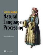
First of all, a typical NER algorithm combines the span identification and the named entity type identification steps into a single, joint task. Second, it approaches this task as a sequence labeling problem: specifically, it goes through the running text word by word and tries to decide whether a word is part of a specific type of a named entity. Figure 11.5 provides the mental model for this process.

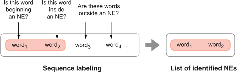
Figure 11.5 Mental model for sequence labeling used to identify NEs in text

In fact, many tasks in NLP are framed as sequence labeling tasks, since language has a clear sequential nature. We have not looked into sequential tasks and sequence labeling in this book before, so let’s discuss this topic now.

11.2 Named-entity recognition as a sequence labeling task

Let’s look closely into what it means for a task to be a sequence labeling task and how this is applied to named-entity recognition. You might have noticed from the examples overviewed in the previous section that ambiguity is present at various levels in language processing, yet whether a word or a phrase is a named entity or not and which type of a named entity it is depends on the context. Not surprisingly, named-entity recognition is addressed using machine-learning algorithms, which are capable of learning useful characteristics of the context. NER is typically addressed with supervised machine-learning algorithms, which means that such algorithms are trained on annotated data. To that end, let’s start with the questions of how the data should be labeled for sequential tasks, such as NER, in a way that the algorithm can benefit from the most.

11.2.1 The basics: BIO scheme

Let’s look again at the example of a sentence with different types of named entities, presented in figure 11.4. We said before that the way the NER algorithm identifies named entities and their types is by considering every word in sequence and deciding whether this word belongs to a named entity of a particular type. For instance, in Apple Inc., the word Apple is at the beginning of a named entity of type ORG and Inc. is at its end. Explicitly annotating the beginning and the end of a named-entity expression and training the algorithm on such annotation helps it capture the information that if a word Apple is classified as beginning a named entity ORG, it is very likely that it will be followed by a word that finishes this named-entity expression.

The labeling scheme that is widely used for NER and similar sequence labeling tasks is called BIO scheme, since it comprises three types of tags: beginning, inside, and outside. We said that the goal of an NER algorithm is to jointly assign to every word its position in a named entity and its type, so in fact this scheme is expanded to accommodate for the type tags too. For instance, there are tags B-PER and I-PER for the words beginning and inside of a named entity of the PER type; similarly, there are B-ORG, I-ORG, B-LOC, I-LOC tags, and so on. O-tag is reserved for all words that are outside of any named entity, and for that reason, it does not have a type extension. Figure 11.6 shows the application of this scheme to the short example “tech giant Apple Inc.”

Figure 11.6 BIO scheme applied to “tech giant Apple Inc.”

In total, there are 2n+1 tags for n named entity types plus a single O-tag: for the 18 NE types from the OntoNotes presented in table 11.1, this amounts to 37 tags in total. BIO scheme has two further extensions that you might encounter in practice: a less fine-grained IO scheme, which distinguishes between the inside and outside tags only, and a more fine-grained BIOES scheme, which also adds an end-of-entity tag for each type and a single-word entity for each type that consists of a single word. Table 11.2 illustrates the application of these annotation schemes to the beginning of our example.

Table 11.2 NER as a sequence labeling task, showing IO, BIO, and BIOES taggings. The notation “...” is used for space reasons for all words that are outside any named entities; they are all marked as O.

This annotation is then used to train the sequential machine-learning algorithm, described in the next section. Before you look into that, try solving exercises 11.3 and 11.4.

11.2.2 What does it mean for a task to be sequential?

Many real-word tasks show sequential nature. As an illustrative example, let’s consider how the temperature of water changes with respect to various possible actions applied to it. Suppose water can stay in one of three states—cold, warm, or hot, as figure 11.7 (left) illustrates. You can apply different actions to it. For example, heat it up or let it cool down. Let’s call a change from one state to another a state transition. Suppose you start heating cold water up and measure water temperature at regular intervals, say, every minute. Most likely you would observe the following sequence of states: cold ® . . . ® cold ® warm ® . . . ® warm ® hot. In other words, to get to the “hot” state, you would first stay in the “cold” state for some time; then you would need to transition through the “warm” state, and finally you would reach the “hot” state. At the same time, it is physically impossible to transition from the “cold” to the “hot” state immediately, bypassing the “warm” state. The reverse is true as well: if you let water cool down, the most likely sequence will be hot ® . . . ® hot ® warm ® . . . ® warm ® cold, but not hot ® cold.

Figure 11.7 Directed graphs visualizing a chain of states (vertices in the graph), transitions (edges), and probabilities associated with these transitions marked on each edge. For example, 0.2 on the edge from “cold” to “warm” in the graph on the left means there is a 0.2 probability of temperature change from the “cold” to the “warm” state. The graph on the left illustrates the water temperature example, and the graph on the right provides an example of transitions between words.

In fact, these types of observations can be formalized and expressed as probabilities. For example, to estimate how probable it is to transition from the “cold” state to the “warm” state, you use your timed measurements and calculate the proportion of times that the temperature transitioned cold ® warm among all the observations made for the “cold” state:

Such probabilities estimated from the data and observations simply reflect how often certain events occur compared to other events and all possible outcomes. Figure 11.7 (left) shows the probabilities on the directed edges. The edges between hot ® cold and cold ® hot are marked with 0.0, reflecting that it is impossible for the temperature to change between “hot” and “cold” directly bypassing the “warm” state. At the same time, you can see that the edges from the state back to itself are assigned with quite high probabilities: P(hot ® hot) = 0.8 means that 80% of the time if water temperature is hot at this particular point in time it will still be hot at the next time step (e.g., in a minute). Similarly, 60% of the time water will be warm at the next time step if it is currently warm, and in 80% of the cases water will still be cold in a minute from now if it is currently cold.

Also note that this scheme describes the set of possibilities fully: suppose water is currently hot. What temperature will it be in a minute? Follow the arrows in figure 11.7 (left) and you will see that with a probability of 0.8 (or in 80% of the cases), it will still be hot and with a probability of 0.2 (i.e., in the other 20%), it will be warm. What if it is currently warm? Then, with a probability of 0.6, it will still be warm in a minute, but there is a 20% chance that it will change to hot and a 20% chance that it will change to cold.

Where do language tasks fit into this? As a matter of fact, language is a highly structured, sequential system. For instance, you can say “Albert Einstein was born in Ulm” or “In Ulm, Albert Einstein was born,” but “Was Ulm Einstein born Albert in” is definitely weird if not nonsensical and can be understood only because we know what each word means and, thus, can still try to make sense of such word salad. At the same time, if you shuffle the words in other expressions like “Ann gave Bob a book,” you might end up not understanding what exactly is being said. In “A Bob book Ann gave,” who did what to whom? This shows that language has a specific structure to it and if this structure is violated, it is hard to make sense of the result.

Figure 11.7 (right) shows a transition system for language, which follows a very similar strategy to the water temperature example from figure 11.7 (left). It shows that if you see a word “a,” the next word may be “book” (“a book”) with a probability of 0.14, “new” (“a new house”) with a 15% chance, or some other word. If you see a word “new,” with a probability of 0.05, it may be followed by another “new” (“a new, new house”), with an 8% chance it may be followed by “a” (“no matter how new a car is, . . .”), in 17% of the cases it will be followed by “book” (“a new book”), and so on. Finally, if the word that you currently see is “book,” it will be followed by “a” (“book a flight”) 13% of the time, by “new” (“book new flights”) 10% of the time, or by some other word (note that in the language example, not all possible transitions are visualized in figure 11.7). Such predictions on the likely sequences of words are behind many NLP applications. For instance, word prediction is used in predictive keyboards, query completion, and so on.

Note that in the examples presented in figure 11.7, the sequential models take into account a single previous state to predict the current state. Technically, such models are called first-order Markov models or Markov chains (for more examples, see section 8.4.1 of Speech and Language Processing by Jurafsky and Martin at https://web.stanford.edu/~jurafsky/slp3/8.pdf). It is also possible to take into account longer history of events. For example, second-order Markov models look into two previous states to predict the current state and so on.

NLP models that do not observe word order and shuffle words freely (as in “A Bob book Ann gave”) are called bag-of-words models. The analogy is that when you put words in a “bag,” their relative order is lost, and they get mixed among themselves like individual items in a bag. A number of NLP tasks use bag-of-words models. The tasks that you worked on before made little if any use of the sequential nature of language. Sometimes the presence of individual words is informative enough for the algorithm to identify a class (e.g., lottery strongly suggests spam, amazing is a strong signal of a positive sentiment, and rugby has a strong association with the sports topic). Yet, as we have noted earlier in this chapter, for NER it might not be enough to just observe a word (is “Apple” a fruit or a company?) or even a combination of words (as in “Amazon River Maps”). More information needs to be extracted from the context and the way the previous words are labeled with NER tags. In the next section, you will look closely into how NER uses sequential information and how sequential information is encoded as features for the algorithm to make its decisions.

11.2.3 Sequential solution for NER

Just like water temperature cannot change from “cold” immediately to “hot” or vice versa without going through the state of being “warm,” and just like there are certain sequential rules to how words are put together in a sentence (with “a new book” being much more likely in English than “a book new”), there are certain sequential rules to be observed in NER. For instance, if a certain word is labeled as beginning a particular type of an entity (e.g., B-GPE for “New” in “New York”), it cannot be directly followed by an NE tag denoting inside of an entity of another type (e.g., I-EVENT cannot be assigned to “York” in “New York” when “New” is already labeled as B-GPE, as I-GPE is the correct tag). In contrast, I-EVENT is applicable to “Year” in “New Year” after “New” being tagged as B-EVENT. To make such decisions, an NER algorithm takes into account the context, the labels assigned to the previous words, and the current word and its properties. Let’s consider two examples with somewhat similar contexts:

Your goal in the NER task is to assign the most likely sequence of tags to each sentence. Ideally, you would like to end up with the following labeling for the sentences: O - O - B-EVENT - I-EVENT for “They celebrated New Year” and O - O - O - B-GPE - I-GPE for “They live in New York.” Figure 11.8 visualizes such “ideal” labeling for “They celebrated New Year” (using an abbreviation EVT for EVENT for space reasons).

Figure 11.8 The “ideal” NE labeling for “They celebrated New Year”. The circles denote states (i.e., NE labels) and the arrows denote transitions from one NE label to the next one. The implausible states for each word are grayed out (e.g., I-EVT for “New”), the implausible transitions are dropped, and the preferred states and transitions are highlighted in bold. Since there are many more labels in the NER scheme, not all of them are included: “...” denotes “any other label” (e.g., B-GPE, I-GPE).

As figure 11.8 shows, it is possible to start a sentence with a word labeled as a beginning of some named entity, such as B-EVENT or B-EVT (as in “Christmas_B-EVT is celebrated on December 25”). However, it is not possible to start a sentence with I-EVT (the tag for inside the EVENT entity), which is why it is grayed out in figure 11.8 and there is no arrow connecting the beginning of the sentence (the START state) to I-EVT. Since the second word, “celebrated,” is a verb, it is unlikely that it belongs to any named entity type; therefore, the most likely tag for it is O. “New” can be at the beginning of event (B-EVT as in “New Year”) or another entity type (e.g., B-GPE as in “New York”), or it can be a word used outside any entity (O). Finally, the only two possible transitions after tag B-EVT are O (if an event is named with a single word, like “Christmas”) or I-EVT. All possible transitions are marked with arrows in figure 11.8; all impossible states are grayed out with the impossible transitions dropped (i.e., no connecting arrows); and the states and transitions highlighted in bold are the preferred ones.

As you can see, there are multiple sources of information that are taken into account here: word position in the sentence matters (tags of the types O and B-ENTITY—outside an entity and beginning an entity, respectively—can apply to the first word in a sentence, but I-ENTITY cannot); word characteristics matter (a verb like “celebrate” is unlikely to be part of any entity); the previous word and tag matter (if the previous tag is B-EVENT, the current tag is either I-EVENT or O); the word shape matters (capital N in “New” makes it a better candidate for being part of an entity, while the most likely tag for “new” is O); and so on.

This is, essentially, how the algorithm tries to assign the correct tag to each word in the sequence. For instance, suppose you have assigned tags O - O - B-EVENT to the sequence “They celebrated New” and your current goal is to assign an NE tag to the word “Year”. The algorithm may consider a whole set of characteristic rules—let’s call them features by analogy with the features used by supervised machine-learning algorithms in other tasks. The features in NER can use any information related to the current NE tag and previous NE tags, current word and the preceding context, and the position of the word in the sentence. Let’s define some feature templates for the features helping the algorithm predict that word₄ in “They celebrated New Year” (i.e., word₄=“Year”) should be assigned with the tag I-EVENT after the previous word “New” is assigned with B-EVENT. It is common to use the notation y_i for the current tag, y_i-1 for the previous one, X for the input, and i for the position, so let’s use this notation in the feature templates:

• f1(y_i-1, y_i, X, i)—If current word is “Year”, return 1; otherwise, return 0.

• f2(y_i-1, y_i, X, i)—If current word is “York”, return 1;otherwise, return 0.

• f3(y_i-1, y_i, X, i)—If previous word is “New”, return 1; otherwise, return 0.

• . . .

• f12(y_i-1, y_i, X, i)—If current word part of speech is noun, return 1; otherwise, return 0.

• f13(y_i-1, y_i, X, i)—If previous word part of speech is adjective, return 1; otherwise, return 0.

• . . .

• f23(y_i-1, y_i, X, i)—If current word is in a gazetteer, return 1; otherwise, return 0.

• . . .

• f34(y_i-1, y_i, X, i)—If current word shape is Xx, return 1; otherwise, return 0.

• . . .

• f45(y_i-1, y_i, X, i)—If current word starts with prefix “Y”, return 1; otherwise, return 0.

• f46(y_i-1, y_i, X, i)—If current word starts with prefix “Ye”, return 1; otherwise, return 0.

• . . .

Note A gazetteer (e.g., www.geonames.org) is a list of place names with millions of entries for locations, including detailed geographical and political information. It is a very useful resource for identification of LOC, GPE, and some other types of named entities.

Note Word shape is determined as follows: capital letters are replaced with X, lowercase letters are replaced with x, numbers are replaced with d, and punctuation marks are preserved; for example, “U.S.A.” can be represented as “X.X.X.” and “11-12p.m.” as “d-dx.x.” This helps capture useful generalizable information.

Feature indexes used in this list are made up, and as you can see, the list of features grows quickly with the examples from the data. When applied to our example, the features will yield the following values:

• f1(y_i-1 = B-EVENT, y_i = I-EVENT, X = “They celebrated New Year”, i = 4) = 1

• f2(y_i-1 = B-EVENT, y_i = I-EVENT, X = “They celebrated New Year”, i = 4) = 0

• f3(y_i-1 = B-EVENT, y_i = I-EVENT, X = “They celebrated New Year”, i = 4) = 1

• . . .

• f12(y_i-1 = B-EVENT, y_i = I-EVENT, X = “They celebrated New Year”, i = 4) = 1

• f13(y_i-1 = B-EVENT, y_i = I-EVENT, X = “They celebrated New Year”, i = 4) = 1

• . . .

• f23(y_i-1 = B-EVENT, y_i = I-EVENT, X = “They celebrated New Year”, i = 4) = 0

• . . .

• f34(y_i-1 = B-EVENT, y_i = I-EVENT, X = “They celebrated New Year”, i = 4) = 1

• . . .

• f45(y_i-1 = B-EVENT, y_i = I-EVENT, X = “They celebrated New Year”, i = 4) = 1

• f46(y_i-1 = B-EVENT, y_i = I-EVENT, X = “They celebrated New Year”, i = 4) = 1

It should be noted that no single feature is capable of correctly identifying an NE tag in all cases; moreover, some features may be more informative than others. What the algorithm does in practice is it weighs the contribution from each feature according to its informativeness and then it combines the values from all features, ranging from feature k = 1 to feature k = K (where k is just an index), by summing the individual contributions as follows:

Equation 11.1 Sum over all features from feature with index k = 1 to k = K over the feature values f_k (equal to either 0 or 1) multiplied with respective weights w_k.

For example, if w1 for f1 is 0.4, w2 for f2 is 0.4, and w3 for f3 is 0.2, then the sum over these three features using the values for “They celebrated New Year” from above is

Result = w1 × f1 + w2 × f2 + w3 × f3 = 0.4 × 1 + 0.4 × 0 + 0.2 × 1 = 0.6

The appropriate weights in this equation are learned from labeled data as is normally done for supervised machine-learning algorithms. As was pointed out earlier, the ultimate goal of the algorithm is to assign the correct tags to all words in the sequence, so the expression is actually applied to each word in sequence, from i = 1 (i.e., the first word in the sentence) to i = n (the last word); that is,

Equation 11.2 Apply the estimation from Equation 11.1 to each word in the sequence and sum the results over all words from i = 1 to i = n.

Specifically, this means that the algorithm is not only concerned with the correct assignment of the tag I-EVENT to “Year” in “They celebrated New Year”, but also with the correct assignment of the whole sequence of tags O - O - B-EVENT - I-EVENT to “They celebrated New Year”. However, originally, the algorithm knows nothing about the correct tag for “They” and the correct tag for “celebrated” following “They”, and so on. Since originally the algorithm doesn’t know about the correct tags for the previous words, it actually considers all possible tags for the first word, then all possible tags for the second word, and so on. In other words, for the first word, it considers whether “They” can be tagged as B-EVENT, I-EVENT, B-GPE, I-GPE, . . . , O, as figure 11.8 demonstrated earlier; then for each tag applied to “They”, the algorithm moves on and considers whether “celebrated” can be tagged as B-EVENT, I-EVENT, B-GPE, I-GPE, . . . , O; and so on. In the end, the result you are interested in is the sequence of all NE tags for all words that is most probable; that is,

Equation 11.3 Use the estimation from Equation 11.2 and return the sequence of tags, which results in the maximum value.

The formula in Equation 11.3 is exactly the same as the one in Equation 11.2, with just one modification: argmax means that you are looking for the sequence that results in the highest probability estimated by the rest of the formula; Y stands for the whole sequence of tags for all words in the input sentence; and the fancy font Y denotes the full set of possible combinations of tags. Recall the three BIO-style schemes introduced earlier in this chapter: the most coarse-grained IO scheme has 19 tags, which means that the total number of possible tag combinations for the sentence “They celebrated New Year”, consisting of 4 words, is 19⁴=130,321; the middle-range BIO scheme contains 37 distinct tags and results in 37⁴=1,874,161 possible combinations; and finally, the most fine-grained BIOES scheme results in 73⁴=28,398,241 possible tag combinations for a sentence consisting of 4 words. Note that a sentence consisting of 4 words is a relatively short sentence, yet the brute-force algorithm (i.e., the one that simply iterates through each possible combination at each step) rapidly becomes highly inefficient. After all, some tag combinations (like O ® I-EVENT) are impossible, so there is no point in wasting effort on even considering them. In practice, instead of a brute-force algorithm, more efficient algorithms based on dynamic programming are used (the algorithm that is widely used for language-related sequence labeling tasks is the Viterbi algorithm; you can find more details in section 8.4.5 of Speech and Language Processing by Jurafsky and Martin at https://web.stanford.edu/~jurafsky/slp3/8.pdf).

Instead of exhaustively considering all possible combinations, at each step a dynamic programming algorithm calculates the probability of all possible solutions given only the best, most optimal solution for the previous step. The algorithm then calculates the best move at the current point and stores it as the current best solution. When it moves to the next step, it again considers only this best solution rather than all possible solutions, thus considerably reducing the number of overall possibilities to only the most promising ones. Figure 11.9 demonstrates the intuition behind dynamic estimation of the best NE tag that should be selected for “Year” given that the optimal solution O - O - B-EVENT is found for “They celebrated New”.

Figure 11.9 A dynamic programming algorithm solves the following task: if the best (most likely) tag sequence so far is O - O - B-ENT, what is the most likely tag for “Year” at this point?

This, in a nutshell, is how a sequence labeling algorithm solves the task of tag assignment. As was highlighted before, NER is not the only task that demonstrates sequential effects, and a number of other tasks in NLP are solved this way. One task that you have encountered before in this book, which is also a sequence labeling task and which, under the hood, is solved in a similar manner, is POS tagging. You looked into this task in chapter 4 and used POS tags as features in NLP applications in later chapters. The approach to sequence labeling outlined in this section is used by machine-learning algorithms, most notably, conditional random fields (for further examples, see section 8.5 of Speech and Language Processing by Jurafsky and Martin at https://web.stanford.edu/~jurafsky/slp3/8.pdf), although you don’t need to implement your own NER to be able to benefit from the results of this step in the NLP pipeline. For instance, spaCy has an NER implementation that you are going to rely on to solve the task set out in the scenario for this chapter. The next section delves into implementation details.

11.3 Practical applications of NER

Let’s remind ourselves of the scenario for this chapter. It is widely known that certain events influence the trends of stock price movements. Specifically, you can extract relevant facts from the news and then use these facts to predict company stock prices. Suppose you have access to a large collection of news; now your task is to extract the relevant events and facts that can be linked to the stock market in the downstream (stock market price prediction) application. How will you do that?

This means that you have access to a collection of news texts, and among other preprocessing steps, you apply NER. Then you can focus only on the texts and sentences that are relevant for your task. For instance, if you are interested in the recent events, in which a particular company (e.g., “Apple”) participated, you can easily identify such texts, sentences, and contexts. Figure 11.10 shows a flow diagram for this process.

Figure 11.10 Practical application of NER in downstream tasks (e.g., in further information extraction)

11.3.1 Data loading and exploration

There are multiple ways in which you can get access to news articles, such as extracting the up-to-date news articles from the news portals in real time. This, of course, would be a reasonable approach if you wanted to build an application that can predict outcomes for the current events. For the sake of the exercise in this chapter, however, we are going to use the data that has already been extracted from a range of news portals. The dataset called “All the news” is hosted on the Kaggle website (www.kaggle.com/snapcrack/all-the-news). The dataset consists of 143,000 articles scraped from 15 news websites, including the New York Times, CNN, Business Insider, Washington Post, and so on. The dataset is quite big and is split into three comma-separated values (CSV) files. In the examples in this chapter, you are going to be working with the file called articles1.csv, but you are free to use other files in your own experiments.

Many datasets available via Kaggle and similar platforms are stored in the .csv format. This basically means that the data is stored as a big spreadsheet file, where information is split between different rows and columns. For instance, in articles1.csv, each row represents a single news article, described with a set of columns containing information on its title, author, the source website, the date of publication, its full content, and so on. The separator used to define the boundary between the information belonging to different data fields in .csv files is a comma. It’s time now to familiarize yourselves with pandas, a useful data-preprocessing toolkit that helps you work with files in such formats as .csv and easily extract information from them.

Let’s use this toolkit to extract the information from the input file as listing 11.2 shows. In this code, you import pandas once you’ve installed it. Since the dataset is split into multiple files, you need to provide the path location for the files, and then you can open a particular file using pandas read_csv functionality. The result is stored in a DataFrame df.

Listing 11.2 Code to extract the data from the input file using pandas

import pandas as pd                         ❶
 
path = "all-the-news/"                      ❷
df = pd.read_csv(path + "articles1.csv")    ❸

❶ Import pandas once you’ve installed it.

❷ Provide the path location for the files.

❸ Open the file using pandas read_csv functionality; the result is stored in a DataFrame df.

The code from listing 11.2 reads the contents of the .csv file, using a comma as a delimiter to identify which information field (column) a particular string of text in the row belongs to. The result is called a DataFrame, a labeled data structure with columns of potentially different types (e.g., they can contain textual as well as numerical information). Pandas provides you with extensive functionality and allows you to investigate the contents of the DataFrame from various perspectives. You can learn more about this tool’s functionality from the documentation. The most useful functions at this point in your application are df.shape and df.head(). The function df.shape prints out the dimensionality of the data structure. For articles1.csv, it is (50000, 10)—that is, 50,000 rows representing individual news articles to 10 columns containing various information on these articles, from titles, to publication dates, to the full article content. The function df.head() prints out the first five rows from your DataFrame. Both these functions serve as useful sanity checks. It is always a good idea to check what the data you are working with contains. Here is what df.head() returns for the DataFrame initialized in listing 11.2:

You can now explore the data in your DataFrame in more detail. For example, since the data from 15 news sources is split between several .csv files, let’s find out which news sources are covered by the current DataFrame. Listing 11.3 shows how to do that. Specifically, you need to extract the information from a particular column (here, "publication") and apply unique() function to convert the result into a set.

Listing 11.3 Code to extract the information on the news sources only

sources = df["publication"].unique()    ❶
print(sources)

❶ Extract the information from the “publication” column and convert the result into a set.

As you can see, pandas provides you with an easy way to extract and explore the information you need at this point. With just one line of code, you extract the contents of the column entitled "publication" in the DataFrame (this column indicates the news source for each article), and then apply the function unique() that converts the list into a set of unique values. Here is the output that this code produces:

['New York Times' 'Breitbart' 'CNN' 'Business Insider' 'Atlantic']

Since the DataFrame contains as many as 50,000 articles, for the sake of this application, let’s focus on some articles only. We will extract the text (content) of the first 1,000 articles published in the New York Times. Listing 11.4 shows how to do that. First, you define a condition—the publication source should be "New York Times". Then you select the content from all articles that satisfy this condition (i.e., df.loc[condition, :]), and from these, you extract only the first 1,000 for simplicity. In the end, you can check the dimensionality of the extracted data structure using df.shape as before.

Listing 11.4 Code to extract the content of articles from a specific source

condition = df["publication"].isin(["New York Times"])    ❶
content_df = df.loc[condition, :]["content"][:1000]       ❷
content_df.shape                                          ❸

❶ Define a condition for the publication source to be “New York Times”.

❷ Select the content from all articles that satisfy this condition and only extract the first 1,000 of them.

❸ Check the dimensionality of the extracted data structure using df.shape as before.

The code prints out (1000,), confirming that you extracted 1,000 articles from the New York Times. The new data structure, content_df, is simply an array of 1,000 news texts. You can further check the contents of these articles using the functions mentioned before; for example, content_df.head() will show the following content from the first five articles:

11.3.2 Named entity types exploration with spaCy

Now that the data is loaded, let’s explore what entity types it contains. For that, you can rely on the NER functionality from spaCy (for more examples and more information, check spaCy’s documentation at https://spacy.io/usage/linguistic-features#named-entities). Recall that you used it in an earlier exercise in listing 11.1.

Let’s start by iterating through the news articles, collecting all named entities identified in texts and storing the number of occurrences in a Python dictionary, as figure 11.11 illustrates.

Figure 11.11 Extract all named entities from news articles and store them in a Python dictionary.

Listing 11.5 shows how to populate a dictionary with the named entities extracted from all news articles in content_df. First, you import spaCy and load a language model (here, medium size). Next, you define the collect_entities function, which extracts named entities from all news articles and stores the statistics on them in the Python dictionary named_entities. Within this function, you process each news article with spaCy’s NLP pipeline and store the result in the processed_docs list for future use. Specifically, for each entity, you extract the text with ent.text (e.g., Apple) and store it as entity_text. In addition, you identify the type of the entity with ent.label_ (e.g., ORG) and store it as entity_type. Then, for each entity type (e.g., ORG), you extract the list of entities and their counts (e.g., [Facebook: 175, Apple Inc.: 63, ...] currently stored in current_ents. After that, you update the counts in current_ents, incrementing the count for the entity stored as entity_text, and finally, you return the named_entities dictionary and the processed_docs list.

Listing 11.5 Code to populate a dictionary with NEs extracted from news articles

import spacy
nlp = spacy.load("en_core_web_md")                                ❶
 
def collect_entites(data_frame):                                  ❷
    named_entities = {}
    processed_docs = []
 
    for item in data_frame:
        doc = nlp(item)
        processed_docs.append(doc)                                ❸
 
        for ent in doc.ents:
            entity_text = ent.text                                ❹
            entity_type = str(ent.label_)                         ❺
            current_ents = {}                                     ❻
            if entity_type in named_entities.keys():
                current_ents = named_entities.get(entity_type)
            current_ents[entity_text] = current_ents.get(entity_text, 0) + 1
            named_entities[entity_type] = current_ents            ❼
    return named_entities, processed_docs
 
named_entities, processed_docs = collect_entites(content_df)      ❽

❶ Import spaCy and load a language model (here, medium-size).

❷ Define the collect_entities function to extract named entities and store the statistics on them.

❸ Process each news article with spaCy’s NLP pipeline and store the result in the processed_docs list.

❹ For each entity, extract the text with ent.text (e.g., Apple) and store it as entity_text.

❺ Identify the type of the entity with ent.label_ (e.g., ORG) and store it as entity_type.

❻ For each entity type, extract the list of currently stored entities with their counts.

❼ Update the counts in current_ents, incrementing the count for the entity stored as entity_text.

❽ Return the named_entities dictionary and the processed_docs list.

To inspect the results, let’s print out the contents of the named_entities dictionary, as listing 11.6 suggests. In this code, you print out the type of a named entity (e.g., ORG) and for each type, you extract all entities assigned with this type in the dictionary (e.g., [Facebook: 175, Apple Inc.: 63, ...]). Then you sort the entries by their frequency in descending order. For space reasons, this code suggests that you only print out the most frequent n ones (e.g., 10 here) of them. Additionally, it would be most informative to only look into entities that occur more than once. In the end, you print out the named entities and frequency counts.

Listing 11.6 Code to print out the named entities dictionary

def print_out(named_entities):
    for key in named_entities.keys():                                  ❶
        print(key)
        entities = named_entities.get(key)                             ❷
        sorted_keys = sorted(entities, key=entities.get, reverse=True)
        for item in sorted_keys[:10]:                                  ❸
            if (entities.get(item)>1):                                 ❹
                print("   " + item + ": " + str(entities.get(item)))   ❺
 
print_out(named_entities)

❶ Print out the type of a named entity (e.g., ORG).

❷ Extract all entities of a particular type from the dictionary.

❸ Sort the entries by their frequency in descending order and print out the most frequent n ones.

❹ It would be most informative to only look into entities that occur more than once.

❺ Print out the named entity and its frequency.

This code prints out all 18 named entity types with up to 10 most frequent named entities for each type. The full list is, of course, much longer, with many entities occurring in the data only a few times (that is why we limit the output here to the most frequent items only). Here is the output printed out for the GPE type:

GPE
   the United States: 1148
   Russia: 526
   China: 515
   Washington: 498
   New York: 365
   America: 359
   Iran: 294
   Mexico: 265
   Britain: 236
   California: 203

Note These results are obtained with the versions of tools specified in the installation instructions. As before, if you are using different versions of tools or a model different from en_core_web_md, it is possible that the precise numbers that you are getting are slightly different and you shouldn’t be alarmed by this difference in the results.

Perhaps not surprisingly, the most frequent geopolitical entity mentioned in the New York Times articles is the United States. It is mentioned 1,148 times in total; in fact, this can be combined with the counts for other expressions used for the same entity (e.g., America and the like). It is followed by Russia (526 times) and China (515). As you can see, there is a lot of information contained in this dictionary.

Another way in which you can explore the statistics on various NE types is to aggregate the counts on the types and print out the number of unique entries (e.g., Apple and Facebook would be counted as two separate named entities under the ORG type), as well as the total number of occurrences of each type (e.g., 175 counts for Facebook and 63 for Apple would result in the total number of 238 occurrences of the type ORG). Listing 11.7 shows how to do that. It suggests that you print out information on the entity type (e.g., ORG), the number of unique entries belonging to a particular type (e.g., Apple and Facebook would contribute as two different entries for ORG), and the total number of occurrences of the entities of that particular type. To do that, you extract and aggregate the statistics for each NE type, and in the end, you print out the results in a tabulated format, with each row storing the statistics on a separate NE type.

Listing 11.7 Code to aggregate the counts on all named entity types

rows = []
rows.append(["Type:", "Entries:", "Total:"])       ❶
for ent_type in named_entities.keys():
    rows.append([ent_type, str(len(named_entities.get(ent_type))), 
                 str(sum(named_entities.get(
                     ent_type).values()))])        ❷
 
columns = zip(*rows)
column_widths = [max(len(item) for item in col) for col in columns]
for row in rows:
    print(''.join(' {:{width}} '.format(row[i], width=column_widths[i]) 
                  for i in range(0, len(row))))    ❸

❶ Print out the entity type, the number of unique entries, and the total number of entities occurrences.

❷ Extract and aggregate the statistics for each NE type.

❸ Print out the results, with each row storing the statistics on a separate NE type.

This code prints out the results shown in table 11.3.

Table 11.3 Aggregated statistics on the named entities from the news articles dataset—the NE types, the number of unique entries, and the total number of occurrences.

As this table shows, the most frequently used named entities in the news articles are entities of the following types: PERSON, GPE, ORG, and DATE. This is, perhaps, not very surprising. After all, most often news reports on the events that are related to people (PERSON), companies (ORG), countries (GPE), and usually news articles include references to specific dates. At the same time, the least frequently used entities are the ones of the type LANGUAGE: there are only 12 unique languages mentioned in this news articles dataset, and in total they are mentioned 85 times. Among the most frequently mentioned are English (48 times), Arabic (8), and Spanish (7). You may also note that the ORDINAL type has only 68 unique entries: it is, naturally, a very compact list of items including entries like first, second, third, and so on.

11.3.3 Information extraction revisited

Now that you have explored the data, you can look more closely into the information that the articles contain on specific entities of interest. Consider the scenario again: your task is to build an information extraction application focused on companies and the news that reports on these companies. The dataset at hand, according to table 11.4, contains information on as many as 4,892 companies. Of course, not all of them will be of interest to you, so it would make sense to select a few and extract information on them.

Chapter 4 looked into the information extraction task, which was concerned with the extraction of relevant facts (e.g., actions in which certain personalities of interest are involved). Let’s revisit this task here, making the necessary modifications. Specifically, the following ones:

• Let’s extract actions together with their participants but focus on participants of a particular type, such as companies (ORG) or a specific company (Apple). For that, you will work with a subset of sentences that contain the entity of interest.

• Let’s extract the contexts in which an entity of interest (e.g., Apple) is one of the main participants (e.g., “Apple sued Qualcomm” or “Russia required Apple to . . .”). For that, you will use the linguistic information from spaCy’s NLP pipeline, focusing on the cases where the entity is the subject (the main participant of the main action as Apple is in “Apple sued Qualcomm”) or the object (the second participant of the main action as Apple is in “Russia required Apple to . . .”). This information can be extracted from the spaCy’s parser output using nsubj and dobj relations, respectively.

• Oftentimes the second participant of the action is linked to the main verb via a preposition. For instance, compare “Russia required Apple” to “The New York Times wrote about Apple”. In the first case, Apple is the direct object of the main verb required, and in the second case, it is an indirect object of the main verb wrote. Let’s make sure that both cases are covered by our information extraction algorithm.

• Finally, as observed in the earlier examples, named entities may consist of a single word (Apple) or of several words (Apple Inc.). To that end, let’s make sure the code applies to both cases.

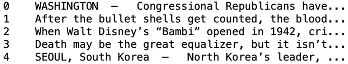
Recall that spaCy’s NLP pipeline processes sentences (or full documents) and returns a data structure, which contains all sorts of information on the words in the sentence (text), including the information about the word’s type (part of speech, such as verb, noun, etc.), its named entity type, and its role in the sentence (e.g., main verb—ROOT, main action’s participant—nsubj). Figure 11.12 provides a reminder.

Figure 11.12 A reminder on the information provided on the word tokens by spaCy pipeline

In addition, each word has a unique index that is linked to its position in the sentence. If a named entity consists of multiple words, some of them may be marked with the nsubj or dobj relations (i.e., relevant relations in your application), but your goal is to extract not only the word marked as nsubj or dobj but also the whole named entity, which plays this role. To do that, the best way is to match the named entities to their roles in the sentence via the indexes assigned to the named entities in the sentence. Figure 11.13 illustrates this process.

Figure 11.13 The aim of the extraction algorithm is to identify whether the named entity of interest is one of the participants in the main action; that is, a subject or an object of the main verb. In a multiword NE, only one word will be marked with the relevant role (e.g., nsubj here), but the code needs to return the whole NE.

Specifically, figure 11.13 looks into the following example: suppose your named entity of interest is a multiword expression “The New York Times” and the full sentence is “The New York Times wrote about Apple”. Your goal is to identify whether “The New York Times” is one of the participants of the main action (wrote) in this sentence; in other words, if it is the subject (the entity that performs the action) or an object (an entity to which the action applies). Indeed, “The New York Times” as a whole is the subject; it is the entity that performed the action of writing. However, since linguistic analysis applies to individual words rather than whole expressions, technically only the word “Times” is directly dependent on the main verb “wrote”; this is shown through the chain of relations in figure 11.13. How can you extract the whole expression “The New York Times”?

To do that, you first identify the indexes of the words covered by this expression in the sentence. For “The New York Times”, these are [0, 1, 2, 3], as the left part of figure 11.13 shows. Next, you check if a word with any of these indexes plays a role of the subject or an object in the sentence. Indeed, the word that is the subject in the sentence has the index of 3 (as is shown on the right-hand side of figure 11.13). Therefore, you can return the whole named entity “The New York Times” as the subject of the main action in the sentence.

The first step concerned with the identification of the indexes of the words contained in the named entity in question is solved with the code from listing 11.8. In this code, you define extract_span function, which takes as input a sentence and the entity of interest. It then populates the list of indexes with the indexes of the words included in the NE and returns the indexes list as an output.

Listing 11.8 Code to extract the indexes of the words covered by the NE

def extract_span(sent, entity):      ❶
    indexes = []
    for ent in sent.ents:
        if ent.text==entity:
            for i in range(int(ent.start), int(ent.end)):
                indexes.append(i)    ❷
    return indexes                   ❸

❶ Define the extract_span function, which takes as input a sentence and the entity of interest.

❷ Populate the list of indexes with the indexes of the words included in the NE.

❸ Return the indexes list as an output.

This code returns [0, 1, 2, 3] for extract_span ("The New York Times wrote about Apple", "The New York Times").

The second half of the task, the one concerned with the identification of whether a named entity in question plays the role of one of the participants in the main action, is solved with the code from listing 11.9. This code may look familiar to you. It is a modification of a solution that was applied to extract information in chapter 4. In this code, you define the extract_information function, which takes a sentence, the entity of interest, and the list of the indexes of all the words covered by this entity as an input. Then you initialize the list of actions and an action with two participants. Next, you identify the main verb expressing the main action in the sentence and initialize the indexes for the subject and the object related to this main verb. The main verb itself is stored in the action variable; you can find the subject that is related to the main verb via the nsubj relation and store it as participant1 and its index as subj_ind. If there is a preposition attached to the verb (e.g., “write about”), then you need to search for the indirect object as the second participant. If such an object is a noun or a proper noun, you store it as participant2 and its index as obj_ind. If at this point both participants of the main action have been identified and their indexes are included in the indexes of the words covered by the entity, you add the action with two participants to the list of actions. Otherwise, if there is no preposition attached to the verb, participant2 is a direct object of the main verb, which can be identified via the dobj relation (e.g., “X bought Y”). In this case, you apply the same strategy as earlier, adding the action with two participants to the list of actions. In the end, if the final list of actions is not empty, you print out the sentence and all actions together with the participants.

Listing 11.9 Code to extract information about the main participants of the action

def extract_information(sent, entity, indexes):                                   ❶
    actions = []
    action = ""
    participant1 = ""
    participant2 = ""                                                             ❷
        
    for token in sent:
        if token.pos_=="VERB" and token.dep_=="ROOT":                             ❸
            subj_ind = -1
            obj_ind = -1                                                          ❹
            action = token.text                                                   ❺
            children = [child for child in token.children]   
            for child1 in children:
                if child1.dep_=="nsubj":
                    participant1 = child1.text
                    subj_ind = int(child1.i)                                      ❻
                if child1.dep_=="prep":
                    participant2 = ""
                    child1_children = [child for child in child1.children]
                    for child2 in child1_children:
                        if child2.pos_ == "NOUN" or child2.pos_ == "PROPN":
                            participant2 = child2.text
                            obj_ind = int(child2.i)                               ❼
                    if not participant2=="":
                        if subj_ind in indexes:
                            actions.append(entity + " "
                                           + action + " " + child1.text
                                           + " " + participant2)
                        elif obj_ind in indexes:
                            actions.append(participant1 + " " + action + 
                            " " + child1.text + 
                            " " + entity)                                         ❽
                if child1.dep_=="dobj" and (child1.pos_ == "NOUN"
                                            or child1.pos_ == "PROPN"):
                    participant2 = child1.text
                    obj_ind = int(child1.i)
                    if subj_ind in indexes:
                        actions.append(entity + " " + action + " " + participant2)
                    elif obj_ind in indexes:
                        actions.append(participant1 + " " + action + " " + entity)❾
                    
    if not len(actions)==0:
        print (f"
Sentence = {sent}")
        for item in actions:
            print(item)                                                           ❿

❶ Define the extract_information function.

❷ Initialize the list of actions and an action with two participants.

❸ Identify the main verb expressing the main action in the sentence.

❹ Initialize the indexes for the subject and the object related to the main verb.

❺ Store the main verb itself in the action variable.

❻ Find the subject via the nsubj relation and store it as participant1 and its index as subj_ind.

❼ Search for the indirect object as the second participant and store it as participant2 and its index as obj_ind.

❽ If both participants of the action are identified, add the action with two participants to the list of actions.

❾ If there is no preposition attached to the verb, find a direct object of the main verb via the dobj relation.

❿ If the final list of actions is not empty, print out the sentence and all actions together with the participants.

Now let’s apply this code to your texts extracted from the news articles. Note, however, that the code in listing 11.9 applies to the sentence level, since it relies on the information extracted from the parser (which applies to each sentence rather than the whole text). In addition, if you are only interested in a particular entity, it doesn’t make sense to waste the algorithm’s efforts on the texts and sentences that don’t mention this entity at all. To this end, let’s first extract all sentences that mention the entity in question from processed_docs and then apply the extract_information method to extract all tuples (participant1 + action + participant2) from the sentences, where either participant1 or participant2 is the entity you are interested in.

Listing 11.10 shows how to do that. In this code, you define the entity_detector function that takes processed_docs, the entity of interest, and its type as input. If a sentence contains the input entity (e.g., Apple) of the specified type (e.g., ORG) among its named entities, you add this sentence to the output_sentences. Using this function, you find all sentences for a specific entity and print out the number of such sentences found. In the end, you apply extract_span and extract_information functions from the previous code listings to extract the information on the entity of interest from the set of sentences containing this entity.

Listing 11.10 Code to extract information on the specific entity

def entity_detector(processed_docs, entity, ent_type):      ❶
 
    output_sentences = []
    for doc in processed_docs:
        for sent in doc.sents:
            if entity in [ent.text for ent in sent.ents if 
                          ent.label_==ent_type]:
                output_sentences.append(sent)              ❷
    return output_sentences   
 
entity = "Apple"
ent_sentences = entity_detector(processed_docs, entity, "ORG")
print(len(ent_sentences))                                  ❸
 
for sent in ent_sentences:
    indexes = extract_span(sent, entity)
    extract_information(sent, entity, indexes)             ❹

❶ Define the entity_detector function that takes processed_docs, the entity of interest, and its type as input.

❷ Only consider sentences that contain the input entity of the specified type among its named entities.

❸ Find all sentences for a specific entity and print out the number of such sentences found.

❹ Apply extract_span and extract_information functions from the previous code listings.

This code uses “Apple” as the entity of interest and specifically looks for sentences, in which the company (ORG) Apple is mentioned. As the printout message shows, there are 59 such sentences. Not all sentences among these 59 sentences mention Apple as a subject or object of the main action, but the last line of code returns a number of such sentences with the tuples summarizing the main content:

Sentence = Apple has previously removed other, less prominent media apps from its China store.
Apple removed apps
 
Sentence = Russia required Apple and Google to remove the LinkedIn app from their local stores.
Russia required Apple
 
Sentence = On Friday, Apple, its longtime partner, sued Qualcomm over what it said was $1 billion in withheld rebates.
Apple sued Qualcomm

The main content of the sentences is concisely summarized by the tuples consisting of the main action and its two participants, so if you were interested in extracting only the sentences that have such informative content and that directly answer questions “What did Apple do to X?” or “What did Y do to Apple?” you could use the code from listing 11.10.

11.3.4 Named entities visualization

One of the most useful ways to explore named entities contained in text and to extract relevant information is to visualize the results of NER. For instance, the code from listing 11.10 allows you to extract the contexts in which a named entity of interest is one of the main participants, but what about all the other contexts? Among those missed by the algorithm applied in listing 11.10 might be sentences with interesting and relevant content. To that end, let’s revisit extraction of sentences containing the entity in question and explore visualization to highlight the use of the entity alongside other relevant entities.

Listing 11.11 uses spaCy’s visualization tool, displaCy, which allows you to highlight entities of different types in the selected set of sentences using distinct colors for each type (see documentation on displaCy here: https://spacy.io/usage/visualizers). Specifically, after displacy is imported, you define the visualize function that takes processed_docs, an entity of interest, and its type as input, identifies the sentences that contain the entity in question, and visualizes the context. You can test this code by applying it to any selected example.

Listing 11.11 Code to visualize named entities of various types in their contexts of use

from spacy import displacy                              ❶
 
def visualize(processed_docs, entity, ent_type):        ❷
    for doc in processed_docs:
        for sent in doc.sents:
            if entity in [ent.text for ent in sent.ents 
                          if ent.label_==ent_type]:
                displacy.render(sent, style="ent")      ❸
 
visualize(processed_docs, "Apple", "ORG")               ❹

❶ Import displacy.

❷ Define visualize function that takes processed_docs, an entity of interest, and its type as input.

❸ Identify the sentences that contain the entity in question and visualize the context.

❹ Apply this code to a selected example.

This code displays all sentences, in which the company (ORG) Apple is mentioned. Other entities are highlighted with distinct colors. Figure 11.14 shows a small portion of the output.

Figure 11.14 Contexts, in which the company (ORG) Apple is mentioned alongside other named entities. Entities of different types are highlighted using distinct colors.

Finally, you might be interested specifically in the contexts in which the company Apple is mentioned alongside other companies. Let’s filter out all other information and highlight only named entities of the same type as the entity in question (i.e., all ORG NEs in this case). Listing 11.12 shows how to do that. Here, you define the count_ents function that counts the number of entities of a certain type in a sentence. With an updated entity_detector_custom function, you extract only the sentences that mention the input entity of a specified type as well as at least one other entity of the same type. You can print out the number of sentences identified this way as a sanity check. Then you define the visualize_type function that applies visualization to the entities of a predefined type only. spaCy allows you to customize the colors for visualization and to apply gradient (you can choose other colors from https://htmlcolorcodes.com/color-chart/), and using this customized color scheme, you can finally visualize the results.

Listing 11.12 Code to visualize named entities of a specific type only

def count_ents(sent, ent_type):                                  ❶
    return len([ent.text for ent in sent.ents if ent.label_==ent_type])   
 
def entity_detector_custom(processed_docs, entity, ent_type):
    output_sentences = []
    for doc in processed_docs:
        for sent in doc.sents:
            if entity in [ent.text for ent in sent.ents 
                          if ent.label_==ent_type and 
                          count_ents(sent, ent_type)>1]:
                output_sentences.append(sent)
    return output_sentences                                      ❷
 
output_sentences = entity_detector_custom(processed_docs, "Apple", "ORG")
print(len(output_sentences))                                     ❸
 
def visualize_type(sents, entity, ent_type):                     ❹
    colors = {"ORG": 
              "linear-gradient(90deg, #64B5F6, #E0F7FA)"}        ❺
    options = {"ents": ["ORG"], "colors": colors}
    for sent in sents:
        displacy.render(sent, style="ent", options=options)      ❻
                
visualize_type(processed_docs, "Apple", "ORG")

❶ Define the count_ents function that counts the number of entities of a certain type in a sentence.

❷ Extract sentences that mention entity of a specified type as well as at least one other entity of the same type.

❸ Print out the number of sentences identified this way.

❹ Define the visualize_type function that applies visualization to the entities of a predefined type only.

❺ spaCy allows you to customize the colors for visualization and to apply gradient.

❻ Visualize the results using the customized color scheme.

Figure 11.15 shows some of the output of this code.

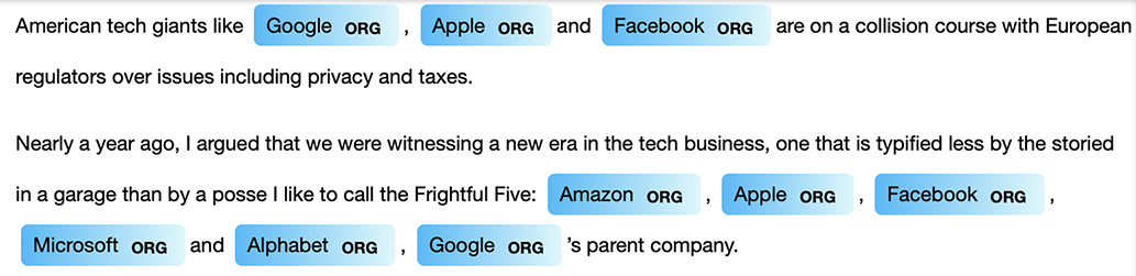
Figure 11.15 Visualization of the company names in contexts mentioning the selected company of interest (Apple) using customized color scheme

Congratulations! With the code from this chapter, you can now extract from a collection of news articles all relevant events and facts summarizing the actions undertaken by the participants of interest, such as specific companies. These events can be further used in downstream tasks. For example, if you also harvest data on stock price movements, you can link the events extracted from the news to the changes in the stock prices immediately following such events, which will help you to predict how the stock price may change in view of similar events in the future.

Summary

• Named-entity recognition (NER) is one of the core NLP tasks; however, when the main goal of the application you are developing is not concerned with improving the core NLP task itself but rather relies on the output from the core NLP technology, this is called a downstream task. The tasks that benefit from NER include information extraction, question answering, and the like.

• Named entities are real-world objects (people, locations, organizations, etc.) that can be referred to with a proper name, and named-entity recognition is concerned with identification of the full span of such entities (as entities may consist of a single word like Apple or of multiple words like Albert Einstein) and the type of the expression.

• The four most widely used types include person, location, organization, and geopolitical entity, although other types like time references and monetary units are also typically added. Moreover, it is also possible to train a customized NER algorithm for a specific domain. For instance, in biomedical texts, gene and protein names represent named entities.

• NER is a challenging task. The major challenges are concerned with the identification of the full span of the expression (e.g., Amazon versus Amazon River) and the type (e.g., Washington may be an entity of up to 4 different types depending on the context). The span and type identification are the tasks that in NER are typically solved jointly.

• The set of named entities often used in practice is derived from the OntoNotes, and it contains 18 distinct NE types. The annotation scheme used to label NEs in data is called a BIO scheme (with a more coarse-grained variant being the IO, and the more fine-grained one being the BIOES scheme). This scheme explicitly annotates each word as beginning an NE, being inside of an NE, or being outside of an NE.

• The NER task is typically framed as a sequence labeling task, and it is commonly addressed using a feature-based approach. NER is not the only NLP task that is solved using sequence labeling, since language shows strong sequential effects. Part-of-speech tagging overviewed in chapter 4 is another example of a sequential task.

• You can apply spaCy in practice to extract named entities of interest and facts related to these entities from a collection of news articles.

• A very popular format in data science is CSV, which uses a comma as a delimiter. An easy-to-use open source data analysis and manipulation tool for Python practitioners that helps you work with such files is pandas.

• Finally, you can explore the results of NER visually, using the displaCy tool and color-coding entities of different types with its help.

Conclusion

This chapter concludes the introductory book on natural language processing. You have covered a lot of ground since you first opened this book. Let’s briefly summarize what you have learned:

• The first couple of chapters provided you with a mild introduction into the field of NLP, using examples of applications in everyday life that, under the hood, rely on NLP technology. You looked into some of these applications in more detail and learned about the core tasks and techniques.

• The earlier chapters of this book focused on the introduction of the fundamental NLP concepts and methods. You learned about tokenization, stemming and lemmatization, part-of-speech tagging and dependency parsing, among other things. To put these concepts and techniques in context, each of them was introduced as part of a more focused, practical NLP task. For instance, the earlier chapters focused on the development of such applications as information search and information extraction.

• This book has taken a practical approach to learning from early on. Indeed, there is no better way to acquire new knowledge and skills than to put them in practice straightaway. Apart from the information search and the information extraction applications, you have also built your own spam filter, authorship attribution algorithm, sentiment analyzer, and topic classifier.

• Machine-learning techniques play an important role in NLP these days and are widely used across various NLP tasks. This book has introduced you to a range of ML approaches covering supervised, unsupervised, and sequence-labeling frameworks.

• Finally, this book has introduced good project development practices as each application followed the crucial steps in a data science project: from data exploration to preparation and preprocessing, to algorithm development, to evaluation.

The field of NLP is one of the most popular and quickly developing fields in artificial intelligence and data science. The primary goal of this book has been to introduce you to this exciting and highly innovative field and equip you with the core knowledge and skills that would allow you to further explore the vast number of opportunities in this area. I sincerely hope that you will continue your journey. Here are some further pointers, where you can get ideas for your future NLP projects:

• State-of-the-art NLP research is presented at the top NLP conferences of the Association of Computational Linguistics (ACL). All papers are in open access and can be found in the ACL Anthology: www.aclweb.org/anthology/.

• Google Scholar (https://scholar.google.com) and arXiv (https://arxiv.org) are other good sources of up-to-date publications.

• If you are looking for ready-to-use implementations, open access papers with code and datasets can be found on https://paperswithcode.com.

• Last but not least, if you enjoy reading textbooks, especially the ones that combine theoretical background with practical advice, you should continue with the NLP books from Manning (www.manning.com/).

Solutions to miscellaneous exercises

Exercise 11.3

Table 11.4 shows the answer to this question.

Table 11.4 BIO annotation for “the company’s CEO Tim Cook said”

Exercise 11.4

The IO scheme has one I-tag for each entity type plus a single O-tag for words outside any entity type. This results in n+1, or 19 tags for 18 entity types. The BIOES scheme has 4 tags for each entity type (B, I, E, S) plus one O-tag for words outside any entity type. This results in 4n+1, or 73 tags.

As you can see, the more detailed schemes provide for finer granularity but also come at an expense of having more classes for the algorithm to distinguish between. While the BIO scheme allows the algorithm to train on 37 classes, the BIOES scheme has almost twice as many classes, which means the algorithm has to deal with higher complexity and may make more mistakes.

Exercise 11.5

This exercise requires you to, essentially, change one line of code in listing 11.10 (entity="The New York Times"). In addition, you can see the output of this code in the Jupyter Notebook for this chapter.