1 Introduction

This chapter covers

• Introducing natural language processing
• Exploring why you should know NLP
• Detailing classic NLP tasks and applications in practice
• Explaining ways machines represent words and understand their meaning

Natural language processing (or NLP) is a field that addresses various ways in which computers can deal with natural—that is, human—language. Regardless of your occupation or background, there is a good chance you have heard about NLP before, especially in recent years with the media covering the impressive capabilities of intelligent machines that can understand and produce natural language. This is what has brought NLP into the spotlight, and what might have attracted you to this book. You might be a programmer who wants to learn new skills, a machine learning or data science practitioner who realizes there is a lot of potential in processing natural language, or you might be generally interested in how language works and how to process it automatically. Either way, welcome to NLP! This book aims to help you get started with it.

What if you don’t know or understand what NLP means and does? Is this book for you? Absolutely! You might have not realized it, but you are already familiar with this application area and the tasks it addresses—in fact, anyone who speaks, reads, or writes in a human language is. We use language every time we think, plan, and dream. Almost any task that you perform on a daily basis involves some use of language. Language ability is one of the core aspects of human intelligence, so it’s no wonder that the recent advances in artificial intelligence and the new, more capable intelligent technology involve advances in NLP to a considerable degree. After all, we cannot really say that a machine is truly intelligent if it cannot master human language.

Okay, that sounds exciting, but how useful is it with your everyday projects? If your work includes dealing with any type of textual information, including documents of any kind (e.g., legal, financial), websites, emails, and so on, you will definitely benefit from learning how to extract the key information from such documents and how to process it. Textual data is ubiquitous, and there is a huge potential in being able to reliably extract information from large amounts of text, as well as in being able to learn from it. As the saying goes, data is the new oil! (A quote famously popularized by the Economist http://mng.bz/ZA9O.)

This book will cover the core topics in NLP, and I hope it will be of great help in your everyday work and projects, regardless of your background and primary field of interest. What is even more important than the arguments of NLP’s utility and potential is that NLP is interesting, intellectually stimulating, and fun! And remember that as a natural language speaker, you are already an expert in many of the tasks that NLP addresses, so it is an area in which you can get started easily. This book is written with the lowest entry barrier to learning possible: you don’t need to have any prior knowledge about how language works. The book will walk you through the core concepts and techniques, starting from the very beginning. All you need is some basic programming skills in Python and basic understanding of mathematical notation. What you will learn by the end of this book is a whole set of NLP skills and techniques. Let’s begin!

1.1 A brief history of NLP

This is not a history book, nor is it a purely theoretical overview of NLP. It is a practice-oriented book that provides you with the details that you need when you need them. So, I will not overwhelm you with details or long history of events that led to the foundation and development of the field of natural language processing. There are a couple of key facts worth mentioning, though.

Note For a more detailed overview of the history of the field, check out Speech and Language Processing by Dan Jurafsky and James H. Martin at (https://web.stanford.edu/~jurafsky/slp3/).

The beginning of the field is often attributed to the early 1950s, in particular to the Georgetown-IBM experiment that attempted implementing a fully automated machine-translation system between Russian and English. The researchers believed they could solve this task within a couple of years. Do you think they succeeded in solving it? Hint: if you have ever tried translating text from one language to another with the use of automated tools, such as Google Translate, you know what the state of the art today is. Machine-translation tools today work reasonably well, but they are still not perfect, and it took the field several decades to get here.

The early approaches to the tasks in NLP were based on rules and templates that were hardcoded into the systems: for example, linguists and language experts would come up with patterns and rules of how a word or phrase in one language should be translated into another word or phrase in another language, or with templates to extract information from texts. Rule-based and template-based approaches have one clear advantage to them—they are based on reliable expert knowledge that is put into them. And, in some cases, they do work well. A notable example is the early chatbot ELIZA (http://mng.bz/R4w0), which relies on the use of templates, yet, in terms of the quality of the output and ELIZA’s ability to keep up with superficially sensible conversation, even today it may outperform many of its more “sophisticated” competitors.

However, human language is diverse, ambiguous, and creative, and rule-based and template-based approaches can never take all the possibilities and exceptions of language into account—it would never generalize well (you will see many examples of that in this book). This is what made it impossible in the 1950s to quickly solve the task of machine translation. A real improvement to many of the NLP tasks came along in the 1980s with the introduction of statistical approaches, based on the observations made on the language data itself and statistics derived from the data, and machine-learning algorithms.

The key difference between rule-based approaches and statistical approaches is that the rule-based approaches rely on a set of very precise but rigid and ultimately inflexible rules, whereas the statistical approaches don’t make assumptions—they try to learn what’s right and what’s wrong from the data, and they can be flexible about their predictions. This is another major component to (and a requirement for) the success of the NLP applications: rule-based systems are costly to build and rely on gathering expertise from humans, but statistical approaches can only work well provided they have access to large amounts of high-quality data. For some tasks, such data is easier to come by: for example, a renewed interest and major breakthroughs in machine translation in the 1980s were due to the availability of the parallel data translated between pairs of languages that could be used by a statistical algorithm to learn from. At the same time, not all tasks were as “lucky.”

The 1990s brought about one other major improvement—the World Wide Web was created and made available to the general public, and this made it possible to get access to and accumulate large amounts of data for the algorithms to learn from. The web also introduced completely new tasks and domains to work on: for example, before the creation of social media, social media analytics as a task didn’t exist.

Finally, as the algorithms kept developing and the amount of available data kept increasing, there came a need for a new paradigm of approaches that could learn from bigger data in a more efficient way. And in the 2010s, the advances in computer hardware finally made it possible to adopt a new family of more powerful and more sophisticated machine-learning approaches that became known as deep learning.

This doesn’t mean, however, that as the field kept accommodating new approaches, it was dropping the previous ones. In fact, all three types of approaches are well in use, and the task at hand is what determines which approach to choose. Figure 1.1 shows the development of all the approaches on a shared timeline.

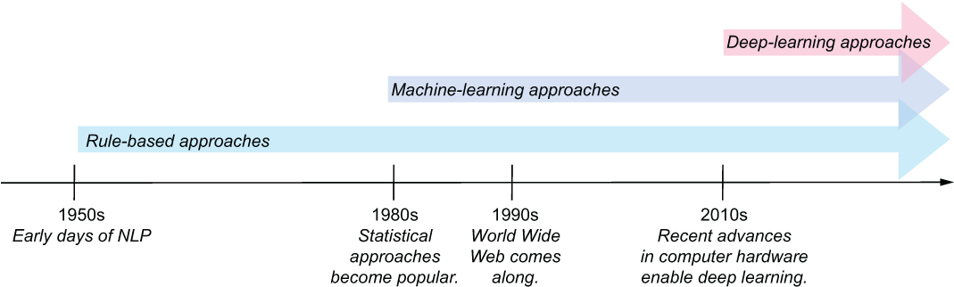
Figure 1.1 NLP timeline showing three different types of approaches

Over the years, NLP got linked to several different fields, and consequently you might come across different aliases, including statistical natural language processing; language and speech processing; computational linguistics; and so on. The distinctions between these are very subtle. What matters more than namesakes is the fact that NLP adopts techniques from a number of related fields:

• Computer science—Contributes with the algorithms, as well as software and hardware

• Artificial intelligence—Sets up the environment for the intelligent machines

• Machine learning—Helps with the intelligent ways of learning from real data

• Statistics—Helps coming up with the theoretical models and probabilistic interpretation

• Logic—Helps ensure the world described with the NLP models makes sense

• Electrical engineering—Traditionally deals with the processing of human speech

• Computational linguistics—Provides expert knowledge about how human language works

• Several other disciplines, such as (computational) psycholinguistics, cognitive science, and neuroscience—Account for human factors, as well as brain processes in language understanding and production

With so many “contributors” and such impressive advances of recent years, this is definitely an exciting time to start working in the NLP area!

1.2 Typical tasks

Before you start reading the next section, here is a task for you: name three to five applications that you use on a daily basis and that rely on NLP techniques. Again, you might be surprised to find that you are already actively using NLP through everyday applications. Let’s look at some examples.

1.2.1 Information search

Let’s start with a very typical scenario: you are searching for all work documents related to a particular event or product—for example, everything that mentions management meetings. Or perhaps you decided to get some from the web to solve the task just mentioned (figure 1.2).

Figure 1.2 You may search for the answer to the task formulated earlier in this chapter on the web.

Alternatively, you may be looking for an answer to a particular question like “What temperature does water boil?” and, in fact, Google will be able to give you a precise answer, as shown in figure 1.3.

Figure 1.3 If you look for factual information, search engines (Google in this case) may be able to provide you with precise answers.

These are all examples of what is in essence the very same task—information search, or technically speaking, information retrieval. You will see shortly how all the varieties of the task are related. It boils down to the following steps:

1. You submit your “query,” the question that you need an answer to or more information on.

2. The computer or search engine (Google being an example here) returns either the answer (like 100°C) or a set of results that are related to your query and provide you with the information requested.

3. If you search for the applications of NLP online, the search engine will provide you with an ordered list of websites that discuss such applications, and if you search for documents on a specific subject on your computer, it will list them in the order of relevance.

This last bit about relevance is essential here—the list of the websites from the search engine usually starts with the most relevant websites that you should visit, even if it may contain dozens of results pages. In practice, though, how often do you click through pages after the first one in the search results? The documents found on your filesystem typically would be ordered by their relevance, too, so you’ll be able to find what you’re looking for in a matter of seconds. How does the machine know in what order to present the results?

If you think about it, information search is an amazing application: First of all, if you were to find the relevant information on your computer, in a shared filesystem at work, or on the internet, and had to manually look through all available documents, it would be like looking for a needle in a haystack. Secondly, even if you knew which documents and web pages are generally relevant, finding the most relevant one(s) among them would still be a hugely overwhelming task. These days, luckily, we don’t have to bother with tasks like that. It is hard to even imagine how much time is saved by the machines performing it for us.

However, have you ever wondered how the machines do that? Imagine that you had to do this task yourself—search in a collection of documents—without the help of the machine. You have a thousand printed notes and minutes related to the meetings at work, and you only need those that discuss the management meetings. How will you find all such documents? How will you identify the most relevant of these?

The first question might seem easy—you need all the documents that contain words like meeting and management, and you are not interested in any other documents, so this is simple filtering, as figure 1.4 shows:

Figure 1.4 Simple filtering of documents into “keep” and “discard” piles based on occurrence of words

Now, it is true that the machines are getting increasingly better at understanding and generating human language. However, it’s not true that they truly “understand” language, at least not in the same way we humans do. In particular, whereas if you were to look through the documents and search for occurrences of meeting and management, you would simply read through the documents and spot these words, because you have a particular representation of the word in mind and you know how it is spelled and how it sounds. The machines don’t actually have such representations. How do they understand what the words are, and how can they spot a word, then?

One thing that machines are good at is dealing with numbers, so the obvious candidate for word and language representation in the “mechanical mind” is numerical representation. This means that humans need to “translate” the words from the representations that are common for us into the numerical language of the machines in order for the machines to “understand” words. The particular representation that you will often come across in natural language processing is a vector. Vector representations are ubiquitous—characters, words, and whole documents can be represented using them, and you’ll see plenty of such examples in this book.

Here, we are going to represent our query and documents as vectors. A term vector should be familiar to you from high school math, and if you have been programming before, you can also relate vector representation to the notion of an array—the two are very similar, and in fact, the computer is going to use an array to store the vector representation of the document. Let’s build our first numerical representation of a query and a document.

Query = "management meeting" contains only two words, and in a vector each of them will get its own dimension. Similarly, in an array, each one will get its own cell (figure 1.5).

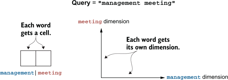
Figure 1.5 In an array, each word is represented by a separate cell. In a vector, each word gets its own dimension.

The cell of the array that is assigned to management will be responsible for keeping all the information related to management, and the cell that is assigned to meeting will similarly be related to meeting. The vector representation will do exactly the same but with the dimensions—there is one that is assigned to management and one that is for meeting. What information should these dimensions keep?

Well, the query contains only two terms, and they both contribute to the information need equally. This is expressed in the number of occurrences of each word in the query. Therefore, we should fill in the cells of the array with these counts. As for the vector, each count in the corresponding dimension will be interpreted as a coordinate, so our query will be represented as shown in figure 1.6.

Figure 1.6 The array is updated with the word counts; the vector is built using these counts as coordinates.

Now, the vector is simply a graphical representation of the array. On the computer’s end, the coordinates that define the vector are stored as an array.

We use a similar idea to “translate” the word occurrences in documents into the arrays and vector representations: simply count the occurrences. So, for some document Doc1 containing five occurrences of the word meeting and three of the word management, and for document Doc2 with one occurrence of meeting and four of management, the arrays and vectors will be as shown in figure 1.7.

Figure 1.7 Arrays and vectors representing Doc1 and Doc2

Perhaps now you see how to build such vectors using very simple Python code. To this end, let’s create a Jupyter Notebook and start adding the code from listing 1.1 to it. The code starts with a very simple representation of a document based on the word occurrences in document Doc1 from figure 1.7 and builds a vector for it. It first creates an array vector with two cells, because in this example we know how many keywords there are. Next, the text is read in, treating each bit of the string between the whitespaces as a word. As soon as the word management is detected in text, its count is incremented in cell 0 (this is because Python starts all indexing from 0). As soon as meeting is detected in text, its count is incremented in cell 1. Finally, the code prints the vector out. Note that you can apply the same code to any other example—for example, you can build a vector for Doc2 as an input using the correspondent counts for words.

Note In this book, by default, we will be using Jupyter Notebooks, as they provide practitioners with a flexible environment in which the code can be easily added, run, and updated, and the outputs can be easily observed. Alternatively, you can use any Python integrated development environment (IDE), such as PyCharm, for the code examples from this book. See https://jupyter.org for the installation instructions. In addition, see the appendix for installation instructions and the book’s repository (https://github.com/ekochmar/Getting-Started-with-NLP) for both installation instructions and all code examples.

Listing 1.1 Simple code to build a vector from text

doc1 = "meeting ... management ... meeting ... management ... meeting "
doc1 += "... management ... meeting ... meeting"    ❶
 
vector = [0, 0]                                     ❷
 
for word in doc1.split(" "):                        ❸
    if word=="management":
        vector[0] = vector[0] + 1                   ❹
    if word=="meeting":
        vector[1] = vector[1] + 1                   ❺
        
print (vector)                                      ❻

❶ Represents a document based on keywords only

❷ Initializes array vector

❸ The text is read in, and words are detected.

❹ Count for “management” is incremented in cell 0.

❺ Count for “meeting” is incremented in cell 1.

❻ This line should print [3, 5] for you.

The code here uses a very simple representation of a document focusing on the keywords only: you can assume that there are more words instead of dots, and you’ll see more realistic examples later in this book. In addition, this code assumes that each bit of the string between the whitespaces is a word. In practice, properly detecting words in texts is not as simple as this. We’ll talk about that later in the book, and we’ll be using a special tool, a tokenizer, for this task. Yet splitting by whitespaces is a brute-force strategy good enough for our purposes in this example.

Now, of course, in a real application we want a number of things to be more scalable than this:

• We want the code to accommodate for all sorts of queries and not limit it to a predefined set of words (like management or meeting) or a predefined size (like array of size 2).

• We want it to properly detect words in text.

• We want it to automatically identify the dimensions along which the counts should be incremented rather than hardcoding it as we did in the code from listing 1.1.

And we’ll do all that (and more!) in chapter 3. But for now, if you grasped the idea of representing documents as vectors, well done—you are on the right track! This is quite a fundamental idea that we will build upon in the course of this book, bit by bit.

I hope now you see the key difference between what we mean by “understanding” the language as humans do and “understanding” the language in a machinelike way. Obviously, counting words doesn’t bring about proper understanding of words or the knowledge of what they mean. But for a number of applications, this type of representation is quite good for what they are. Now comes the second key bit of the application. We have represented the query and each document in a numerical form so that a machine can understand it, but can it tell which one is more relevant to the query? Which should we start with if we want to find the most relevant information about the management meetings?

We used vector representations to visualize the query and documents in the geometrical space. This space is a visual representation of the space in which we encoded our documents. To return the document most relevant to our query, we need to find the one that has most similar content to the query. That is where the geometrical space representation comes in handy—each object in this space is defined by its coordinates, and the most similar objects are located close to each other. Figure 1.8 shows where our query and documents lie in the shared geometrical space.

Figure 1.8 The query (denoted with the circle at [1, 1]) and the documents Doc1 [3, 5] and Doc2 [4, 1], represented in the shared space

The circles on the graph show where documents Doc1 and Doc2 and the query are located. Can we measure the distance between each pair in precise terms? Well, the distance is simply the difference between the coordinates for each of the objects along the correspondent dimensions:

• 1 and 3 along the management dimension for the query and Doc1

• 1 and 5 along the meeting dimension for the query and Doc1

• 1 and 4 along the management dimension for the query and Doc2, and so on

The measurement of distance in geometrical space originates with the good ole Pythagorean theorem that you should be familiar with from your high school mathematics course. Here’s a refresher: in a right triangle, the square of the hypotenuse (the side opposite to the right angle) length equals the sum of the squares of the other two sides’ lengths. That is, to measure the distance between two points in the geometrical space, we can draw a right triangle such that the distance between the two points will equal the length of the hypotenuse and calculate this distance using Pythagorean theorem. Why does this work? Because the length of each side is simply the difference in the coordinates, and we know the coordinates! This is what figure 1.9 demonstrates.

Figure 1.9 In a right triangle, the length of the hypotenuse can be estimated by determining the lengths of the other two sides.

This calculation is called Euclidean distance, and the geometrical interpretation is generally referred to as Euclidean space. Using this formula, we get

ED(query, Doc1) = square_root((3-1)2 + (5-1)2) ≈ 4.47 and 
ED(query, Doc2) = square_root((4-1)2 + (1-1)2) = 3

Now, in our example, we work with two dimensions only, as there are only two words in the query. Can you use the same calculations on more dimensions? Yes, you can. You simply need to take the square root of the sum of the squared lengths in each dimension.

Listing 1.2 shows how you can perform the calculations that we have just discussed with a simple Python code. Both query and document are hardcoded in this example. Then the for-loop adds up squares of the difference in the coordinates in the query and the document along each dimension, using math functionality. Finally, the square root of the result is returned.

Listing 1.2 Simple code to calculate Euclidean distance

import math                                                   ❶
 
query = [1, 1]                                                ❷
doc1 = [3, 5]                                                 ❸
sq_length = 0
 
for index in range(0, len(query)):                            ❹
    sq_length += math.pow((doc1[index] - query[index]), 2)    ❺
            
print (math.sqrt(sq_length))                                  ❻

❶ Imports Python’s math library

❷ The query is hardcoded as [1, 1].

❸ The document is hardcoded as [3, 5].

❹ For-loop is used to estimate the distance.

❺ math.pow is used to calculate the square (degree of 2) of the input.

❻ math.sqrt calculates the square root of the result, which should be ≈ 4.47.

Note Check out Python’s math library at https://docs.python.org/3/library/math.html for more information and a refresher.

Our Euclidean distance estimation tells us that Doc2 is closer in space to the query than Doc1, so it is more similar, right? Well, there’s one more point that we are missing at the moment. Note that if we typed in management and meeting multiple times in our query, the content and information need would not change, but the vector itself would. In particular, the length of the vector will be different, but the angle between the first version of the vector and the second one won’t change, as you can see in figure 1.10.

Figure 1.10 Vector length is affected by multiple occurrences of the same words, but angle is not.

Vectors representing documents can get longer without any conceptually interesting reasons. For example, longer documents will have longer vectors: each word in a longer document has a higher chance of occurrence and will most likely have higher counts. Therefore, it is much more informative to measure the angle between the length-normalized vectors (i.e., vectors made comparable in terms of their lengths) rather than the absolute distance, which can be dependent on the length of the documents.

As you can see in figure 1.10, the angle between the vectors is a much more stable measure than the length; otherwise the versions of the same query with multiple repetitions of the same words will actually have nonzero distance between them, which does not make sense from the information content point of view. The measure that helps estimate the angle between vectors is called cosine similarity, and it has a nice property of being higher when the two vectors are closer to each other with a smaller angle (i.e., more similar) and lower when they are more distant with a larger angle (i.e., less similar). The cosine of a 0° angle equals 1, meaning maximum closeness and similarity between the two vectors. Figure 1.11 shows an example.

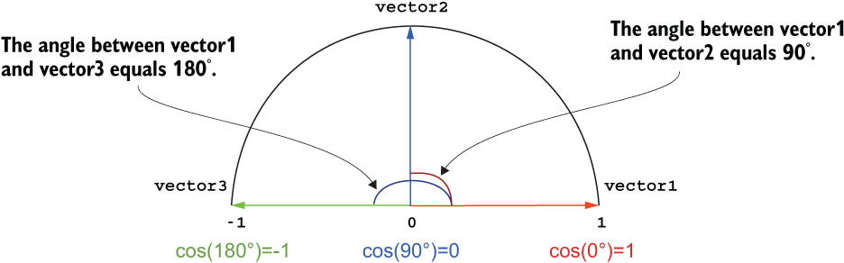
Figure 1.11 The cosine of 0° angle equals 1; vector1 and vector2 are at 90° to each other and have a cosine of 0; vector1 and vector3 at 180° have a cosine of -1.

Vector1 in figure 1.11 has an angle of 0° with itself as well as with any overlapping vectors, so the cosine of this angle equals 1, showing maximum similarity. For instance, the query from our previous examples is maximally similar to itself. Vector1 and vector2 are at 90° to each other, and the cosine of the angle between them equals 0. This is a very low value showing that the two vectors are not similar: as you can see in figure 1.11, it means that the two vectors are perpendicular to each other—they don’t share any content along the two dimensions. Vector1 has word occurrences along the x-axis, but not along y-axis, while vector2 has word occurrences along the y-axis but not along x-axis. The two vectors represent content that is complementary to each other. To put this in context, imagine that vector1 represents one query consisting of a single word, management, and vector2 represents another query consisting of a single word, meeting.

Vector1 and vector3 are at 180° to each other and have a cosine of -1. In tasks based on simple word counting, the cosine will never be negative because the vectors that take the word occurrences as their coordinates will not produce negative coordinates, so vector3 cannot represent a query or a document. When we build vectors based on word occurrence counts, the cosine similarity will range between 0 for the least similar (perpendicular, or orthogonal) vectors and 1 for the most similar, in extreme cases overlapping, vectors.

The estimation of the cosine of an angle relies on another Euclidean space estimation: dot product between vectors. Dot product is simply the sum of the coordinate products of the two vectors taken along each dimension. For example:

dot_product(query, Doc1) = 1*3 + 1*5 = 8
dot_product(query, Doc2) = 1*4 + 1*1 = 5
dot_product(Doc1, Doc2) = 3*4 + 5*1 = 17

The cosine similarity is estimated as a dot product between two vectors divided by the product of their lengths. The length of a vector is calculated in exactly the same way as we did before for the distance, but instead of the difference in coordinates between two points, we take the difference between the vector coordinates and the origin of the coordinate space, which is always (0,0). So, the lengths of our vectors are

length(query) = square_root((1-0)2 + (1-0)2) ≈ 1.41
length(Doc1) = square_root((3-0)2 + (5-0)2) ≈ 5.83
length(Doc2) = square_root((4-0)2 + (1-0)2) ≈ 4.12

And the cosine similarities are

cos(query,Doc1) = dot_prod(q,Doc1)/len(q)*len(Doc1) = 8/(1.41*5.83) ≈ 0.97
cos(query,Doc2) = dot_prod(q,Doc2)/len(q)*len(Doc2) = 5/(1.41*4.12) ≈ 0.86

To summarize, in the general form we calculate cosine similarity between vectors vec1 and vec2 as

cosine(vec1,vec2) = dot_product(vec1,vec2)/(length(vec1)*length(vec2))

This is directly derived from the Euclidean definition of the dot product, which says that

dot_product(vec1,vec2) = length(vec1)*length(vec2)*cosine(vec1,vec2)

Listing 1.3 shows how you can perform all these calculations using Python. The code starts similarly to the code from listing 1.2. Function length applies all length calculations to the passed argument, whereas length itself can be calculated using Euclidean distance. Next, function dot_product calculates dot product between arguments vector1 and vector2. Since you can only measure the distance between vectors of the same dimensionality, the function makes sure this is the case and returns an error otherwise. Finally, specific arguments query and doc1 are passed to the functions, and the cosine similarity is estimated and printed out. In this code, doc1 is the same as used in other examples in this chapter; however, you can apply the code to any other input document.

Listing 1.3 Cosine similarity calculation

import math
 
query = [1, 1]
doc1 = [3, 5]
 
def length(vector):                                            ❶
    sq_length = 0
    for index in range(0, len(vector)):
        sq_length += math.pow(vector[index], 2)                ❷
    return math.sqrt(sq_length)                                ❸
    
def dot_product(vector1, vector2):                             ❹
    if len(vector1)==len(vector2):
        dot_prod = 0
        for index in range(0, len(vector1)):
            dot_prod += vector1[index]*vector2[index]
        return dot_prod
    else:
        return "Unmatching dimensionality"                     ❺
 
cosine=dot_product(query, doc1)/(length(query)*length(doc1))   ❻
print (cosine)                                                 ❼

❶ Function length applies all length calculations to the passed argument.

❷ Length is calculated using Euclidean distance; coordinates (0, 0) are omitted for simplicity.

❸ The code up to here is almost exactly the same as the code in listing 1.2.

❹ Function dot_product calculates dot product between passed arguments.

❺ An error is returned if vectors are not of the same dimensionality.

❻ Specific arguments query and doc1 are passed to the functions.

❼ A numerical value of ≈ 0.97 is printed.

Bits of this code should now be familiar to you. The key difference between the code in listing 1.2 and the code in listing 1.3 is that instead of repeating the length estimation code for both query and document, we pack it up in a function that is introduced in the code using the keyword def. The function length performs all the calculations as in listing 1.2, but it does not care what vector it should be applied to. The particular vector—query or document—is passed in later as an argument to the function. This allows us to make the code much more concise and avoid repeating stuff.

So, in fact, when the length of the documents is disregarded, Doc1 is much more similar to the query than Doc2. Why is that? This is because rather than being closer only in distance, Doc1 is more similar to the query—the content in the query is equally balanced between the two terms, and so is the content in Doc1. In contrast, there is a higher chance that Doc2 is more about “management” in general than about “management meetings,” as it mentions meeting only once.

Obviously, this is a very simplistic example. In reality, we might like to take into account more than just two terms in the query, other terms in the document and their relevance, the comparative importance of each term from the query, and so on. We’ll be looking into these matters in chapter 3, but if you’ve grasped the general idea from this simple example, you are on the right track!

1.2.2 Advanced information search: Asking the machine precise questions

As you’ve seen in the earlier examples, it is not just the documents that you can find by your query—you can also find direct answers to your questions. For example, if you type into your search engine “What temperature is it now?” you may get an answer similar to that shown in figure 1.12.

Figure 1.12 If you type into your search engine a question asking about the temperature, you will get an answer straightaway.

Alternatively, you can test your knowledge on any subject by asking the search engine precise factual questions like “When was the Eiffel Tower built?” or “What temperature does water boil at?” (you saw this last question in figure 1.3). In fact, you’ll get back both the precise answer and the most relevant web page that explains the stuff, as shown in figure 1.13.

Figure 1.13 The search for factual information on Google returns both the precise answer to the question and the accompanying explanation.

Okay, some of the “magic” behind what’s going on should be clear to you now. If the search engine knows that your information need concerns water’s boiling point, it can use information-retrieval techniques similar to the ones we’ve just talked about to search for the most relevant pages. But what about the precise answer? These days you can ask a machine a question and get a precise answer, and this looks much more like machines getting real language understanding and intelligence!

Hold on. Didn’t we say before that machines don’t really “understand” language, at least not in the sense humans do? In fact, what you see here is another application of NLP concerned with information extraction and question answering, and it helps machines get closer to understanding language. The trick is to

• Identify in the natural language question the particular bit(s) the question is about (e.g., the water boiling point).

• Apply the search on the web to find the most relevant pages that answer that question.

• Extract the bit(s) from these pages that answer(s) the question.

Figure 1.14 shows this process.

Figure 1.14 Information extraction pipeline for the query “What temperature does water boil at?”

To solve this task, the machine indeed needs to know a bit more about language than just the number of words, and here is where it gets really interesting. You can see from the example here that to answer the question the machine needs to

• Know which words in the question really matter. For example, words like temperature, water, and boil matter, but what, do, and at don’t. The group {temperature, water, boil} are called content words, and the group {what, do, at} are called function words or stopwords. The filtering is done by stopwords removal, which you’ll learn more about in chapter 3.

• Know about the relations between words and the roles each one plays. For example, it is really the temperature that this question asks about, but the temperature is related to water, and the water is doing the action of boiling. The particular tools that will help you figure all this out are called part-of-speech taggers (they identify that words like water do the action, and the other words like boil denote the action itself) and parsers (they help identify how the words are connected to each other). You will learn more about this in chapter 4.

• Know that boiling means the same thing as boil. The tools that help you figure this out are called stemmers and lemmatizers, and we’ll be using them in this book quite a lot, starting in chapter 3.

As you can see, the machine applies a whole bunch of NLP steps to analyze both the question and the answer, and identify that it is 100°C, and not 0°C or 191°C, that is the correct answer.

1.2.3 Conversational agents and intelligent virtual assistants

When reading about asking questions and getting answers from a machine, you might be thinking that it’s not as frequently done in a browser these days. Perhaps a more usual way to get answers to questions like “Who sings this song?” or “How warm is it today?” now is to ask an intelligent virtual assistant. These are integrated in most smartphones, so depending on the one you’re using, you may be communicating with Siri, Google Assistant, or Cortana. There are also independent devices like Amazon Echo that hosts the Amazon Alexa virtual assistant, which can also be accessed online. There are a whole variety of things that you can ask your virtual assistant, as figure 1.15 demonstrates.

Figure 1.15 A set of questions that you can ask your intelligent virtual assistant (Siri in this case; although you can ask similar questions of Alexa, Google Assistant, or Cortana)

Some of these queries are very similar to those questions that you can type in your browser to get a precise factual answer, so as in the earlier examples, this involves NLP analysis and application of information retrieval and information-extraction techniques. Other queries, like “Show me my tweets” or “Ring my brother at work,” require information retrieval for matching the query to the brother’s work phone number and some actions on the part of the machine (e.g., actual calling). Yet, there are two crucial bits that are involved in applications like intelligent virtual assistants: the input is no longer typed in, so the assistant needs to understand speech, and apart from particular actions like calling, the assistant is usually required to generate speech, which means translating the speech signal internally in a text form, processing the query using NLP, generating the answer in a natural language, and producing output speech signal. This book is on text processing and NLP, so we will be looking into the bits relevant to these steps; however, the speech-processing part is beyond the scope of this book, as it usually lies in the domain of electrical engineering. Figure 1.16 shows the full processing pipeline of a virtual assistant.

Figure 1.16 Processing pipeline of an intelligent virtual assistant

Leaving the speech-processing and generation steps aside, there is one more step related to NLP that we haven’t discussed yet—language generation. This may include formulaic phrases like “Here is what I found,” some of which might accompany actions like “Ringing your brother at work” and might not be very challenging to generate. However, in many situations and, especially if a virtual assistant engages in some natural conversation with the user like “How are you today, Siri?” it needs to generate a natural-sounding response, preferably on the topic of the conversation. This is also what conversational agents, or chatbots, do. So how is this step accomplished?

1.2.4 Text prediction and language generation

If you use a smartphone, you probably have used the predictive keyboard at least once. This is a good realistic example of text prediction in action. If you use a predictive keyboard, it can suggest the next word or a whole phrase for you, based on what you’ve typed in so far. You might also notice that the most appropriate word or phrase is usually placed in the middle for your convenience, and the application learns your individual lingo, so it tries to write as you personally do. In addition, modern technology (e.g., Google’s Smart Reply) allows the machines to respond to emails for you, with usually quite short answers like Either day works for me or Monday works for me. Despite the relative simplicity and shortness of the responses, note how very relevant they usually are! Figure 1.17 provides some examples.

Figure 1.17 On the left: examples of predictive keyboards on smartphones, suggesting the most likely next words or phrases given the context typed in so far. On the right: Google’s Smart Reply for emails.

Before we look under the hood of this application, here’s a short quiz for you. Suppose I provide you with the beginning of a word, for example “langu___,” and ask you “What is the next character?” Alternatively, suppose you can see some words beginning a phrase, for instance “natural language ________.” Can you guess the next word?

I bet your intuition tells you that the first one is almost certainly “language.” The second one might be trickier. You are reading a book on natural language processing, so “processing” might be your most reliable guess. Still, some of you might think of “natural language understanding” or “natural language generation.” These are all valid candidates, but intuitively you know which ones are more likely. How does this prediction work?

Since you use language all the time, you know what events (e.g., sequences of characters or words) occur in language and which ones don’t, and how often they occur relative to each other. This is our human intuitive understanding of probability. In fact, we are so primed to see the expected sequences of characters and words that we easily miss typos and get the main idea from a text even when only the first and the last letter of the word are correct and all other letters are shuffled—for exmaple, you might miss some spleling miskates in this sentence (got it?).

Note Even though the letters in the words example, spelling, and mistakes are shuffled, you probably had no trouble understanding what the sentence is saying. Moreover, if you were reading this text quickly, you might have missed these misspellings altogether. See more examples and explanation for this phenomenon at www.mrc-cbu.cam.ac.uk/people/matt.davis/cmabridge/.

Our expectations are strong and are governed by our observations of what usually happens in language. We make such estimations effortlessly, but machines can also learn about what’s most common in language if they are given such an opportunity. The estimation of what is common and how common it is, is called probability estimation. In practice, you would estimate the probabilities as follows: if we’ve seen 100 contexts where the phrase “natural language ______” was used, and 90 of those were “natural language processing,” 6 were “natural language understanding,” and 4 were “natural language generation,” then you’d say that

Probability("Processing" given "Natural Language" as context) = 90/100 = 90%
Probability("Understanding" given "Natural Language" as context) = 6/100 = 6%
Probability("Generation" given "Natural Language" as context) = 4/100 = 4%

That is, based on what you’ve seen so far (and you make sure that you’ve seen enough and the data that you observed was not abnormal), you can expect 90% of the time to see “natural language processing.” Note that together the estimations add up to 100%. Note also that we can directly compare these probabilities and say that “processing” is more likely given that the beginning of the phrase is “natural language.”

This idea of estimating what is most likely to follow can apply to characters and words. We have been trying to predict the next word or next character based on some previous context. In NLP terms, such context used in prediction is referred to as n-grams, where n represents the number of symbols (i.e., number of characters or words) that are considered as context. For example, l, a, and n in “language” represent character unigrams, while natural, language, and processing in “natural language processing” are word unigrams. Then la, an, and so on are character bigrams, and “natural language” and “language processing” are word bigrams. Trying to predict pairs of characters or words (i.e., bigrams) based on one previous character or word is called bigram modeling, predicting triplets of characters or words based on two previous ones is called trigram modeling, and so on. Figure 1.18 summarizes these examples.

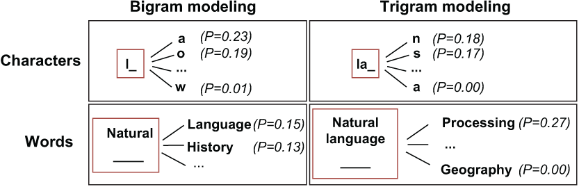
Figure 1.18 Examples of bigram and trigram character and word modeling with probabilities (P)

Why is considering context important, and what is the best n to take into account? Let’s look at our quiz again. If you were given no context to predict, the task of predicting a word or character would be impossible—it could be anything. With one character (e.g., l) or one word (e.g., natural), the number of possibilities is still huge, especially for words. The rules of language do narrow it down for characters: it can be la as in language, le as in lesson, or lo as in local, but few would probably expect it to be lm or lw (unless it’s an abbreviation, of course!). With two previous characters (la) or words (natural language), the correct prediction becomes easier, and for some long contexts (like langu), the possibilities narrow down to one or two options.

This means that the context helps in prediction. That is why we use it and calculate the estimations of probabilities based on it. How far back in context should we look for a reliable prediction, then? It seems like the longer, the better, doesn’t it? Well, there is one more factor to consider: language is really creative. If we take only very long expressions for our probability estimations, we’ll only be able to predict a few of those and will be missing on many more that are probable but have not occurred in exactly the same long context. This is because we will always see fewer examples for the longer expressions than for the shorter ones. If you’ve seen lan ten times, that means that you’ve seen any longer sequence at most ten times. In fact, you might have seen lane two times, land four times, and language four times—so, each of these counts is smaller than ten. But now any sequence longer than four characters starting with lang will be bound to have counts no greater than four, and so on. Ultimately, your probability estimation based on a very long sequence of previous characters, like langua, will return one specific word only. It’s reliable but ultimately not very useful for real language generation.

The problem is particularly obvious with words. Say you’ve seen only one example so far that says “I have been reading this book on natural language processing.” If you were to take the whole sentence as the context (“I have been reading this book on natural __________”) to predict the next word, you will always predict this particular sentence and nothing else. However, if the book is on natural sciences or natural history, or anything else, you won’t be able to predict any of these! At the same time, if you used a shorter context, like “book on natural,” your algorithm would be able to suggest more alternatives. To summarize, the goal is to predict what is probable without constraining it to only those sequences seen before, so the tradeoff between more reliable prediction with longer contexts and more diverse one with shorter contexts suggests that something like two previous words or characters is good enough. Figure 1.19 shows roughly how a text prediction algorithm does its job.

Figure 1.19 Text prediction: a user starts typing a word and the algorithm predicts “language” in the end.

As soon as the user starts typing a word (e.g., starting with a letter l), the machine offers some plausible continuations. Remember, that for convenience, the most probable one is put in the middle: a text prediction algorithm might suggest la (as in last), lo (as in love), or le (as in let’s) as some of the most probable options. The user can then choose the letter that they have in mind. Alternatively, the algorithm can suggest particular words (which most smartphones actually do), like last, love, or let’s. We know that reliable prediction with one character as context is really tricky, and quite probably at this point none of the suggestions are the ones that the user has in mind, so they will continue by typing “la.” At this point, the algorithm uses these two characters as context and adjusts its prediction. It offers lan (or maybe a word like land), las (or last) and lat (or late) as candidates. The user then chooses lan or keeps on typing “lan.” At this point, the machine can both try to predict the word based on characters and check the fit with the previous words. If the user has been typing “I’ve been reading this book on natural lan_____,” both word context and character context would strongly suggest “language” at this point. Figure 1.20 illustrates this process.

Figure 1.20 Language modeling during the learning and prediction phases

This type of prediction based on the sequences of words and characters in context is known as language modeling, and it is at the core of text prediction on your smartphone, or of the Smart Reply technology in your email. It is based on the idea that the sequences of plausible words can be learned in a statistical way—that is, calculating the probabilities on some real data. The data is of paramount importance: both quality and quantity matter. The large quantity of data that became available to the algorithms in the recent decades is one of the strongest catalysts that allowed NLP to move forward and achieve such impressive results. Another is the quality. If you use text prediction on your phone a lot, you might notice that if you had a friend or a colleague named Lang and used this surname quite a lot in messages, your phone will ultimately learn to offer this as the most probable suggestion even if it wasn’t part of the original vocabulary—that is, your phone adapts to your personal vocabulary and uses your own data to do that.

Another factor that contributed to the success of conversational agents and predictive text technology is the development of algorithms themselves. This description would not be complete without mentioning that modern text prediction and chatbots increasingly use neural-based language modeling. The idea is the same—the algorithm still tries to predict the next character or word based on context, but the use of context is more flexible. For instance, it might be the case that the most useful information for the next word prediction is not two characters or words away, but in the beginning of the sentence or in the previous phrase. The n-gram models are quite limited in this respect, whereas more computationally expensive approaches such as neural models can deal with encoding large amounts of information from a wider context and even identify which bits of the context matter more.

Statistical analysis of language, probability estimations, and prediction lie at the core of these and many other applications, including the next ones.

1.2.5 Spam filtering

If you use email (and I assume you do), you are familiar with the spam problem. Spam relates to email that is not relevant to you because, for example, it has been sent to many recipients en masse, or it’s potentially even dangerous, like spreading malicious content or computer viruses or sending links to unsafe websites. Therefore, it is really desirable that such email does not reach your inbox and gets safely put away in the spam or junk folder.

These days, email agents have spam filters incorporated in them, and you might be lucky enough to not see any of the spam emails that are filtered out by these algorithms. Spam filtering is a classic example of an application at the intersection of NLP and machine learning.

To get an idea of how it works, think of something that you would consider to be a spam email. There are several red flags to consider here: an unknown sender, suspicious email address, and unusual message formatting can all be indicative of spam. Ultimately, a lot of what tells you it’s spam is its content. Typically, emails that try to sell you products you have no interest in buying, notify you that you have won a large sum of money in a lottery you have not entered, or tell you that your bank account is blocked (and asks you to click links and submit your personal information) are all very strong clues that the email is spam.

Machine-learning algorithms rely on the statistical analysis and vector representations of text. As before with information search, we represent each email as a vector and call it a feature vector. Each dimension in this vector, as before, represents a particular word or expression, and each such expression is called a feature. The feature occurrences then are counted as before. There is a plethora of machine-learning algorithms, and we will look at some of them in this book, but all they basically do is try to build a statistical model, a function, that helps them distinguish between those vectors that represent spam emails and those that represent normal emails (also known as ham). In doing so, the algorithms figure out which of the features matter more and should be trusted during prediction. Then, given any new email, the algorithm can tell whether it is likely to be spam or ham (figure 1.21).

Figure 1.21 Learning (training) and prediction phases of spam filtering

Spam filtering is one example of a much wider area in NLP—text classification. Text classification aims to detect a class that the text belongs to based on its content. The task may include two classes as with spam filtering (spam versus ham) and sentiment analysis (positive versus negative), or more than two classes: for example, you can try to classify a news article using a number of topics like politics, business, sports, and so on. Several applications we will look into in this book deal with text classification: user profiling (chapters 5 and 6), sentiment analysis (chapters 7 and 8) and topic classification (chapter 9), and your first practical NLP application in chapter 2 will be spam filtering.

1.2.6 Machine translation

Another popular application of NLP is machine translation. Whether you tried to check some information from an international resource (e.g., an unfamiliar term or something reported on the news), tried to communicate with an international colleague, are learning a foreign language, or are a non-native English speaker, you might have relied on machine translation in practice, such as using Google Translate.

As you’ve learned earlier in this chapter, this classic application of NLP has originally been approached in a rule-based manner. Imagine we wanted to translate the text in table 1.1 from English to French and knew how to translate individual words.

Table 1.1 Word-for-word translation between English and French

Can we just put the words together as “applications de naturel langue traitement” to translate a whole phrase? Well, there are several issues with such an approach.

Figure 1.22 Several translations for the English word language to French (Google Translate)

First, when we check the French translations for “language” (as indeed for “applications”), we see several options (figure 1.22). Which one should we choose—is it langue or langage? Second, the translation for natural is not straightforward either. The words seem to have two forms, according to figure 1.23. Again, which one is it? Finally, when we check the translation for the whole phrase, we actually get the one with a different word order (figure 1.24)!

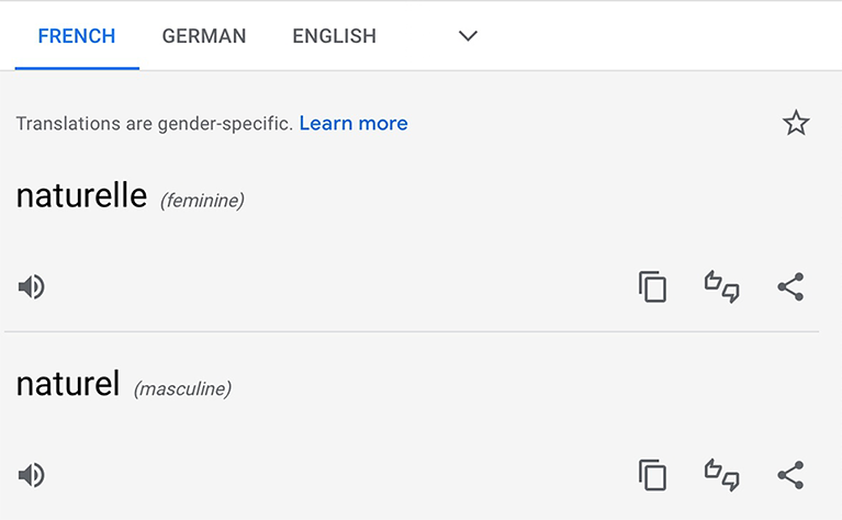
Figure 1.23 The translation of the English word natural to French has two forms, “naturel” and “naturelle” (Google Translate).

Figure 1.24 Phrase translation between English and French for “applications of natural language processing”

We see that several of our assumptions from before were incorrect. First, among the two translations for language, it is langage that should be chosen in this context. Second, French unlike English distinguishes between different genders of words, so if we wanted to choose a form of natural with la langue (“the language”), we’ll have to say naturelle, but with le langage (“the language”), as here, naturel is used. Third, whereas in English adjectives (the words denoting qualities of nouns) like natural come before nouns (the words denoting objects or concepts) like language, in French they follow, thus langage naturel and not naturel langage. Finally, French doesn’t permit saying “natural language processing” and instead requires us to say “processing of natural language,” thus traitement du langage naturel. And, if you are wondering what du means, it is a merger of the words of (de) and the (le).

Now, imagine having to write rules for translating each of these cases from English to French, and then trying to expand the system to other language pairs as well. It would simply not scale! That is why the early rule-based approaches to machine learning took a long time to develop and did not succeed much.

The field, as with other applications, benefited from two things: the spread of statistical approaches to the NLP tasks and the availability of large amounts of data. Around the 1990s, statistical machine translation (SMT) replaced the traditional rule-based approaches. Instead of trying to come up with ad hoc rules for each case, SMT algorithms try to learn from large amounts of parallel data in two languages—that is, the data where the phrases in one language (e.g., natural language on the English side) are mapped to the translated phrases in another language (e.g., langage naturel on the French side). Such mapped parallel data is treated as the training data for the algorithm to learn from, and after seeing lots of phrases of this type in English-French pairs of texts, the algorithm learns to put the adjective after the noun in French translations with high probability.

Obviously, the availability of such parallel data is of paramount importance for the algorithm to learn from, but since there is so much textual information available on the web these days, and many websites have multiple language versions, some of it might be easier to get hold of than before. Finally, this description once again would not be complete without mentioning that neural networks advanced the field of machine translation even further, and the most successful algorithms today use neural machine translation (NMT).

1.2.7 Spell- and grammar checking

One final familiar application of NLP that is worth mentioning is spell- and grammar checking. Whether you are using a particular application, like Microsoft Word, or typing words in your browser, quite often the technology corrects your spelling and grammar for you (try typing “spleling miskates”!). Sometimes it even advises you on how to better structure your sentences by suggesting word order changes and finds better word replacements.

There is a reason we look into this application last: there is a whole bunch of different approaches one can address it with, using a range of techniques that we discussed in this section, so it is indeed a good one to conclude with. Here are some of such approaches:

• Rule-based with the use of a dictionary—If any of the words are unknown to the algorithm because they are not contained in a large dictionary of proper English words, then the word is likely to be a misspelling. The algorithm may try to change the word minimally and keep checking the alternatives against the same dictionary, counting each change as contributing to the overall score or “edit distance.” For example, thougt would take one letter insertion to be converted into thought or one letter substitution to become though, but it will take one insertion and one substitution to become through, so in practice the algorithm will choose a cheaper option of correcting this misspelling to either though or thought (figure 1.25).

• Use of machine learning—Of course, whether it should be though, thought, or through will depend on the context. For example, “I just thougt that even thougt it was a hard course, I’d still look thougt the material” will require all three corrections in different slots. And indeed, one can use a machine-learning classifier to predict the subtle differences in each of the three cases.

• Even better, one can treat it as a machine-translation problem, where the machine has to learn to translate between “bad” English sentences like “I just thougt that even thougt it was a hard course, I’d still look thougt the material” and good ones like “I just thought that even though it was a hard course, I’d still look through the material.” The machine then has to establish the correct translation in each context.

• Use of language modeling—After all, “I just thougt,” “I just though,” and “I just through” are all ungrammatical English and are much less probable than “I just thought.” All you need is a large set of grammatically correct English to let the language-modeling algorithm learn from it.

Figure 1.25 Possible corrections for the misspelling thougt with the assigned edit distances

Now I hope you are convinced that (1) natural language processing is all around you in many applications that you already use on a daily basis; (2) it can really improve your work, in whatever application area you are working in—it’s all about smart information processing; (3) you are already an active user of the technology and, by virtue of speaking language, an expert; and (4) the barrier to entry is low; what might look like a black box becomes much clearer when you look under the hood.

Summary

• Natural language processing is a key component of many tasks.

• NLP has seen a huge boost of interest in the recent years thanks to the development of algorithms, computer software and hardware, and the availability of large amounts of data.

• Anyone working with data would benefit from knowing about NLP, as a lot of information comes in a textual form.

• Knowing about NLP practices will help your application in whatever area you work in. This book will address examples from multiple domains—news, business, social media—but the best way to learn is to identify the project you care about and see how this book helps you solve your task.

• Without consciously thinking about it, you are already an expert in language domain, as anyone speaking language is. You will be able to evaluate the results of the NLP applications, and you don’t need any further knowledge to do that. Furthermore, you have been actively using NLP applications on a daily basis for a long time now!

• One of the key approaches widely used in NLP is “translating” words into numerical representations—vectors—for the machine to “understand” them. In this chapter, you have learned how to do that in a very straightforward way.

• Once “translated” into a numerical form, words, sentences, and even whole documents can be evaluated in terms of their similarity. We can use a simple cosine similarity measure for that.

Solution to exercise 1.1

First, calculate the length of each vector using Euclidean distance between the vector coordinates and the origin (0,0):

length(A) = square_root((4-0)2 + (3-0)2) = 5
length(B) = square_root((5-0)2 + (5-0)2) ≈ 7.07
length(C) = square_root((1-0)2 + (10-0)2) ≈ 10.05

Next, calculate the dot products between each pair:

dot_product(A, B) = 4*5 + 3*5 = 35
dot_product(B, C) = 5*1 + 5*10 = 55
dot_product(C, A) = 1*4 + 10*3 = 34

Finally, for each pair of vectors, take the dot product and divide by the product of their lengths. You have all the components in place for that (figure 1.26):

cos(A,B) = dot_prod(A,B)/len(A)*len(B) = 35/(5*7.07) ≈ 0.99
cos(B,C) = dot_prod(B,C)/len(B)*len(C) = 55/(7.07*10.05) ≈ 0.77
cos(C,A) = dot_prod(C,A)/len(C)*len(A) = 34/(10.05*5) ≈ 0.68

Figure 1.26 The graph shows that vectors A and B are very close to each other, and C is more distant from either of them.