9 Topic analysis

This chapter covers

• Implementing a supervised approach to topic classification with scikit-learn
• Using multiclass classification for NLP tasks
• Discovering topics in an unsupervised way
• Implementing an unsupervised approach—clustering with scikit-learn

In this chapter, you will learn how to automatically detect topics in text, either selecting from the set of known topics or discovering new, previously unseen ones. This is a challenging and practically useful task that can be approached from different perspectives using a variety of methods. This chapter will introduce new techniques, some of which are closely related to the ones that you’ve been using before. Let’s put this task in a broader context before diving deep into the implementation issues.

Previous chapters presented a number of NLP applications that required you to build a machine-learning model that can classify text. Let’s summarize them here:

• In chapter 2, you looked into how to build your own spam filter that can classify incoming email into spam or ham.

• In chapters 5 and 6, you developed an author-identification tool that can detect whether a text is written by one of the known authors (e.g., Jane Austen or William Shakespeare, or one of your contacts should you wish to apply this tool to your own data).

• In chapters 7 and 8, you learned how to build a sentiment analyzer that can classify a text (e.g., a review) as the one expressing a positive or a negative opinion.

All these applications, despite their obvious differences (e.g., detecting that an email is spam or ham is not the same as identifying who it was written by or whether it contains a positive or a negative message), bear a great deal of similarities. These similarities are related to the framework that you use to solve the task. In all these cases, you

• Rely on some data labeled with the classes of interest and build a machine-learning classifier using the classes from the annotated data. Recall that this is called supervised machine learning.

• Aim to distinguish between precisely two types of input (two discrete non-overlapping classes). Recall that this is called binary classification.

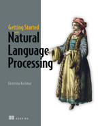
We said before that as soon as you can define separate classes in your data and have data labeled with such classes, you can apply supervised binary classification algorithms. The differences in each particular case will concern the type of features that you would select and the algorithm that you would apply. Figure 9.1 presents the now-familiar machine-learning pipeline for binary classification tasks and highlights the steps that are task-specific.

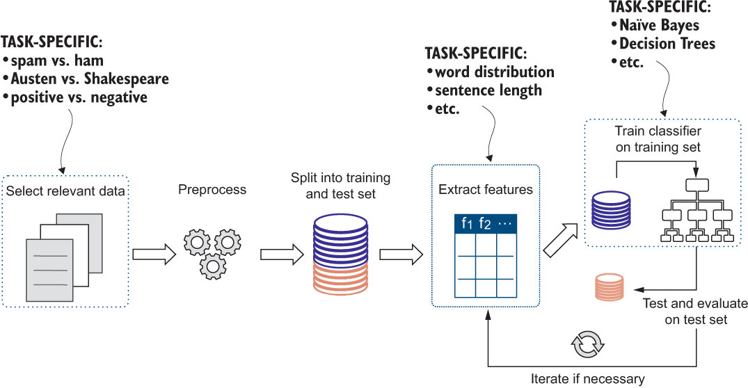
Figure 9.1 Overview of the supervised machine-learning pipeline. The selection of relevant data, feature types, and the algorithm depends on the task, as this diagram highlights.

This powerful approach is applied across the board to a wide range of text classification tasks, of which sentiment analysis, spam detection, and authorship identification are examples familiar to you by now. In this chapter, you will work with one more application of this powerful framework—topic classification. Let’s start with a scenario. Suppose you work as a content manager for a large news platform. Your platform hosts texts from a wide variety of authors and mainly specializes in the following set of well-established topics: Politics, Finance, Science, Sports, and Arts. Your task is to decide, for every incoming article, which topic it belongs to and post it under the relevant tab on the platform. Here are some questions for you to consider:

1. Can you use your knowledge of NLP and machine-learning algorithms to help you automate this process?

2. What if you suspect that a new set of yet-uncovered topics, besides the five just mentioned, started emerging among the texts that authors send you (e.g., you get some articles on the technological advances)? How can you discover such new topics and include them in your analysis?

3. What if you think that some articles lend themselves to multiple topics, which are covered by these articles to a various extent? For instance, some articles may talk about a sports event that is of a certain political importance (e.g., Olympic Games) or about a new technological invention that results in the tech company having high valuation.

This scenario relates to the task that we can broadly define as topic analysis. Question 1 provides you with a hint—it suggests that you already have all the necessary skills and knowledge to use NLP and machine-learning algorithms to classify texts into topics. Indeed, this task is nothing but an extension of the old familiar scenarios where you classified texts into spam versus ham, or positive versus negative, only this time you will need to extend this framework to more than two classes. If you worked as a content manager for this platform before, one can assume that you assigned some articles to each of the categories (topics) in the past. This means that you can easily collect labeled data—just scrape some articles from each of the categories on your platform. Once your labeled data is ready, you can apply a supervised machine-learning algorithm to classify any new article into one of the familiar topics. Since by now you have vast experience working on binary classification applications to various tasks, this is just a small extension step for multiple classes. We will look into this step first, and we’ll call this variety of the task topic classification.

Questions 2 and 3 related to this scenario are more challenging. Imagine that the content on your platform doesn’t stay the same all the time. New topics may emerge in the data. Unfortunately, if you wanted to train a classification model to cover these topics in a supervised manner, you will need labeled articles for these new topics as well. Data availability is the major bottleneck for supervised machine learning. Therefore, in this and the next chapters, you will learn about alternative ways of topic discovery and will apply two unsupervised machine-learning algorithms: clustering, which will be covered in this chapter, and topic modeling with latent Dirichlet allocation (LDA), which will be the topic of the next chapter. The diagram in figure 9.2 summarizes the set of approaches that you will apply to the task of topic analysis.

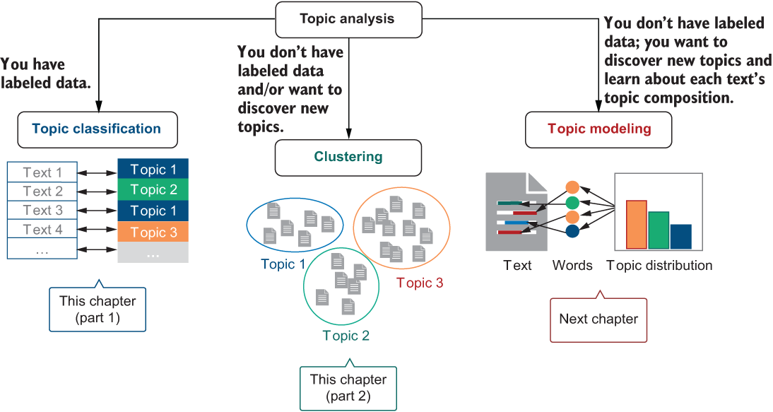
Figure 9.2 Topic analysis using three different approaches. Depending on whether you have labeled data or not, you can apply a supervised or an unsupervised approach (e.g., using clustering, as we’ll cover in this chapter). If you want to discover new topics and learn about text’s topic composition, apply topic modeling (next chapter).

Topic analysis and, in particular, the set of unsupervised approaches to topic discovery, provide you with powerful functionality: you can apply these algorithms to any scenario in which you would like to organize a large collection of documents without spending too much time reading them in detail, be that scientific articles, legal documents, financial documents, patent applications, or emails.

9.1 Topic classification as a supervised machine-learning task

First, let’s approach topic classification using supervised machine learning (ML). By now, you have a lot of experience with supervised ML tasks, only this time you will deal with a problem that has more than two classes. This may sound challenging, but in the course of this section you will see that this is but a small extension step. As is usual with supervised ML tasks, there are several key components to think about: data labeled with the classes of interest, algorithm to apply to this multiclass classification task, and evaluation strategy that will help you check that your approach works well. The mental model in figure 9.3 summarizes these steps. You might recall using this mental model in the previous chapters; this is simply what the supervised machine-learning pipeline looks like. Now let’s look into each of these steps in turn.

Figure 9.3 Mental model for the supervised machine-learning pipeline

9.1.1 Data

Chapter 5 introduced a powerful machine-learning toolkit called scikit-learn that allows you to quickly implement machine-learning applications and use a wide range of out-of-the-box techniques. In this section, you will learn about another useful functionality of this toolkit—the availability of several datasets for your use.

We’ve discussed before that for supervised ML scenarios, high-quality data that is labeled with the classes of interest is of utmost importance. If you are building your own application (e.g., you want to classify your own incoming emails into spam and ham, or you want to analyze your company’s customers reviews), you will have to perform your own data collection and annotation. However, if your main goal is to gain more practice with the use of machine learning and NLP techniques, availability of datasets that are already collected and labeled for you is an important asset. In this chapter, we will use the famous 20 Newsgroups dataset, which is well suited for the topic classification task and is easily accessible via scikit-learn (check scikit-learn’s datasets web page for more information on the various available data: http://mng.bz/yveo).

The 20 Newsgroups dataset is a collection of around 18,000 newsgroups posts on 20 topics (read about this dataset at http://qwone.com/~jason/20Newsgroups/). This dataset has been widely used in the NLP community for various tasks around text classification and, in particular, for topic classification. For the ease of comparison, the dataset is already split into training and test subsets. Table 9.1 summarizes the number of posts in each topic and each subset.

Table 9.1 Full description of the 20 Newsgroups dataset

As you can see, not all newsgroups have a comparable amount of training and test data. Some, like talk.religion.misc and talk.politics.misc, are relatively small. Besides, as you will see later when it comes to visualization of results and evaluation, it might be hard to grasp the results for as many as 20 categories. To this end, let’s select a subset of topics and apply classification to this subset. Luckily, scikit-learn allows you to easily change the set of categories or even include the whole lot of them, so feel free to experiment with your own selection.

Listing 9.1 shows how to initialize the training and test datasets. You start by importing libraries and functions that you will use in this module: specifically, fetch_20newsgroups will help you access the dataset via scikit-learn (See more information on this functionality here: http://mng.bz/M5qD). Next, you define a function load_dataset that will initialize a subset of the data as the train or test chunk of the 20 Newsgroups dataset and will also allow you to select particular categories listed in cats. You need to shuffle the dataset and remove all extraneous information such as footers, headers, and quotes. The code allows you to specify a list of categories of interest. The list of 10 topics here is used as an example. Feel free to select your own. Finally, you initialize newsgroups_train and newsgroups_test subsets. If you use all instead of train or test, you will get access to the full 20 Newsgroups dataset, and None instead of categories will help you access all topics.

Listing 9.1 Code to initialize the newsgroups training and test subsets

from sklearn.datasets import fetch_20newsgroups           ❶
import numpy as np    
 
def load_dataset(a_set, cats):                            ❷
    dataset = fetch_20newsgroups(subset=a_set, categories=cats,
                                remove=('headers', 'footers', 'quotes'),
                                shuffle=True)
    return dataset
 
categories = ["comp.windows.x", "misc.forsale", "rec.autos", "rec.motorcycles", "rec.sport.baseball"]
categories += ["rec.sport.hockey", "sci.crypt", "sci.med", "sci.space", "talk.politics.mideast"]                             ❸
 
newsgroups_train = load_dataset('train', categories)
newsgroups_test = load_dataset('test', categories)        ❹

❶ Import libraries and functions that you will use in this module.

❷ Function load_dataset will access “train” and “test” subsets for particular categories cats.

❸ Define a list of categories of interest.

❹ Initialize newsgroups_train and newsgroups_test subsets.

This code accesses posts from the predefined set of topics only. This can be changed to your own list of topics, or if you want to access all 20 of them, it can be changed to the full list—just use None as the second argument to the function load_dataset. The list of topics that we are going to use in this example is mainly selected based on two factors: diversity of topics and availability of a comparatively large and balanced set of posts across the training and test subsets. Table 9.2 summarizes the data you’ll be working with in this chapter.

Table 9.2 Description of the data from the 20 Newsgroups dataset used in this chapter

In total, you should get a subset of 5,913 training posts and 3,937 test posts. Listing 9.2 shows how to check what data got uploaded and how many posts are included in each subset. In this code, you first check what categories are uploaded using target_names field. This list should coincide with the one that you defined in categories earlier. Then you check the number of posts (filenames field) and the number of labels assigned to them (target field) and confirm that the two numbers are the same. The filenames field stores file locations for the posts on your computer. For example, you can access the first one via filenames[0]. The data field stores file contents for the posts in the dataset; for example, you can access the very first one via data[0]. As a final sanity check, you can also print out category labels for the first 10 posts from the dataset using target[:10].

Listing 9.2 Code to run some general checks on the uploaded data

def check_data(dataset):
    print(list(dataset.target_names))                        ❶
    print(dataset.filenames.shape)
    print(dataset.target.shape)                             ❷
    if dataset.filenames.shape[0]==dataset.target.shape[0]:
        print("Equal sizes for data and targets")           ❸
    print(dataset.filenames[0])                             ❹
    print(dataset.data[0])                                  ❺
    print(dataset.target[:10])                              ❻
 
check_data(newsgroups_train)
print("
***
")
check_data(newsgroups_test)                                  ❼

❶ Check what categories are uploaded using the target_names field.

❷ Check the number of posts (filenames) and the number of labels assigned to them (target).

❸ Confirm that the two numbers above are the same.

❹ The filenames field stores file locations for the posts on your computer.

❺ The data field stores file contents for the posts in the dataset.

❻ Print out category labels for the first 10 posts from the dataset using target[:10].

❼ Apply this function to newsgroups_train and newsgroups_test.

The code in the listing produces the following output:

['comp.windows.x', 'misc.forsale', 'rec.autos', 'rec.motorcycles', 'rec.sport.baseball', 'rec.sport.hockey', 'sci.crypt', 'sci.med', 'sci.space', 'talk.politics.mideast']
(5913,)
(5913,)
Equal sizes for data and targets
/[Your_home_directory]/scikit_learn_data/20news_home/20news-bydate-train/rec.sport.baseball/102665
I have posted the logos of the NL East teams to alt.binaries.pictures.misc 
 [...]
 
[4 3 9 7 4 3 0 5 7 8]
 
***
 
['comp.windows.x', 'misc.forsale', 'rec.autos', 'rec.motorcycles', 'rec.sport.baseball', 'rec.sport.hockey', 'sci.crypt', 'sci.med', 'sci.space', 'talk.politics.mideast']
(3937,)
(3937,)
Equal sizes for data and targets
/[Your home directory]/scikit_learn_data/20news_home/20news-bydate-test/misc.forsale/76785
As the title says. I would like to sell my Star LV2010 9 pin printer.
[...]
 
[1 7 2 5 3 5 7 3 0 2]

The first half of this printed output is related to the training data, and the second one to the test data. To help you understand this output better, figure 9.4 first visualizes how the data is stored and how it can be accessed, and the description following it provides you with more detail.

Figure 9.4 Data representation in the scikit-learn’s 20 Newsgroups dataset. The dataset is stored as a dataset object, with various methods available to access different types of information; for example, target_names returns the topic labels, while target presents them in a numerical format; filenames tells you where on your computer the files are stored, while data shows the content of the posts. This way, you can extract any information you need from the dataset object.

In the first line of the output, you see that the categories have been loaded correctly. The number of posts in the training data is equal to 5913, and in the test data to 3937, as expected. Since dataset.filenames returns a list and dataset.target returns an array, when you check their shape you see, for example, (5913, ). This notation means that the particular data structure has a single dimension to the length of 5913 (e.g., it is a list or an array of 5,913 elements). As a side note, if shape output is of the form (m, n), it means that you are working with a two-dimensional data structure—a matrix of m rows and n columns.

Note that scikit-learn allows you to not only access the dataset, but it also represents it as an object with relevant attributes that can be directly accessed via dataset.attribute. For example:

• target_names returns the list of the names for the target classes (categories).

• filenames is the list of paths where the files are stored on your computer.

• target returns an array with the target labels (note that the category names are cast to the numerical format).

• data returns the list of the contents of the posts (see http://mng.bz/M5qD).

The list of targets represents categories numerically. This is because machine-learning classifiers implemented in scikit-learn prefer to work with numerical format for the labels. Numbers are assigned to categories in alphabetical order: for instance, 'comp.windows.x' corresponds to the numerical label 0, 'misc.forsale' to 1, and so on. An output like [4 3 9 7 4 3 0 5 7 8] tells you that the posts on different topics are shuffled: the first one is on rec.sport.baseball, the second one is on rec.motorcycles, and so on (you can check the order of the categories in table 9.2).

9.1.2 Topic classification with Naïve Bayes

Now that the data is uploaded, let’s turn to machine-learning techniques with scikit-learn, train a classifier on the training data, and try to predict the topic labels on the test data. As before, the next step in an ML project is to select features to be used with your classifier.

These considerations should help you decide upon the type of features—you should start by using words. The next point to consider is word selection—are all words equally helpful in topic classification? For instance, you’ve seen before that stopwords are useful in the writing style (or authorship) detection, as people use them differently and in different proportions, but given that all Newsgroups texts are posts of a relatively similar style, it is safe to assume that stopwords are not helpful and can be removed.

Finally, how should features be represented? For instance, should you assume that all words are equally important and therefore should just be simply counted? Topic classification task on the basis of word occurrences boils down to recognizing which topic a text may belong to based on which words are used in this text. Try solving the word puzzles in exercise 9.2 to see how an ML classifier may detect a topic.

So far so good, but note that, compared to the previous applications, we’ve made the detection task more complex. We are considering 10 topics and a vast range of words (all but stopwords) occurring in newsgroups posts. Many of these words will occur not in a single topic but rather across lots of posts on various topics. Consider a word post as one example of a frequent and widely spread word: it might mean a new post that someone has got and, as such, might be more relevant to the texts in the talk.politics .mideast topic. At the same time, you will also see it frequently used in contexts like “I have posted the logos of the NL East teams to . . .” That is, despite the word post not being a stopword, it is quite similar to stopwords in nature. It might be used frequently across many texts on multiple topics, and thus lose its value for the task. How can you make sure that words that occur frequently in the data are given less weight than more meaningful words that occur frequently in a restricted set of texts (e.g., restricted by a topic)?

Figure 9.5 visualizes this idea, representing stopwords (e.g., “this” or “of”) in regular font and highlighting the words that are specific to a particular topic (e.g., “car” for rec.autos or “launch” for sci.space) in italics and those that are distributed widely across all topics (e.g., “post” or “attend”) in bold.

Figure 9.5 Examples of two posts, with stopwords in regular font, words that are distributed widely across multiple topics in bold, and words that are most indicative of a specific topic in italics

In fact, you have already come across a technique that allows you to downweigh terms that occur frequently across many documents and upvalue terms that occur frequently only in some documents but not across the whole collection. This technique is called term frequency —inverse document frequency (TF-IDF), and it was discussed in detail in chapter 3. Here is a reminder:

• You would like to ensure that each word’s contribution is not affected by the document length. For instance, a post with 100 words may use a word car 2 times, while another post of 200 words may use car 4 times. It might seem as if the post with 4 occurrences of car is more focused on cars, but once you take into account the overall length of text, you notice that the actual contribution of car in both cases is tf(“car”) = 4/200 = 2/100 = 0.02. This is what term frequency allows you to deduce.

• You would also like to ensure that word contribution is measured against its specificity. As the previous example shows, if you see a word post in virtually every text, its contribution should be lower than a contribution of some more topical words like car. This is what inverse document frequency allows you to take into account: if a word post is used in 80 posts out of 100, and car is used in 25 posts out of 100, then idf(“post”) = 100/80 = 1.25 < idf(“car”) = 100/25 = 4 (i.e., car has much more weight by way of being less widely spread across the collection of texts).

• Finally, putting the two bits together, TF-IDF = tf*idf gives higher weights to words that are used frequently within some documents but not across a wide variety of documents. This technique, therefore, is very useful for our task at hand.

Application of the TF-IDF technique to raw word counts is quite straightforward in scikit-learn. You’ve already used some vectorizers—functions that are capable of counting word occurrences in texts and then presenting each text as a vector of such word counts. For instance, CountVectorizer that you used in chapter 8 did exactly that (see more information on the CountVectorizer at http://mng.bz/aJG9). Here you are going to learn how to use another type of vectorizer, TfidfVectorizer (the documentation can be found at http://mng.bz/gwW8). As its name suggests, TfidfVectorizer performs word counting and TF-IDF weighing in one go. Listing 9.3 shows how to use it. First, you initialize the vectorizer to apply to all words but stopwords. The vectorizer estimates word counts and learns the tf-idf weights on the training data (thus method .fit_transform is applied to the train_set) and then applies the weights to the words in the test data (this is done using method .transform applied to the test_set). Using the vectorizer, you convert training and test texts into vectors and store the resulting vectors as vectors_train and vectors_test. In the end, you can run some checks on the vectors; for example, check the dimensionality of the vector structures using .shape, see how the first training text is represented, and check which word corresponds to a particular ID (33404 in this code).

Listing 9.3 Code to apply TfidfVectorizer and convert texts into vectors

from sklearn.feature_extraction.text 
import TfidfVectorizer                                      ❶
 
vectorizer = TfidfVectorizer(stop_words = 'english')        ❷
 
def text2vec(vectorizer, train_set, test_set):
    vectors_train = vectorizer.fit_transform(train_set.data)
    vectors_test = vectorizer.transform(test_set.data)      ❸
    return vectors_train, vectors_test
 
vectors_train, vectors_test = text2vec(
    vectorizer, newsgroups_train, newsgroups_test)          ❹
 
print(vectors_train.shape)
print(vectors_test.shape)
print(vectors_train[0])
print(vectorizer.get_feature_names()[33404])                ❺

❶ Import TfidfVectorizer.

❷ Initialize the vectorizer to apply to all words but stopwords.

❸ The vectorizer estimates TF-IDF weights on the training data and then applies them to the test data.

❹ Convert training and test texts into vectors and store the results.

❺ Run some checks on the vectors; use get_feature_names_out in newer versions of scikit-learn.

The preceding code returns the following output ([...] shows that there are more words included in the first text, but we omit them here for space reasons):

(5913, 52746)
(3937, 52746)
  (0, 15218)  0.31618146678372416
  (0, 50534)  0.20153071455804605
  (0, 50435)  0.1817612919269656
  [...]
nl

The first two lines tell you that vectors_train is a matrix of 5,913 rows and 52,746 columns, while vectors_test is a matrix of 3,937 rows and 52,746 columns. You can imagine two large tables here, with each of the rows representing a text (remember, there are 5,913 training posts and 3,937 test posts) and each column representing a word. It is no coincidence that both matrices contain the same number of columns. The TfidfVectorizer identified 52,746 non-stopwords in the training data, and it is this set of words that is used to classify texts into topics here. The method fit_transform then calculates TF-IDF scores based on the training texts (with the fit part of the method) and transforms the raw counts in the training data to these scores. Finally, it applies the same transformations to the occurrences of the same 52,746 words in the test data (with the transform method). It is important that the TF-IDF scores are learned on the training set only. This is why we only use transform method on the test data and do not apply fit_transform, as this will rewrite our TF-IDF scores based on the test data, and we will end up with two separate sets of TF-IDF scores—one fit to the training data and another to the test data. Remember that in a real-life application, you would have access only to the training data and your test set might come, for example, from the future posts on your news platform.

A glimpse into the first text from the training set shows a list of references and scores. For example (0, 15218) with a rounded-up score of 0.32. This representation means that (0, 15218) refers to the first text (thus, the index of 0) and 15218 is the index of the 15,219th word in the total set of 52,746 words used for classification. Which word does it correspond to? You can always check this by applying vectorizer .get_feature_names()[index] (or vectorizer.get_feature_names_out()[index] in newer versions of scikit-learn) as you do in the code above for the 33,405th word (which turns out to be nl used in NL East teams that you can see in the output for listing 9.2). That is, the vectorizer collects 52,746 words, orders them alphabetically, assigns a unique identifier to each word, and finally estimates the TF-IDF score (for the 15,219th word, it is roughly 0.32). Figure 9.6 visualizes how the first training text is represented in the vectors_train structure.

Figure 9.6 A glimpse into the text vector for the first post in the training data. You can see what word each ID corresponds to and how highly it is weighted by TF-IDF.

Now that the data is prepared and converted to the same format with the TF-IDF weights applied to the same vocabulary of words in the training and test posts, let’s train the Naïve Bayes classifier as you did in the previous applications and classify the posts from the test set into topics. Listing 9.4 shows you how to do that.

Listing 9.4 Code to perform topic classification with the Naïve Bayes classifier

from sklearn.naive_bayes import MultinomialNB   ❶
 
clf = MultinomialNB(alpha=0.1)                  ❷
clf.fit(vectors_train, newsgroups_train.target)
predictions = clf.predict(vectors_test)         ❸

❶ Import MultinomialNB.

❷ Initialize the algorithm. The alpha parameter controls smoothing.

❸ Train the algorithm on the training data and return the predictions on the test data.

This training and testing routine should look pretty familiar to you by now. There is only one new parameter, alpha, that this code specifies for the Naïve Bayes algorithm, which we haven’t discussed before. Let’s see what this parameter does.

Imagine the following situation (we will be using a very small number of word occurrences to make the example simple, but you can scale this example up to larger numbers): the set of words that you use for classification contains ["car", "dealer", "engine", "post", "speed", . . .], among others. Imagine that you are working with a small training set, and the whole training set on the automotive topic contains the occurrences for the words as shown in table 9.3.

Table 9.3 An example of word counts in the automotive topic

The probability that a particular word occurs in a text on a particular topic is estimated on the training data using the number of times a word occurs divided by the total number of all word occurrences in this topic. As table 9.3 shows, if you see car in the automotive texts 10 times while the sum of all word occurrences in these texts equals 20, we say that with the probability 10/20 = 0.50 (i.e., with a 50% chance), a text on the automotive topic will include the word car. At the same time, in your small training data, you have never seen a word post used in a text on the automotive topic, so its probability is 0. That may be fair enough—perhaps posts are never discussed in texts that talk mainly about cars.

However, earlier we said that actually a word like post may well occur across various topics. Now imagine your test set contains a text with the following sentence: “This is a post about my car”. Most words here are stopwords, but two words—post and car—are part of the training set vocabulary. Let’s estimate the probability that this text belongs to the automotive topic. For that, we take the probabilities that the words originate with this topic (the ones that you’ve estimated in table 9.3) and multiply them: P(this text is about cars) = P(texts on cars) * P("car" occurs in a text on cars) * P("post" occurs in a text on cars). This formula follows the Naïve Bayes estimation that we discussed in chapter 2. Recall that the first probability is our expectation to see a text on the automotive topic in general. For example, if our training data contains 100 texts, with 10 texts on each of the 10 topics, P(texts on cars) = 10/100 = 0.1, or 10%. Let’s multiply our probabilities now:

P(this text is about cars) = 
P(texts on cars) * P("car" occurs in a text on cars) * P("post" occurs in a text on cars) =
0.1 * 0.5 * 0.0 = 0.0

In other words, despite the fact that this text contains a highly probable word from the automotive topic (car), it now has zero chances of being classified with the automotive topic because it also contains the word post, which has zero probability of occurring in texts on cars simply because you’ve never seen it occurring in automotive texts in the training data! Here is the problem with this data-driven approach to the probability estimation: if you haven’t seen a word (e.g., post) in texts on a specific topic (e.g., texts on cars) in the training data, you might assume it is impossible to ever see this word in texts on this topic; however, it is actually much more likely that you haven’t seen this word simply because you have too small or not diverse enough training data. In practice, it is very hard to make sure that you’ve seen all the possible texts on a specific topic (or all possible events in any supervised ML task). However large and diverse your training set is, there is always a chance that you haven’t (yet) seen some examples. What can you do to fix this? Figure 9.7 proposes a solution, which is then elaborated in more detail.

Figure 9.7 To avoid zero probabilities for some words, which is often caused by not having diverse or large enough training data, we can “pretend” that we have seen each word a bit more frequently than we did, such as by adjusting all word counts by 1.

A technique that is often used in practice is called smoothing and it helps ensure that you don’t end up with zero probability estimates as occurred earlier because of the data effects. The most straightforward approach is called additive or Laplace smoothing (see chapter 3.5 in https://web.stanford.edu/~jurafsky/slp3/3.pdf) and here is how it works: instead of working with the actual counts, some of which might be zeros, let’s pretend that we’ve seen every word a bit more frequently than we actually did. That is, if you’ve never encountered the word post in the texts on cars, you should pretend that you’ve seen it, for instance, once. Such an adjustment is called add-one smoothing, and it is a type of Laplace smoothing. Note in figure 9.7 that the table on the left contains actual word counts from the data and has 0 for post, while the table on the right contains adjusted word count and, thus, 1 for post. However, it would be unfair to only increment the counts for previously unseen words. The new count for post will now be 1, but what about the words that you’ve actually seen once in the data? To make it a fair play for all words, you need to increment the counts for each word in a similar way. All words that you’ve seen once will get a new count of 2, twice 3, and so on. Let’s update the counts from table 9.3 with this add-one technique. Note that the table on the left in figure 9.7 corresponds to table 9.3, and the table on the right in figure 9.7 corresponds to table 9.4.

Table 9.4 Word counts and probabilities updated with add-one smoothing

Two observations are due: first of all, note that all probability values from table 9.3 sum up to 1 (0.50 + 0.10 + 0.25 + 0.00 + 0.15 = 1.00) and so do the probability values in table 9.4 (0.44 + 0.12 + 0.24 + 0.04 + 0.16 = 1.00). This is important because it still allows you to say things like “If a text is on the automotive topic, the most probable word you will see is car,” and it also allows you to reason about the word occurrence with a proper probability distribution. Note that you achieve this by adjusting the total number of all word occurrences from 20 (actual counts) to 25 (counts that take all add-ones into account). The second observation is that, even though the adjusted probabilities are different from the original ones, the total order doesn’t change: P(car) > P(engine) > P(speed) > P(dealer) > P(post) in both cases. It might seem like the changes to some probabilities (e.g., for the most frequent word car, it is -0.06 from 0.50 to 0.44, and the unseen one post, it is +0.04 from 0.00 to 0.04) are more radical than to others (e.g., for the words in the middle range like speed, +0.01 from 0.15 to 0.16). This is because the method redistributes the probabilities between all the words, “borrowing” the probability mass from the more frequent words and “donating” it to the less frequent ones, thus smoothing the probability across the whole range. In this toy example, we see quite radical changes of -0.06 or +0.04 because we are looking into a small word set with very few words and small counts. In real examples, the changes won’t be that radical. The precise amount of probability to redistribute is controlled by the parameter alpha in the code in listing 9.4, and as the code shows, it can take values different from 1.

Finally, if you now want to estimate the probability of the text that says “This is a post about my car” belonging to the automotive topic, you will get the following:

P(this text is about cars) = 
P(texts on cars) * P("car" occurs in a text on cars) * P("post" occurs in a text on cars) =
0.1 * 0.44 * 0.04 = 0.00176

This is what the alpha parameter allows you to do without explicitly adding anything to the counts yourself. Note that unlike in our toy example, in the actual task you are working with as many as 52,746 words (features), and the algorithm relies not on the raw word occurrences but on the TF-IDF scores. Unlike in our toy example, alpha does not have to be an integer number and does not have to be precisely 1. For instance, it is set to 0.1 in the code. You might be wondering what happens if you don’t specify this parameter. In fact, scikit-learn takes care of that and assumes alpha=1.0 by default. Finally, you might be wondering what the best setting for alpha is, then. In practice, you would experiment with various settings for this parameter to select the one that works best for your task, but this type of experimentation is outside the scope of this chapter.

Note Technically, alpha here is called a hyperparameter. It is a setting of the algorithm that is decided upon prior to training the algorithm and building the ML model. That’s why if you would like to find the optimal setting for alpha depending on your task and data, you would do that in a separate set of experiments prior to training Naïve Bayes.

9.1.3 Evaluation of the results

Finally, it is time to evaluate the results obtained when you apply your model to the test set.

You may recall from previous chapters that accuracy is a widely used metric that helps you evaluate the performance of your algorithm at a glance; however, it doesn’t tell you how well your algorithm performs on each class in particular. In contrast, precision, recall, and F-score are metrics applicable to each class and provide you with a more fine-grained insight into the performance. Let’s apply these metrics to your algorithm’s output, and let’s also investigate which words are the most informative when detecting each topic. Listing 9.5 explains how to do that. In this code, you rely on scikit-learn’s metrics functionality, which allows you to quickly evaluate your output. To identify the most informative features in each category, you first iterate through the categories using enumerate(categories). This allows you to iterate through the tuples of (category id, category name). Within this loop, classifier.coef_[i] returns a list of probabilities for the features in the i-th category, and np.argsort sorts this list in the increasing order (from the smallest to the largest) and returns the list of identifiers for the features (see NumPy’s documentation at http://mng.bz/e79G). As a result, you can extract n most informative features using [-n:] (see additional code examples at http://mng.bz/pOnR). You can access the word features via their unique identifiers using vectorizer.get_feature_names() and print out the name of the category and the corresponding most informative words. In the end, you print out the full classification_report and the top 10 informative features per category.

Listing 9.5 Code to evaluate the results for this approach

from sklearn import metrics                                   ❶
 
def show_top(classifier, categories, vectorizer, n):
    feature_names = np.asarray(vectorizer.get_feature_names())
    for i, category in enumerate(categories):                 ❷
        cat_features = classifier.coef_[i]                    ❸
        top = np.argsort(cat_features)[-n:]                   ❹
        print(
            f'{category}: {" ".join(feature_names[top])}'
        )                                                     ❺
        
full_report = metrics.classification_report(newsgroups_test.target, 
                                predictions,
                                target_names=newsgroups_test.target_names)
print(full_report)
show_top(clf, categories, vectorizer, 10)                     ❻

❶ Import scikit-learn’s metrics functionality that will allow you to quickly evaluate your output.

❷ Iterate through the categories using enumerate(categories).

❸ classifier.coef_[i] returns a list of probabilities for the features in the i -th category.

❹ np.argsort sorts this list in the increasing order and returns the list of identifiers for the features.

❺ Access the word features via their unique identifiers and print out the category and the most informative words.

❻ Print out the full classification_report and the top 10 informative features per category.

This code returns the results as shown next. The first part of the output is presented as a table for better readability (table 9.5). Also note that some results are removed from the printout for space reasons since the performance across categories is quite similar.

Table 9.5 Classifier performance across categories

comp.windows.x: program using application windows widget use thanks motif server window
misc.forsale: asking email sell price condition new shipping offer 00 sale
rec.autos: know don new good dealer engine just like cars car
rec.motorcycles: don helmet riding just like motorcycle ride bikes dod bike
rec.sport.baseball: braves pitching hit think runs games game baseball team year
rec.sport.hockey: think year nhl season games players play hockey team game
sci.crypt: escrow people use nsa keys government clipper chip encryption key
sci.med: cadre dsl chastity n3jxp skepticism banks pitt geb gordon msg
sci.space: lunar just shuttle earth like moon orbit launch nasa space
talk.politics.mideast: just said arab turkish armenians people armenian jews israeli israel

The top of this printout should look familiar by now. Each row corresponds to a different category, and each column reports a different metric. Precision values range between the minimum of 0.71 for rec.sport.hockey to 0.92 for comp.windows.x, rec.sport.baseball, and sci.med. Recall values are also pretty high: from 0.78 for rec.autos to 0.94 for rec.sport.hockey. As the F1-score reports a balanced value combining both precision and recall, unless you have a reason to believe one of the two is more important as a metric for your application, it is the F1-score that you should look into. The numbers here are also quite good. The lowest F1-score of 0.80 is observed on rec.autos, and this is due to the somewhat lower recall of 0.78. Lower recall means that not all posts on rec.autos have been detected by your algorithm: 0.22 of the total amount of these posts were erroneously classified as some other topic(s).

The highest F1-score is observed on comp.windows.x, and this is because both precision (0.92) and recall (0.90) are high. This topic seems to be the most easily identifiable one. The Support column provides you with the absolute number of posts in each category. Finally, at the bottom of this bit of the printout you see the accuracy value of 0.85, and the two types of averaged values for all other metrics. Macro average calculates the values summing over the scores for all categories and dividing the sum by 10 (the number of categories), while the weighted average also takes into account the number of instances in each category, thus making sure that the contribution of each category to the average is proportionate to the category size. In this case, both sets of values are identical. This is because our categories are quite balanced in terms of their sizes, ranging from 376 posts in the talk.politics.mideast category to 399 in rec.sport.hockey (the difference is relatively small).

At the bottom of this printout, you see lists of the 10 most informative words from each category. These are the words that have the highest probabilistic weights in each category, so the classifier “trusts” them a lot when the decision about the category of a post is made. Do these word lists align with your expectations about what each topic describes? In other words, going back to exercise 9.2, if you saw a list containing words like [escrow, people, use, nsa, keys, government, clipper, chip, encryption, key], would you guess “cryptography” as the topic?

To finish with the analysis of the results, let’s analyze the classifier’s errors. Start with exercise 9.4.

The code in listing 9.6 shows how to explore the confusions that the classifier makes. In this code, you rely on scikit-learn’s plot_confusion_matrix functionality and matplotlib’s plotting functionality. The plot_confusion_matrix’s functionality allows you to plot the predictions that the classifier makes on vectors_test against the actual labels from newsgroups_test.target using a heatmap. Additionally, you can set some further parameters; for instance, represent the number of correct and incorrect predictions using integer values format (i.e., values_format="0.0f") and highlight the decisions on the heatmap with a particular color scheme. In this code, you use a blue color scheme, with the darker color representing higher numbers. Finally, you print out the confusion matrix and visualize correct predictions and confusions with a heatmap. For reference, you can also print out the categories’ IDs that correspond to the categories’ names.

Listing 9.6 Code to explore the classifier’s errors and confusions

from sklearn.metrics import plot_confusion_matrix
import matplotlib.pyplot as plt                               ❶
 
classifier = clf.fit(vectors_train, newsgroups_train.target)
 
disp = plot_confusion_matrix(classifier, vectors_test, 
                            newsgroups_test.target,           ❷
                            values_format="0.0f",             ❸
                            cmap=plt.cm.Blues)                ❹
    
print(disp.confusion_matrix)                                  ❺
 
plt.show()                                                    ❻
for i, category in enumerate(newsgroups_train.target_names):
    print(i, category)                                        ❼

❶ Import sklearn’s plot_confusion_matrix functionality and matplotlib’s plotting functionality.

❷ Plot the predictions that the classifier makes on vectors_test against the actual labels.

❸ Represent the number of correct and incorrect predictions using integer values format.

❹ Highlight the decisions with a particular color scheme with darker colors for higher numbers.

❺ Print out the confusion matrix.

❻ Visualize correct predictions and confusions.

❼ For reference, print out the categories’ IDs that correspond to the categories’ names.

This code produces the output shown in figure 9.8:

Figure 9.8 The output produced by listing 9.6

As you can see from the confusion matrix, category 2 (rec.autos) indeed has the lowest number of posts (308) that are correctly assigned to this topic. In fact, some of the posts from this category end up being classified into all of the other topics: most notably, 25 posts end up in category 3 (rec.motorcycles), which may not be very surprising given the similarity of the two categories; 27 posts in category 5 (rec.sport.hockey), which is more surprising; and a smaller number of posts being erroneously assigned to other categories. It is also clear from this confusion matrix why precision on category 5 (rec.sport.hockey) is relatively low. Follow the numbers in the sixth column, and you will see that some texts from all other topics end up in this category, including 27 posts from rec.autos, 33 from rec.sport.baseball, 18 from sci.crypt, 17 from sci.med, 18 from sci.space, and so on.

Despite these classification errors, note that the overall performance of this relatively simple algorithm is quite high: 0.85 for both the accuracy and average F1-score on a 10-class prediction task. Congratulations, you have successfully built a supervised machine-learning topic classifier! This is a good starting point for an application for which you have a sufficient number of texts already labeled with their topics. What should you do if that’s not the case?

9.2 Topic discovery as an unsupervised machine-learning task

It’s time now to turn to the second paradigm of machine-learning approaches—unsupervised machine learning. This family of approaches is suitable for situations when you don’t have labeled data and need to learn about the patterns from the data itself. So far, for a number of NLP applications we’ve looked into, we’ve been working under the assumption that labeled training data is easy to come by. In many real-life applications this is not the case, so let’s now consider what happens if you keep receiving new texts for your news platform, but you believe that either the set of topics is not exactly the same as it used to be, or maybe new topics that you don’t have the labeled data for yet keep cropping up. Why not try to learn about these topics from the texts themselves?

Figure 9.9 presents the mental model for the application of unsupervised approaches. In this section, we will look into each step of this process, starting with the selection of an appropriate algorithm.

Figure 9.9 Mental model for the application of unsupervised approaches to NLP tasks. As before, you start with the selection of the input data and extract informative features. High dimensionality of the input data may be a problem for unsupervised ML algorithms, so once the dimensionality is reduced, you can apply a suitable algorithm. Finally, you should evaluate the results with an appropriate set of metrics.

9.2.1 Unsupervised ML approaches

Let’s first discuss how unsupervised approaches work in general and then see how we can apply them to language tasks. Imagine the following scenario: suppose you are given a fruit basket and are asked to build an algorithm that can automatically sort fruits in the basket by type, so that, for example, apples will end up in one pile, oranges in another, and so on. All you know about the basket contents is that it contains fruits; you don’t know which particular types of fruits are in there, and you’d like to build a general enough algorithm that can distinguish between any types of fruit based on their characteristics.

This is a perfect scenario for an unsupervised ML algorithm. Note that if you want to be able to distinguish between any types of fruit, you essentially assume you are not working with any specific labeled data. How can you approach this task?

First, note that you want to be able to distinguish between fruits based on their characteristics. You might come up with the following set of characteristics: [color, size, weight, shape, taste], and perhaps some others. You can see that there comes some similarity between this approach and supervised approaches. In supervised ML, you would have used similar characteristics as features. The difference is that without labeled data, the algorithm would not be able to link these characteristics to specific named objects, but it would still be able to use them to group similar objects and distinguish between dissimilar ones. Now you decided to inspect the fruits in your basket and describe them in terms of their characteristics. You discover that all fruits can be divided into two groups. Perhaps, the first thing that you notice is that one type of fruit is green and another is red. In addition, you discover that one group can be described as [color=green, size=avg. 2.75 in, weight=avg. 0.33 pounds, shape=round, taste=sweet & sour], while the other group can be described as [color=red, size=avg. 1 in, weight=avg. 0.02 pounds, shape=round, taste=sweet]. Note that we are using average values here. In a collection of multiple fruits, individual ones may deviate from these numbers; however, you see that there is a general trend in the characteristics of the two types of fruit that helps you distinguish between them here.

In fact, the strategy that you applied earlier to divide the whole lot of fruits into two types can be adopted by your algorithm too. Each characteristic feature listed earlier needs to be considered in its own right, and this means that your algorithm will have to represent each fruit object as a collection of 5 values. Recall that machines deal best with numerical representations (i.e., you will need to represent such properties as color with some numbers), and if you want to combine multiple pieces of information, vectors and arrays are well-suited data structures. That’s it: now all you need to do is transform all non-numerical values into numbers. For example, you may decide to use 1 for green and 2 for red; 1 for round; 1 for sweet, 2 for sour, 1.5 for sweet & sour; and so on. For instance, a particular fruit from your first group may now be represented as [1, 2.53, 0.35, 1, 1.5], and a fruit from the second group as [2, 0.9, 0.02, 1, 2] (for [color, size, weight, shape, taste]). Figure 9.10 visualizes your set of fruits. As we can’t visualize all 5 dimensions here, let’s stick to the ones illustrating weight and size.

Figure 9.10 Two types of fruit to identify with an unsupervised ML algorithm. The fruits are plotted here according to their weight and size (i.e., in two dimensions). This plot visualizes two quite clearly separable groups of fruits.

Note Another alternative is to use RGB codes for colors. For instance, green is commonly encoded as (0, 128, 0) and red as (255, 0, 0). See https://htmlcolorcodes.com for more examples. If you select this representation, you need to reserve three dimensions for the color feature in your vectors—one for each RGB channel.

Great, now you can clearly see that the two types of fruit are separable and quite distinct. However, your algorithm can’t just “see” that; it needs to be able to learn it. How can it figure out that the two groups are distinct, and which group each particular fruit belongs to? Remember that earlier you “spotted” that the two groups of fruits are clustered around some average values for each type of fruit, for example, [color=green, size=avg. 2.75 in, weight=avg. 0.33 pounds, shape=round, taste=sweet & sour]. In fact, this is exactly what the unsupervised algorithm will try to do in this situation. It will try to identify the representative object with the averaged values for the features across the group, and cluster other objects from the same group around this central point. The representative object is technically called centroid, and this particular unsupervised approach is called clustering.

If you know about each of the clusters in advance (e.g., it is easy to visually spot them as in figure 9.10), identifying the central point, the centroid is trivial—just take the values for all objects from the cluster and find their average. However, identification of the clusters is exactly the task your clustering algorithm is supposed to solve! In other words, you need the centroids to help you identify the clusters, but you can’t identify the centroids before you know what the clusters are. This looks like a chicken-and-egg problem. Whenever you encounter a chicken-and-egg problem, the right approach is an iterative one that would allow you to make assumptions about the data and iteratively improve them based on the evidence. Here is the strategy to follow:

• Step 1—Choose a centroid for each cluster randomly. That’s right, in this first step you don’t need to worry about whether your centroid is indeed the best representative point for each cluster. Over the course of the algorithm application, you will try to improve this prediction anyway. For the task from figure 9.10, you will randomly select centroid₁ and centroid₂.

• Step 2—For each object in the collection, estimate how far it is located from each of the centroids. Since each of the points is represented with a set of 5 numbers, you can interpret them directly as coordinates in a multidimensional space. This is what allows you to visualize them as in figure 9.10. Having done that, you can estimate the distance between points using these coordinates and calculating Euclidean distance. Do that for each object and assign it to cluster₁ or cluster₂ based on whether the point in question is closer to centroid₁ or centroid₂.

• Step 3—Now that you have cluster allocations, re-estimate where centroids for each cluster lie based on the average values from the objects assigned to the relevant cluster. As a result of this step, your centroids may indeed change.

• Step 4—Reallocate the points to clusters measuring the distances to the new centroids (basically, repeating step 2). As a result of this step, your clusters may change too. If cluster allocation doesn’t change, you can stop the algorithm at this point.

• Steps 5 to n—Repeat steps 3 and 4, reestimating centroids based on the new cluster allocations and then clusters based on the new centroids either for a specific number of steps n or until allocation of points to clusters doesn’t change anymore.

Figure 9.11 visualizes these steps.

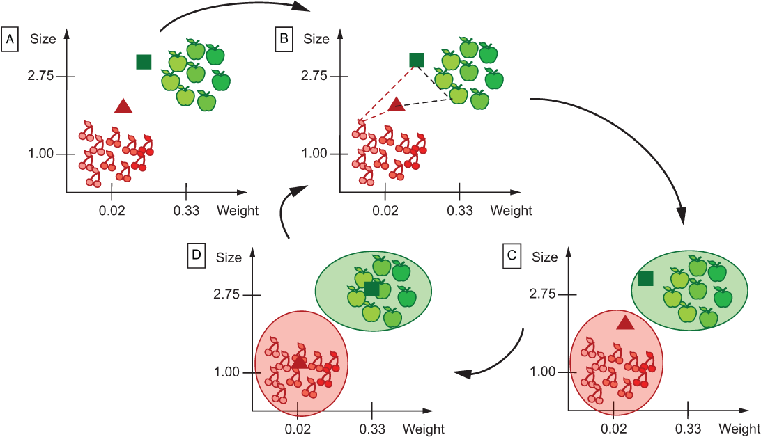
Figure 9.11 Steps of the clustering algorithm: (A) select centroids ® (B) measure distances from each point to each centroid (only some points are visualized here to help readability) ® (C) assign points to clusters ® (D) reestimate centroids. Repeat steps B-D in sequence until the point allocation does not change anymore.

How do you actually calculate the distance between the points? We have discussed Euclidean distance in chapter 1. You first calculate the sum of squared differences between the relevant coordinates of the points, and then take the square root of this sum. Let’s refresh our memory about how it works by trying to solve exercise 9.5 for two dimensions. Note that you can extend this calculation with as many dimensions as you have in your data.

point1=[0.25, 2.31]   point2=[0.05, 1.18]

That’s it! If you are lucky with your original guess of the centroids, your algorithm may find a stable solution (when no point changes its cluster allocation and eventually no centroid moves) quite quickly. This point in the algorithm, when the solution doesn’t change anymore, is called convergence. If there are some tricky cases in your data, whose allocation is hard to establish (perhaps, they bear similarities to both groups and therefore fall somewhere between the clusters), they may flip their membership from one cluster to another over the iterations, thus stopping the algorithm from converging. For such unlucky situations, you need to specify a stopping criterion (e.g., requiring the algorithm to stop after several hundreds of iterations).

Finally, remember that your algorithm is meant to be quite general. You can apply this approach to any fruit basket, and you don’t have to specify which types of fruits are contained in it. Your algorithm is agnostic to the particular clusters it is trying to identify. However, once these clusters are established by the algorithm, you can inspect the characteristics of the centroids and identify what types of fruits are captured by each cluster. For instance, even if we hadn’t visualized the fruits in figures 9.10 and 9.11, you might still be able to tell that a centroid like [color=green, size=avg 2.75 in, weight=avg. 0.33 pounds, shape=round, taste=sweet & sour] is likely to describe an apple or a similar fruit with such characteristics, and [color=red, size=avg 1 in, weight=avg. 0.02 pounds, shape=round, taste=sweet] is likely to describe a cherry (or something similar).

Note This unsupervised algorithm is agnostic not only to the type of clusters it discovers but also to the number of these clusters. The number of clusters that you are looking for in the data is one of the assumptions that you will need to make (e.g., based on some insights, heuristics, or data exploration). For instance, with the number of clusters set to 3, the algorithm might discover [green apples, red apples, cherries] or [apples, large cherries, small cherries], depending on the data at hand.

9.2.2 Clustering for topic discovery

Now that we’ve looked into a toy example of how clustering can be applied to a set of fruits, let’s go back to our Newsgroups posts and see how the same methodology can be applied to a language task. Try answering the questions in exercise 9.6 before moving on.

Let’s apply the unsupervised approach to our data from the 20 Newsgroups dataset. In the previous section, you have already defined a set of posts on the selected 10 categories to work with. You are going to use the same set, only this time you will approach it as if you don’t know what the actual topic labels are. Why is this a good idea? First of all, since you know what the labels in this data actually are, you can evaluate your algorithm at the end. Secondly, you will be able to see what the algorithm identifies in the data by itself, regardless of any assigned labels. After all, it is always possible that someone who posted to one topic actually talked more about another topic. This is exactly what you are going to find out.

First, let’s prepare the data for clustering. Recall that you have already extracted the data from the 20 Newsgroups dataset. There are 5,913 posts in the newsgroups_ train and 3,937 in the newsgroups_test. Since clustering is an unsupervised technique, you don’t have to separate the data into two sets, so let’s combine them together in one set, all_news_data, which should then contain 5,913 + 3,937 = 9,850 posts altogether. You are going to cluster posts based on their content (which you can extract using the dataset.data field); finally, let’s extract the correct labels from the data (recall from the earlier code that they are stored in the dataset.target field) and set them aside. You can use them later to check how the topics discovered in this unsupervised way correspond to the labels originally assigned to the posts. Listing 9.7 walks you through these steps. Recall that it is a good idea to shuffle the data randomly, so let’s import the random functionality and set the seed to a particular value (e.g., 42) to make sure future runs of your code return the same results. Next, the code shows how you can combine the data from newsgroups_train and newsgroups_test into a single list, all_news, mapping the content of each post (accessible via .data) to its label (.target) and using the zip function. After that, you shuffle the tuples and store the contents and labels separately. You will use the contents of the posts in all_news_data for clustering and the actual labels from all_news_labels to evaluate the results. Finally, you should check how many posts you have (length of all_news_data should equal 9,850) and how many unique labels you have using np.unique (the answer should be 10), and take a look into the labels to make sure you have a random shuffle of posts on different topics.

Listing 9.7 Code to prepare the data for clustering

import random
random.seed(42)                                            ❶
 
all_news = list(zip(newsgroups_train.data, newsgroups_train.target))
all_news += list(zip(newsgroups_test.data, 
                     newsgroups_test.target))              ❷
random.shuffle(all_news)                                   ❸
 
all_news_data = [text for (text, label) in all_news]
all_news_labels = [label for (text, label) in all_news]    ❹
 
print("Data:")
print(str(len(all_news_data)) + " posts in "
     + str(np.unique(all_news_labels).shape[0]) 
     + " categories
")                                    ❺
 
print("Labels: ")
print(all_news_labels[:10])
num_clusters = np.unique(all_news_labels).shape[0]
print("Actual number of clusters: " + str(num_clusters))   ❻

❶ To shuffle the data randomly, import the random functionality and set the random seed.

❷ Combine the data from newsgroups_train and newsgroups_test into a single list all_news.

❸ Shuffle the tuples.

❹ Store the contents and labels separately.

❺ Check how many posts and unique labels you have.

❻ Check the labels to make sure you have a random shuffle of posts on different topics.

The preceding code produces the following output:

Data:
9850 posts in 10 categories
 
Labels: 
[2, 6, 1, 9, 0, 5, 1, 2, 9, 0]
Assumed number of clusters: 10

You have 9,850 posts in your data, which cover 10 categories considered before. The printout on labels shows that the posts on different topics are randomly shuffled and that the assumed number of clusters is 10. This is simply what you can assume about this data based on the input (or based on some other insight into the data); however, note that from now on you will approach the task in an unsupervised manner: your algorithm will be working with the 9,850 posts in all_news_data, and it will not get access to the labels contained in all_news_labels, although you can use them at the very last, evaluation, step.

Now that the data is initialized, let’s extract the features. As before, you will use words as features and represent each post as an array, or vector, where each dimension will keep the count or TF-IDF score assigned to the corresponding word—that is, for a particular post, such an array may look like [word₀=0, word₁=5, word₂=0, . . . , word₅₂₇₄₅=3]. To begin with, this looks exactly like the preprocessing and feature extraction steps that you did earlier for the supervised approach. However, this time there are two issues that need to be addressed:

• Remember that to assign data points to clusters, you will need to calculate distances from each data point to each cluster’s centroid. This means calculating differences between the coordinates for 9,850 data points and 10 centroids in 52,746 dimensions, and then comparing the results to detect the closest centroid. Moreover, remember that clustering uses an iterative algorithm, and you will have to perform these calculations repeatedly for, say, 100 iterations. This amounts to a lot of calculations, which will likely make your algorithm very slow.

• In addition, a typical post in this data is relatively short. It might contain a couple of hundreds of words, and assuming that not all of these words are unique (some may be stopwords and some may be repeated several times), the actual word observations for each post will fill in a very small fraction of 52,746 dimensions, filling most of them with zeros. That is, it would be impossible to see any post that will contain a substantial amount of the vocabulary in it and, realistically, every post will have a very small number of dimensions filled with actual occurrence numbers, while the rest will contain zeros. What a waste—not only will you end up with a huge data structure of 9,850 posts by 52,746 word dimensions that will slow your algorithm down, but you will also be using most of this structure for storing zeros. This will make the algorithm very inefficient.

What can be done to address these problems? You’ve come across some solutions to these problems before, while some others will be new for you here:

1. You can ignore stopwords.

2. You can take into account only the words that are contained in a certain number of documents. It would make sense to ignore rare words that occur in less than some minimal number of documents (e.g., 2) or that occur across too many documents (e.g., above 50% of the dataset). You can perform all word-filtering steps in one go using TfidfVectorizer.

3. You can further compress the input data using dimensionality reduction techniques. One widely used technique is singular value decomposition (SVD), which tries to capture the information from the original data matrix with a more compact matrix. This is the technique that we will apply here.

First, let’s look at the code in listing 9.8. In this code, you use TfidfVectorizer to convert text content to vectors, ignoring all words that occur in less that 2 documents (with min_df=2) or in more than 50% of the documents (with max_df=0.5). In addition, you remove stopwords and apply inverse document frequency weights (use_idf=True). Within the transform function, you first transform the original data using a vectorizer and print out the dimensionality of this transformed data. Next, you reduce the number of original dimensions to a much smaller number using TruncatedSVD. TruncatedSVD is particularly suitable for sparse data like the one you are working with here. Then you add TruncatedSVD to a pipeline (make_pipeline from scikit-learn) together with a Normalizer, which helps adjust different ranges of values to the same range, thus helping clustering algorithm’s efficiency. As the output of the transform function, you return both the data with the reduced dimensionality and the svd mapping between the original and the reduced data. Finally, you apply the transformations to all_news_data to compress the original data matrix to a smaller number of features (e.g., 300) and print out the dimensionality of the new data structure.

Listing 9.8 Code to preprocess the data with TfidfVectorizer and SVD

from sklearn.decomposition import TruncatedSVD
from sklearn.pipeline import make_pipeline
from sklearn.preprocessing import Normalizer               ❶
 
vectorizer = TfidfVectorizer(min_df=2, max_df=0.5,         ❷
                            stop_words='english',
                            use_idf=True)                  ❸
 
def transform(data, vectorizer, dimensions):
    trans_data = vectorizer.fit_transform(data)
    print("Transformed data contains: " + str(trans_data.shape[0]) +
          " with " + str(trans_data.shape[1]) 
          + " features =>")                                ❹
 
    svd = TruncatedSVD(dimensions)                         ❺
    pipe = make_pipeline(svd, Normalizer(copy=False))
    reduced_data = pipe.fit_transform(trans_data)          ❻
 
    return reduced_data, svd                               ❼
 
reduced_data, svd = transform(all_news_data, vectorizer, 300)
print("Reduced data contains: " + str(reduced_data.shape[0]) +
     " with " + str(reduced_data.shape[1]) + " features")  ❽

❶ Import all functionality that you are going to use for preprocessing.

❷ Use TfidfVectorizer to convert text content to vectors, ignoring words of certain frequency.

❸ In addition, remove stopwords and apply inverse document frequency weights.

❹ Transform the original data using a vectorizer and print out data dimensionality.

❺ Next, reduce the number of original dimensions to a much smaller number using TruncatedSVD.

❻ Apply a pipeline with a Normalizer.

❼ Return both the data with the reduced dimensionality and the svd mapping.

❽ Apply the transformations to all_news_data to compress the original data matrix.

Here is the output from the code listing:

Transformed data contains: 9850 with 33976 features =>
Reduced data contains: 9850 with 300 features

Let’s now look more closely into this output and make sure all steps make sense. You’ve started out with a huge matrix of 9,850 rows (one per post) and over 50,000 columns (as you know from the supervised ML part, this is how many non-stopwords there are in the training data). This is a lot, and it will make calculations for the clustering algorithm extremely slow. Therefore, you’ve applied two steps in which you successfully reduced the number of columns, as figure 9.12 shows (note that to make the illustration readable, the dimensions are not visualized according to their actual proportions).

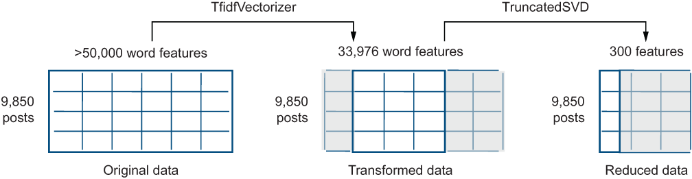
Figure 9.12 Original data dimensionality is reduced using TfidfVectorizer and TruncatedSVD. Grayed areas highlight the bits that are subsequently not considered by the algorithm. First, TfidfVectorizer takes into account only words that occur more frequently than the minimum frequency threshold and less frequently than the maximum frequency threshold. Next, TruncatedSVD identifies the most informative dimensions in the data by compressing the input dimensions to a much more compact representation.

First, you remove all very rare and very frequent words, reducing the number of columns to 33,976, as figure 9.12 shows. Next, the number of considered word columns is severely reduced, from 33,976 to only 300 dimensions, essentially keeping less than 1% of the original dimensions. Let’s look into what is going on under the hood and why such reduction is a justified thing to do to the data.

The goal of the SVD algorithm is to significantly reduce data dimensionality to help expensive algorithms like clustering deal with it more efficiently, while keeping as much of the valuable information in the reduced data as possible. That is, when SVD reduces the data from over 30,000 columns to 300 (thus keeping essentially about 1%), it doesn’t just throw away the other 99% of the data. Instead, it tries to distill and summarize the information contained in the original huge matrix down to a much smaller number of dimensions. How does it achieve that? It relies on the matrix operations from linear algebra (you can read more on SVD, for example, in section 18.2 of https://nlp.stanford.edu/IR-book/pdf/18lsi.pdf). Don’t worry, you don’t need to have deep understanding of the linear algebra operations to use this method; instead let’s get the general overview.

In general, SVD tries to simplify a big matrix representation by decomposing it into three smaller ones in such a way that when you multiply these three smaller matrices, you get back the original one. You can think of this as somewhat similar to decomposing a number like 24 into 4, 3, and 2, as when you multiply these numbers, you get the original number back (i.e., 4 * 3 * 2 = 24). Something similar happens to the big matrix when it gets represented as a product of three smaller ones. Figure 9.13 illustrates this idea.

Figure 9.13 A high-level overview of the truncated singular value decomposition. The original matrix of m rows (texts) and n columns (word features) gets decomposed into three simpler matrices. The first one encodes m texts in terms of a smaller number of k features (concepts, or latent factors); the second one describes the relations of these k concepts to each other; and the third one encodes the relations between the k concepts and the original n word features.

You start with a matrix of 9,850 rows (representing posts) and 33,976 columns (representing words occurring in these posts, that you would like to use as features). That is what the original matrix on the left contains in its m-by-n dimensions (in this case, 9,850 by 33,976). Although you suppose all of these words are useful, as at this point you’ve already filtered out stopwords, very rare words, and very frequent words, this is still too many dimensions to consider, and you might suspect there are ways to extract more useful information from these words and their counts. For instance, consider a set of words like ["car", "cars", "automobile", "automotive"] and so on. These are different words, each with their own dimension (represented with separate columns in the original matrix) and their own counts, yet you might say they are expressing the same concept and, perhaps, there is no point in allocating each of these words separate dimensions. If you had a way to merge the dimensions for all such concept-related words, and instead of working with [word₀, word₁, word₂, . . . , word₃₃₉₇₅], worked with [concept₀, concept₁, concept₂, . . . , concept₂₉₉], this would have simplified your task quite a lot, while keeping all the useful information. This is exactly what SVD is trying to achieve: the matrix of m rows by k columns from figure 9.13 (where the notation k << n means that k is considerably smaller than the original n, as for instance 300 << 33,976) represents the original m (9,850) posts using k (300) concepts, which are also often called latent factors—in other words, factors that are hidden from the naked eye. Let’s visualize this as figure 9.14 does.

Figure 9.14 Application of the truncated SVD algorithm to our data. The original matrix describes the distribution of the original 33,976 words in 9,850 posts. Truncated SVD helps you distill these word features down to 300 most important latent factors. The smaller matrices are more efficient to work with, yet they capture the most important content from the original matrix, and you can always get the original matrix back if you multiply the three component matrices.

The second matrix, k by k (300 by 300), encodes how such latent factors correspond to each other; finally, the third one, k by n (300 by 33,976), tells you how to interpret the relations between the latent factors (or concepts) and the original n words. The beauty of the algorithm is that you can always get back the original m-by-n matrix by multiplying the three smaller matrices, and you don’t need to estimate these constituent matrices yourself; the algorithm does it for you.

What are these k latent factors then and how to select them? These factors are the most prominent (i.e., salient) concepts that the algorithm finds in the data, ordered by their importance, starting with the most prominent one. That is, if you select the first k = 100 factors, you will end up with the most important 100 ones, while k = 300 will add another 200 concepts decreasingly less salient than the first 100 ones. You can continue like that as long as k < n. It is important that the selected number of factors is smaller than the original number of dimensions. There is no ready-made recipe, though, as to how many of such latent factors to consider. This is one of the hyperparameters of the algorithm that you can experiment with. Unfortunately, dimensionality reduction is also one of those useful algorithms that we have to treat as a “black box”: while we can interpret the original 33,976 dimensions and match them to the specific words, all we can say about the reduced space is that dimension₀ corresponds to the most salient concept in the data, dimension₁ to the second most salient one, and so on, but these concepts are no longer represented with specific words. Above, we tried to impose some interpretation on the factors. For instance, we may assume that one of the factors would encode all car-related things. This is a totally reasonable interpretation, but note that the way the algorithm comes up with its “concepts” is based on the word occurrence numbers in the matrix, and what gets combined in the same “concept” is primarily based on the distribution. Despite this lack of interpretability, SVD is a very useful and powerful algorithm, which is why we are using it here.

Now that the data is ready, let’s apply clustering algorithm. Listing 9.9 shows how to do that. Specifically, in this code you use the KMeans clustering algorithm from scikit-learn (see documentation at http://mng.bz/06dE). You apply the algorithm with n_clusters defining the number of clusters to form and centroids to estimate (e.g., you can use 10 here), while k-means++ defines an efficient way to initialize the centroids. The parameter max_iter defines the number of times you iterate through the dataset, and random_state set to a particular value ensures that you get the same results every time you run the algorithm. Finally, you run the algorithm on the reduced_data with the number of clusters equal to 10 (recall that this is the value stored in num_clusters, and it’s based on the number of categories in the input data).

Listing 9.9 Code to run the KMeans clustering algorithm

from sklearn.cluster import KMeans       ❶
 
def cluster(data, num_clusters):
    km = KMeans(n_clusters=num_clusters, 
                init='k-means++',        ❷
                max_iter=100, 
                random_state=0)          ❸
    km.fit(data)
    return km
 
km = cluster(reduced_data, num_clusters) ❹

❶ Import KMeans clustering algorithm from sklearn.

❷ Apply the algorithm with n_clusters defining the number of clusters to form and centroids to estimate.

❸ max_iter defines the number of times you iterate through the dataset.

❹ Run the algorithm on the reduced_data with the number of clusters equal to 10.

The code in this listing performs clustering as discussed earlier in this section. By default, the algorithm runs for up to 100 iterations (or until it converges to a stable solution) with the centroids selected randomly 10 times. Random seed makes sure such random initializations of the centroids can be replicated over multiple runs of your code. Note that here you use an insight about the number of clusters you are looking for: you try to cluster the posts into 10 clusters because you assume, based on the input data, that there are roughly 10 topics here. However, the data may tell you otherwise, and it might turn out that when people post to 10 specific topics, they actually talk about more (or less) than 10 distinct subjects. Therefore, you can change the number of clusters and experiment with other settings.

9.2.3 Evaluation of the topic clustering algorithm

The final step in any algorithm application is evaluation of the results. Let’s see what results you get for the clustering algorithm. Listing 9.10 shows how to evaluate your clustering algorithm’s performance and extract the most informative features. To identify the most informative features, you use the clustering algorithm km and the SVD mapping svd to get back the centroids using svd.inverse_transform on km.cluster_centers_. Then you sort them with argsort and return the matrix with 10 rows (one per cluster) containing the list of most informative dimensions for the cluster centroids, sorted in decreasing order using [:,::-1]. Since the resulting matrix order_centroids contains 10 rows with indices of the most significant words for cluster centroids, you can map them back to words using vectorizer.get_feature_ names() and return, say, 50 per cluster. In the end, you print out the results, as well as the list of category names from the original dataset for reference.

Listing 9.10 Code to evaluate the results obtained with the clustering algorithm

def evaluate(km, labels, svd):
    print("Clustering report:
")
    print(
        f"* Homogeneity: {str(metrics.homogeneity_score(labels, km.labels_))}"
        )
    print(
        f"* Completeness: {str(metrics.completeness_score(labels, km.labels_))}"
        )
    print(
        f"* V-measure: {str(metrics.v_measure_score(labels, km.labels_))}"
        )                                                     ❶
 
    print("
Most discriminative words per cluster:")
    original_space_centroids = svd.inverse_transform(
        km.cluster_centers_)                                  ❷
    order_centroids = 
             original_space_centroids.argsort()[:, ::-1]      ❸
 
    terms = vectorizer.get_feature_names()
    for i in range(num_clusters):
        print("Cluster " + str(i) + ": ")
        cl_terms = ""
        for ind in order_centroids[i, :50]:
            cl_terms += terms[ind] + " "
        print(cl_terms + "
")                               ❹
 
evaluate(km, all_news_labels, svd)
 
print("
Categories:")
for i, category in enumerate(newsgroups_train.target_names):
    print("*", category)                                     ❺

❶ Report the clustering evaluation metrics.

❷ Get back the centroids using svd.inverse_transform on km.cluster_centers_.

❸ Sort them and return the matrix containing the list of most informative dimensions for the cluster centroids.

❹ Map them back to words using vectorizer.get_feature_names() and return 50 per cluster.

❺ Print the list of category names from the original dataset for reference.

This code returns the following output ([...] is used to truncate the output for space reasons):

Clustering report:
 
* Homogeneity: 0.4905834160659784
* Completeness: 0.5545553250427578
* V-measure: 0.5206115419058042
 
Most discriminative words per cluster:
Cluster 0: 
key chip encryption government keys nsa algorithm secure security encrypted [...]
 
Cluster 1: 
doctor disease medical patients pain cause cancer treatment drug body [...]
 
Cluster 2: 
game team hockey players season play win baseball league nhl [...]
 
Cluster 3: 
just don like think know people does good right say [...]
 
Cluster 4: 
window server widget display application file windows program running code [...]
 
Cluster 5: 
sale offer shipping condition asking new drive sell interested price [...]
 
Cluster 6: 
car bike engine cars miles ride rear speed oil road [...]
 
Cluster 7: 
thanks mail advance know address send list email edu information [...] 
 
Cluster 8: 
space orbit launch nasa shuttle moon earth mission lunar solar [...] 
 
Cluster 9: 
israel jews israeli armenian arab people jewish armenians turkish war [...]
 
 
Categories:
* comp.windows.x
[...]

The metrics used here try to mirror the metrics you used for supervised ML:

• Homogeneity—Measures to what extent each cluster contains only members of a single class (to a certain extent, this metric is similar to precision). For example, does cluster₀ contain posts only on cryptography, and cluster₁ posts only on medicine, and so on?

• Completeness —Measures whether members of a single category end up in the same cluster. For instance, have all cryptography posts ended up in cluster₀ and all medicine-related posts ended up in cluster₁, and so on? This is, to some extent, similar to recall.

• V-measure—Equivalent to F-measure in the unsupervised context, as it also represents a harmonic mean between the other two metrics.

The precise calculations for these metrics are different from those for precision, recall, and F-measure in a supervised ML setting, and the two sets of values are not directly comparable. The metrics here should be interpreted in the following way: each score lies in the range of [0, 1], with perfect assignment of posts to clusters getting scores of 1 (as in this case each topic is represented with a single cluster, and each cluster contains posts only from a single topic) and the mixed up clusters resulting in scores of 0. Thus, the closer the scores are to 1, the better the clusters identified by the algorithm. The scores that you are getting here (homogeneity of 0.49 and completeness of 0.55) show that the clusters are not perfect and there is a fair number of posts from different topics being grouped in a single cluster as well as posts from the same topic being split across several clusters.

Note Unsupervised measures rely on the estimation of entropy rather than simple proportions. For more details, check the original paper at www.aclweb.org/anthology/D07-1043.pdf, and for examples, take a look at scikit-learn’s documentation at http://mng.bz/Kxqg.

To find out more about the precise assignment of posts to clusters, let’s try to further interpret the results from listing 9.10 looking at each cluster, as exercise 9.7 suggests.

Let’s look into the solution together. Table 9.6 presents possible interpretations.

Table 9.6 Possible topic allocations for the identified clusters

As you can see, the unsupervised method uncovered some new insights into the data. You’ve started with the assumption that the 10 topics will clearly express themselves in the word choice, thus setting the number of clusters to 10. As a result, you’ve identified 10 clusters, some of which (like clusters 2 and 6) may combine posts on closely related topics (e.g., baseball & hockey, or autos & motorcycles), whereas other topics may end up being spread across multiple clusters (e.g., forsale seems to be a very heterogeneous topic—put under misc, or miscellaneous—and it’s probably no wonder that it gets allocated 2 or potentially 3 different clusters).

This difference in the labels from our dataset and the groups identified by the clustering algorithm on the basis of the data itself is the main reason for homogeneity and completeness scores not being equal to 1.0. Since the main goal of unsupervised approaches is to get new insights into the data, this is not necessarily a bad result. It suggests that the posts on some topics may be merged under one heading (e.g., on your news platform, you may consider putting all posts on baseball & hockey on the same page called Sports), while posts from some other topics that you may have assumed to be homogeneous should actually be split into several subgroups (e.g., you may consider creating multiple subtopics for selling different items).

As a final remark, we said before that the clustering algorithm is agnostic to the set of topics that it is trying to discover. It can group posts on the same topic into a single cluster and provide you with the informative words, but it won’t be able to automatically assign the label for the identified topic (i.e., without further help, it won’t be able to solve exercise 9.7 as you just did). Is there a way to automatically assign topic labels to the identified clusters, then? The solution is to combine supervised and unsupervised approaches. A widely used scenario for clustering is when you have a small amount of labeled data and a large amount of unlabeled data, in which case you can use clustering to identify similar posts (both among labeled and unlabeled ones) and assign the label based on the allocation of the labeled posts from the correspondent clusters. Alternatively, you can try to automatically generate topic labels based on the set of informative words returned by the clustering algorithm.

Summary

• There are two different paradigms within which you can analyze topics, supervised and unsupervised.

• If you have texts labeled with topics, you can apply a supervised machine learning algorithm. By now, you are quite familiar with this family of algorithms, but the novelty in topic classification is that you need to extend the task to a multiclass setting.

• A machine-learning pipeline can be applied to this task, making use of the 20 Newsgroups dataset available via scikit-learn, selecting words as features, applying TF-IDF transformations to the raw word counts, and using multinomial Naïve Bayes algorithm from the scikit-learn suite.

• Additive smoothing is a technique that is widely used in classification with probabilistic algorithms, and that helps address data effects. Note that if you haven’t seen a particular word in texts on a particular topic, you should assume that you don’t have enough training data (which is always the most realistic assumption) rather than that this word is absolutely impossible to use with the specific topic. Smoothing helps adjust the probabilities, giving previously unseen words a small chance of occurrence in the future.

• When you don’t have labeled data or you want to discover the topics from the data itself, you can use an unsupervised ML approach.

• K-means clustering algorithm can be applied to learn how the topics are represented in the data. This approach clusters similar texts based on word occurrences. In doing so, it identifies the representative central points for each cluster, called centroids. K in this algorithm represents the number of clusters (and centroids); for example, k = 10. K-means is an iterative algorithm that runs either for a predefined number of steps or until convergence (i.e., until a stable solution is found, and the data points don’t change their cluster membership anymore).

• To estimate the centroids and find clusters, the algorithm needs to calculate distances in a multidimensional space, such as by using Euclidean distance. The number of dimensions is defined by the number of considered features. In this task, it is the words. To reduce the dimensionality of the word space, a number of familiar techniques can be used, including stopwords removal and removal of very rare and very frequent words with TfidfVectorizer.

• Truncated singular value decomposition is a useful technique that allows you to distill the information contained in the original vector dimensions down to a much smaller number of informative dimensions, thus making calculations much more efficient. This technique essentially allows you to convert original words into concepts (also called latent factors).

• Clustering algorithms can be evaluated using homogeneity (an alternative for precision in the unsupervised ML setting), completeness (alternative to recall), and V-measure (alternative to F-score). In addition, the informative words that helped the clustering algorithm identify each cluster’s centroid can be extracted and analyzed. Based on these words, you can interpret the results. For instance, you can reason about the clusters identified in the data and how they correspond to the labeled topics.

• When you want to identify topics present in the data and investigate how they are distributed across the documents, which words represent each topic and to what extent, you can use another unsupervised approach—topic modeling. This will be the subject of the next chapter.

Solutions to miscellaneous exercises

Exercise 9.1

1. Previous tasks explored various types of features. Recall that in chapter 6 you did quite an extensive feature exploration for authorship identification and used features as diverse as word and sentence lengths, count and proportion of stopwords, distributions of parts of speech and word suffixes, and the presence of unique words. For sentiment analysis in chapters 7 and 8, you mostly relied on words, but recall that this also required some selection of features. For instance, you filtered out words using sentiment lexicons, considered the effect that negative words have on the rest of the text, and used n-grams that cover sequences of n words.

2. Feature selection heavily depends on the task at hand. For instance, the distribution of stopwords and word suffixes, the presence of some unique words, or sentence length may be very characteristic of a particular author’s writing style. Note that the 20 Newsgroups dataset (like many other collections of texts) are written by a wide variety of authors, and even if some authors prefer to write on specific topics, identification of writing styles is peripheral to the task of topic detection. This means that such fine-grained features as unique words or distribution of suffixes and stopwords are unlikely to be helpful. It is also unlikely that different topics would vary significantly in terms of the sentence and word lengths. Although such features may help distinguish between texts of different genres (e.g., social media posts are typically shorter than scientific articles) within the Newsgroups posts, these features would probably not be very helpful. Among all the tasks addressed so far in this book, topic classification is most similar to spam detection (e.g., although it is possible that ham emails talk about “lotteries” and “medication,” too, one would expect to see such words in spam emails more frequently). Words and their distributions are the most reliable feature type for topic classification too. For instance, one would expect to see a word like car much more frequently in rec.autos posts on automobiles than in sci.med posts on medicine, and a word like virus in sci.med, comp.windows.x, and, perhaps, sci.crypt (cryptography) posts but not so much in misc.forsale (sale announcements).

Exercise 9.2

A collection of words in (1) would strongly suggest a rec.autos topic (automobiles), while the set in (2) most likely refers to sci.space.

Exercise 9.3

In this book, you have come across a number of evaluation metrics in the previous tasks you worked on. Among them are

• Accuracy—The proportion of correctly classified examples among those that you tried to classify

• Precision—The proportion of texts that actually belong to the topic among those that your algorithm identifies as belonging to the topic

• Recall—The proportion of texts that are correctly identified as belonging to the topic among those that actually belong to this topic

• F-score—The harmonic mean between the precision and recall scores

Exercise 9.4

The comparatively low recall of 0.78 on rec.autos posts means that some posts from this topic are misclassified as other categories. This follows directly from the recall definition:

Recall = number of texts from rec.auto classified as rec.auto / 
         number of texts that are actually in rec.auto

This means that the proportion of texts from rec.auto identified by the classifier is 0.78, suggesting that the other texts are incorrectly assigned with other categories by the classifier. The relatively low precision of 0.71 on rec.sport.hockey suggests that some of the texts that the classifier believes are related to hockey are actually from other categories. This follows from the precision definition:

Precision = number of texts from rec.sport.hockey classified as rec.sport.hockey / 
            number of texts classified as rec.sport.hockey

This suggests that the proportion of texts that are classified as rec.sport.hockey and that are actually from this category equals 0.71, with the rest of the texts classified with this category actually belonging to some other categories. Perhaps, even to rec.auto. Listing 9.6 helps you find this out.

Exercise 9.5

Let’s estimate the distances first (note, sqrt is used for square root):

dist(point1, centroid1) = sqrt ((0.25-0.33)2 + (2.31-2.75)2)= sqrt (0.2000)=0.45
dist(point1, centroid2) = sqrt ((0.25-0.02)2 + (2.31-1.00)2)= sqrt (1.7690)=1.33
dist(point2, centroid1) = sqrt ((0.05-0.33)2 + (1.18-2.75)2)= sqrt (2.5433)=1.60
dist(point2, centroid2) = sqrt ((0.05-0.02)2 + (1.18-1.00)2)= sqrt (0.0333)=0.18

These estimations show that point₁ is closer to centroid₁ (0.45 versus 1.33), so it belongs in cluster₁; point₂ is closer to centroid₂ (0.18 versus 1.60), so it belongs in cluster₂. Figure 9.15 visualizes these calculations and provides you with the general formula for Euclidean distance.

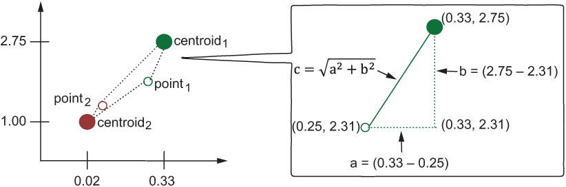
Figure 9.15 A reminder of how Euclidean distance is calculated. This graph shows two selected points and two centroids, and explains how the distance is calculated, zooming in on centroid₁ and point₁, and showing the calculation steps.

Exercise 9.6

Your “fruit basket” this time is the collection of posts from the 20 Newsgroups dataset. The goal of unsupervised approaches is to discover groups of similar objects (in this case, posts) in the data based on some characteristics that can help the algorithm tell different objects apart and combine similar objects in relatively homogeneous clusters. Here, you are trying to discover topics based on the content of the posts. Therefore, your clusters will represent topics, and each point will represent a separate post. You can use the vocabulary of the words identified by the algorithm in the training data (the set of 52,746 words as before) as coordinates in space. That is, instead of [color=green, size=avg. 2.75 in, weight=avg. 0.33 pounds, shape=round, taste= sweet & sour], you will be using something like [word₀=0, word₁=5, word₂=0,..., word₅₂₇₄₅=3], where values represent either the absolute number of occurrences of a particular word in text or their TF-IDF scores. Note that this means that, unlike in our toy example, where you represented each point in a five-dimensional space, in a language task you may be dealing with thousands of dimensions.