
CHAPTER 21
Advanced Static Analysis with IDA Pro
In this chapter, you will be introduced to additional features of IDA Pro that will help you analyze binary code more efficiently and with greater confidence. Out of the box, IDA Pro is already one of the most powerful binary analysis tools available. The range of processors and binary file formats that IDA Pro can process is more than many users will ever need. Likewise, the disassembly view provides all of the capability that the majority of users will ever want. Occasionally, however, a binary will be sufficiently sophisticated or complex that you will need to take advantage of IDA Pro’s advanced features to fully comprehend what the binary does. In other cases, you may find that IDA Pro does a large percentage of what you wish to do, and you would like to pick up from there with additional automated processing. Thus, in this chapter, we examine the following major topics:
• Static analysis challenges
• Extending IDA Pro
Static Analysis Challenges
For any nontrivial binary, generally several challenges must be overcome to make analysis of that binary less difficult. Examples of challenges you might encounter include
• Binaries that have been stripped of some or all of their symbol information
• Binaries that have been linked with static libraries
• Binaries that make use of complex, user-defined data structures
• Compiled C++ programs that make use of polymorphism
• Binaries that have been obfuscated in some manner to hinder analysis
• Binaries that use instruction sets with which IDA Pro is not familiar
• Binaries that use file formats with which IDA Pro is not familiar
IDA Pro is equipped to deal with all of these challenges to varying degrees, though its documentation may not indicate that. One of the first things you need to learn to accept as an IDA Pro user is that there is no user’s manual and the help files are pretty terse. Familiarize yourself with the available online IDA Pro resources as, aside from your own hunting around and poking at IDA Pro, they will be your primary means of answering questions. Some sites that have strong communities of IDA Pro users include OpenRCE (www.openrce.org), Hex Blog (www.hexblog.com), and the IDA Pro support boards at the Hex-Rays website (see the “References” section at the end of the chapter for more details).
Stripped Binaries
The process of building software generally consists of several phases. In a typical C/C++ environment, you will encounter at a minimum the preprocessor, compilation, and linking phases before an executable can be produced. For follow-on phases to correctly combine the results of previous phases, intermediate files often contain information specific to the next build phase. For example, the compiler embeds into object files a lot of information that is specifically designed to assist the linker in doing its job of combining those object files into a single executable or library. Among other things, this information includes the names of all the functions and global variables within the object file. Once the linker has done its job, however, this information is no longer necessary. Quite frequently, all of this information is carried forward by the linker and remains present in the final executable file, where it can be examined by tools such as IDA Pro to learn what all the functions within a program were originally named. If we assume, which can be dangerous, that programmers tend to name functions and variables according to their purpose, then we can learn a tremendous amount of information simply by having these symbol names available to us.
The process of “stripping” a binary involves removing all symbol information that is no longer required once the binary has been built. Stripping is generally performed by using the command-line strip utility and, as a result of removing extraneous information, has the side effect of yielding a smaller binary. From a reverse-engineering perspective, however, stripping makes a binary slightly more difficult to analyze as a result of the loss of all the symbols. In this regard, stripping a binary can be seen as a primitive form of obfuscation. The most immediate impact of dealing with a stripped binary in IDA Pro is that IDA Pro will be unable to locate the main() function and will instead initially position the disassembly view at the program’s true entry point, generally named _start.

NOTE
Contrary to popular belief, main is not the first thing executed in a compiled C or C++ program. A significant amount of initialization must take place before control can be transferred to main. Some of the startup tasks include initialization of the C libraries, initialization of global objects, and creation of the argv and envp arguments expected by main.
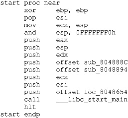
You will seldom desire to reverse-engineer all of the startup code added by the compiler, so locating main is a handy thing to be able to do. Fortunately, each compiler tends to have its own style of initialization code, so with practice you will be able to recognize the compiler that was used based simply on the startup sequence. Since the last thing that the startup sequence does is transfer control to main, you should be able to locate main easily regardless of whether a binary has been stripped. Listing 21-1 shows the _start function for a gcc-compiled binary that has not been stripped.
Listing 21-1

Notice that main is not called directly; rather, it is passed as a parameter to the library function __libc_start_main. The __libc_start_main function takes care of libc initialization, pushing the proper arguments to main, and finally transferring control to main. Note that main is the last parameter pushed before the call to __libc_start_main. Listing 21-2 shows the _start function from the same binary after it has been stripped.
Listing 21-2
In this second case, we can see that IDA Pro no longer understands the name main. We also notice that two other function names have been lost as a result of the stripping operation, while one function has managed to retain its name. It is important to note that the behavior of _start has not been changed in any way by the stripping operation. As a result, we can apply what we learned from Listing 21-1, that main is the last argument pushed to __libc_start_main, and deduce that loc_8046854 must be the start address of main; we are free to rename loc_8046854 to main as an early step in our reversing process.
One question we need to understand the answer to is why __libc_start_main has managed to retain its name while all the other functions we saw in Listing 21-1 lost theirs. The answer lies in the fact that the binary we are looking at was dynamically linked (the file command would tell us so) and __libc_start_main is being imported from libc.so, the shared C library. The stripping process has no effect on imported or exported function and symbol names. This is because the runtime dynamic linker must be able to resolve these names across the various shared components required by the program. We will see in the next section that we are not always so lucky when we encounter statically linked binaries.
Statically Linked Programs and FLAIR
When compiling programs that make use of library functions, the linker must be told whether to use shared libraries such as .dll or .so files, or static libraries such as .a files. Programs that use shared libraries are said to be dynamically linked, while programs that use static libraries are said to be statically linked. Each form of linking has its own advantages and disadvantages. Dynamic linking results in smaller executables and easier upgrading of library components at the expense of some extra overhead when launching the binary, and the chance that the binary will not run if any required libraries are missing. To learn which dynamic libraries an executable depends on, you can use the dumpbin utility on Windows, ldd on Linux, and otool on Mac OS X. Each will list the names of the shared libraries that the loader must find in order to execute a given dynamically linked program. Static linking results in much larger binaries because library code is merged with program code to create a single executable file that has no external dependencies, making the binary easier to distribute. As an example, consider a program that makes use of the OpenSSL cryptographic libraries. If this program is built to use shared libraries, then each computer on which the program is installed must contain a copy of the OpenSSL libraries. The program would fail to execute on any computer that does not have OpenSSL installed. Statically linking that same program eliminates the requirement to have OpenSSL present on computers that will be used to run the program, making distribution of the program somewhat easier.
From a reverse-engineering point of view, dynamically linked binaries are somewhat easier to analyze, for several reasons. First, dynamically linked binaries contain little to no library code, which means that the code that you get to see in IDA Pro is just the code that is specific to the application, making it both smaller and easier to focus on application-specific code rather than library code. The last thing you want to do is spend your time reversing library code that is generally accepted to be fairly secure. Second, when a dynamically linked binary is stripped, it is not possible to strip the names of library functions called by the binary, which means the disassembly will continue to contain useful function names in many cases. Statically linked binaries present more of a challenge because they contain far more code to disassemble, most of which belongs to libraries. However, as long as the statically linked program has not been stripped, you will continue to see all the same names that you would see in a dynamically linked version of the same program. A stripped, statically linked binary presents the largest challenge for reverse engineering. When the strip utility removes symbol information from a statically linked program, it removes not only the function and global variable names associated with the program, but also the function and global variable names associated with any libraries that were linked in. As a result, it is extremely difficult to distinguish program code from library code in such a binary. Further, it is difficult to determine exactly how many libraries may have been linked into the program. IDA Pro has facilities (not well documented) for dealing with exactly this situation.
Listing 21-3 shows what our _start function ends up looking like in a statically linked, stripped binary.
Listing 21-3
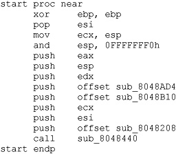
At this point, we have lost the names of every function in the binary and we need some method for locating the main function so that we can begin analyzing the program in earnest. Based on what we saw in Listings 21-1 and 21-2, we can proceed as follows:
• Find the last function called from _start; this should be __libc_start_main.
• Locate the first argument to __libc_start_main; this will be the topmost item on the stack, usually the last item pushed prior to the function call. In this case, we deduce that main must be sub_8048208. We are now prepared to start analyzing the program beginning with main.
Locating main is only a small victory, however. By comparing Listing 21-4 from the unstripped version of the binary with Listing 21-5 from the stripped version, we can see that we have completely lost the ability to distinguish the boundaries between user code and library code.
Listing 21-4

Listing 21-5

In Listing 21-5, we have lost the names of stderr, fwrite, exit, and gethostbyname, and each is indistinguishable from any other user space function or global variable. The danger we face is that, being presented with the binary from Listing 21-5, we might attempt to reverse-engineer the function at loc_8048F7C. Having done so, we would be disappointed to learn that we have done nothing more than reverse a piece of the C standard library. Clearly, this is not a desirable situation for us. Fortunately, IDA Pro possesses the ability to help out in these circumstances.
Fast Library Identification and Recognition Technology (FLIRT) is the name that IDA Pro gives to its ability to automatically recognize functions based on pattern/signature matching. IDA Pro uses FLIRT to match code sequences against many signatures for widely used libraries. IDA Pro’s initial use of FLIRT against any binary is to attempt to determine the compiler that was used to generate the binary. This is accomplished by matching entry point sequences (such as those we saw in Listings 21-1 through 21-3) against stored signatures for various compilers. Once the compiler has been identified, IDA Pro attempts to match against additional signatures more relevant to the identified compiler. In cases where IDA Pro does not pick up on the exact compiler that was used to create the binary, you can force IDA Pro to apply any additional signatures from IDA Pro’s list of available signature files. Signature application takes place via the File | Load File | FLIRT Signature File menu option, which brings up the dialog box shown in Figure 21-1.

Figure 21-1 IDA Pro library signature selection dialog box
The dialog box is populated based on the contents of IDA Pro’s sig subdirectory. Selecting one of the available signature sets causes IDA Pro to scan the current binary for possible matches. For each match that is found, IDA Pro renames the matching code in accordance with the signature. When the signature files are correct for the current binary, this operation has the effect of unstripping the binary. It is important to understand that IDA Pro does not come complete with signatures for every static library in existence. Consider the number of different libraries shipped with any Linux distribution and you can appreciate the magnitude of this problem. To address this limitation, Hex-Rays ships a tool set called Fast Library Acquisition for Identification and Recognition (FLAIR). FLAIR consists of several command-line utilities used to parse static libraries and generate IDA Pro-compatible signature files.
Generating IDA Pro Sig Files
Installation of the FLAIR tools is as simple as unzipping the FLAIR distribution (flair51.zip used in this section) into a working directory. Beware that FLAIR distributions are generally not backward compatible with older versions of IDA Pro, so be sure to obtain the appropriate version of FLAIR for your version of IDA Pro from the Hex-Rays IDA Pro Downloads page (see “References”). After you have extracted the tools, you will find the entire body of existing FLAIR documentation in the three files named pat.txt, readme.txt, and sigmake.txt. You are encouraged to read through these files for more detailed information on creating your own signature files.
The first step in creating signatures for a new library involves the extraction of patterns for each function in the library. FLAIR comes with pattern-generating parsers for several common static library file formats. All FLAIR tools are located in FLAIR’s bin subdirectory. The pattern generators are named pXXX, where XXX represents various library file formats. In the following example, we will generate a sig file for the statically linked version of the standard C library (libc.a) that ships with FreeBSD 6.2. After moving libc.a onto our development system, the following command is used to generate a pattern file:
# ./pelf libc.a libc_FreeBSD62.pat
libc_FreeBSD62.a: skipped 0, total 988
We choose the pelf tool because FreeBSD uses ELF format binaries. In this case, we are working in FLAIR’s bin directory. If you wish to work in another directory, the usual PATH issues apply for locating the pelf program. FLAIR pattern files are ASCII text files containing patterns for each exported function within the library being parsed. Patterns are generated from the first 32 bytes of a function, from some intermediate bytes of the function for which a CRC16 value is computed, and from the 32 bytes following the bytes used to compute the cyclic redundancy check (CRC). Pattern formats are described in more detail in the pat.txt file included with FLAIR. The second step in creating a sig file is to use the sigmake tool to create a binary signature file from a generated pattern file. The following command attempts to generate a sig file from the previously generated pattern file:
# ../sigmake.exe -n"FreeBSD 6.2 standard C library"
> libc_FreeBSD62.pat libc_FreeBSD62.sig
See the documentation to learn how to resolve collisitions.
: modules/leaves: 13443664/988, COLLISIONS: 924
The –n option can be used to specify the “Library name” of the sig file as displayed in the sig file selection dialog box (see Figure 21-1). The default name assigned by sig make is “Unnamed Sample Library.” The last two arguments for sigmake represent the input pattern file and the output sig file, respectively. In this example, we seem to have a problem: sigmake is reporting some collisions. In a nutshell, collisions occur when two functions reduce to the same signature. If any collisions are found, sigmake refuses to generate a sig file and instead generates an exclusions (.exc) file. The first few lines of this particular exclusions file are shown here:
;--------- (delete these lines to allow sigmake to read this file)
; add '+' at the start of a line to select a module
; add '-' if you are not sure about the selection
; do nothing if you want to exclude all modules
___ntohs 00 0000 FB744240486C4C3................................................
___htons 00 0000 FB744240486C4C3................................................
In this example, we see that the functions ntohs and htons have the same signature, which is not surprising considering that they do the same thing on an x86 architecture, namely swap the bytes in a 2-byte short value. The exclusions file must be edited to instruct sigmake how to resolve each collision. As shown earlier, basic instructions for this can be found in the generated .exc file. At a minimum, the comment lines (those beginning with a semicolon) must be removed. You must then choose which, if any, of the colliding functions you wish to keep. In this example, if we choose to keep htons, we must prefix the htons line with a + character, which tells sigmake to treat any function with the same signature as if it were htons rather than ntohs. More detailed instructions on how to resolve collisions can be found in FLAIR’s sigmake.txt file. Once you have edited the exclusions file, simply rerun sigmake with the same options. A successful run will result in no error or warning messages and the creation of the requested sig file. Installing the newly created signature file is simply a matter of copying it to the sig subdirectory under your main IDA Pro program directory. The installed signatures will now be available for use, as shown in Figure 21-2.
Applying the new signatures to the following code:

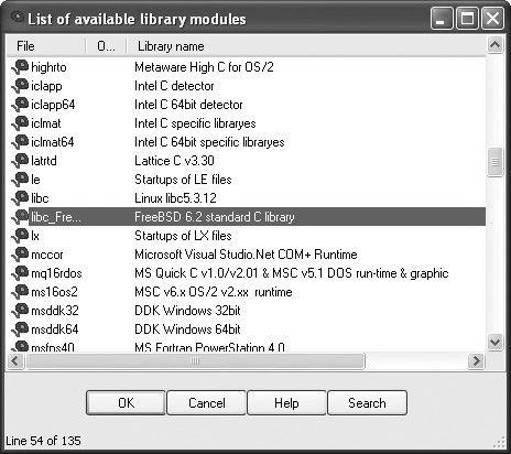
Figure 21-2 Selecting appropriate signatures
yields the following improved disassembly in which we are far less likely to waste time analyzing any of the three functions that are called:

We have not covered how to identify exactly which static library files to use when generating your IDA Pro sig files. It is safe to assume that statically linked C programs are linked against the static C library. To generate accurate signatures, it is important to track down a version of the library that closely matches the one with which the binary was linked. Here, some file and strings analysis can assist in narrowing the field of operating systems that the binary may have been compiled on. The file utility can distinguish among various platforms such as Linux, FreeBSD, and Mac OS X, and the strings utility can be used to search for version strings that may point to the compiler or libc version that was used. Armed with that information, you can attempt to locate the appropriate libraries from a matching system. If the binary was linked with more than one static library, additional strings analysis may be required to identify each additional library. Useful things to look for in strings output include copyright notices, version strings, usage instructions, or other unique messages that could be thrown into a search engine in an attempt to identify each additional library. By identifying as many libraries as possible and applying their signatures, you greatly reduce the amount of code that you need to spend time analyzing and get to focus more attention on application-specific code.
Data Structure Analysis
One consequence of compilation being a lossy operation is that we lose access to data declarations and structure definitions, which makes it far more difficult to understand the memory layout in disassembled code. As mentioned in Chapter 20, IDA Pro provides the capability to define the layout of data structures and then to apply those structure definitions to regions of memory. Once a structure template has been applied to a region of memory, IDA Pro can utilize structure field names in place of integer offsets within the disassembly, making the disassembly far more readable. There are two important steps in determining the layout of data structures in compiled code. The first step is to determine the size of the data structure. The second step is to determine how the structure is subdivided into fields and what type is associated with each field. The program in Listing 21-6 and its corresponding compiled version in Listing 21-7 will be used to illustrate several points about disassembling structures.
Listing 21-6
1: #include <stdlib.h>
2: #include <math.h>
3: #include <string.h>
4: typedef struct GrayHat_t {
5: char buf[80];
6: int val;
7: double squareRoot;
8: } GrayHat;
9: int main(int argc, char **argv) {
10: GrayHat gh;
11: if (argc == 4) {
12: GrayHat *g = (GrayHat*)malloc(sizeof(GrayHat));
13: strncpy(g->buf, argv[1], 80);
14: g->val = atoi(argv[2]);
15: g->squareRoot = sqrt(atof(argv[3]));
16: strncpy(gh.buf, argv[0], 80);
17: gh.val = 0xdeadbeef;
18: }
19: return 0;
20: }
Listing 21-7
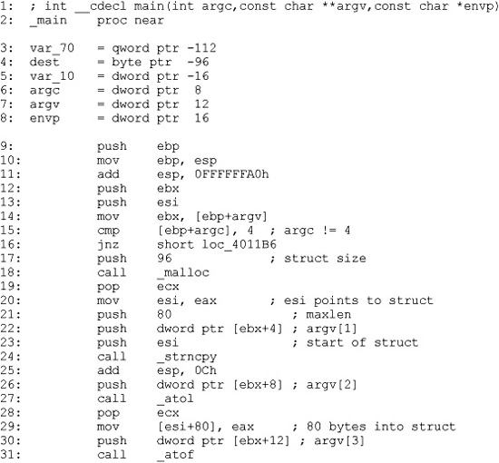
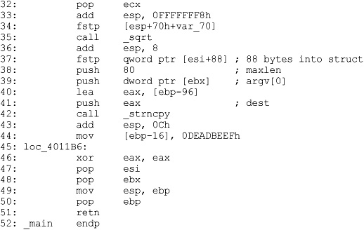
There are two methods for determining the size of a structure. The first and easiest method is to find locations at which a structure is dynamically allocated using malloc or new. Lines 17 and 18 in Listing 21-7 show a call to malloc 96 bytes of memory. Malloced blocks of memory generally represent either structures or arrays. In this case, we learn that this program manipulates a structure whose size is 96 bytes. The resulting pointer is transferred into the esi register and used to access the fields in the structure for the remainder of the function. References to this structure take place at lines 23, 29, and 37.
The second method of determining the size of a structure is to observe the offsets used in every reference to the structure and to compute the maximum size required to house the data that is referenced. In this case, line 23 references the 80 bytes at the beginning of the structure (based on the maxlen argument pushed at line 21), line 29 references 4 bytes (the size of eax) starting at offset 80 into the structure ([esi + 80]), and line 37 references 8 bytes (a quad word/qword) starting at offset 88 ([esi + 88]) into the structure. Based on these references, we can deduce that the structure is 88 (the maximum offset we observe) plus 8 (the size of data accessed at that offset), or 96 bytes long. Thus we have derived the size of the structure by two different methods. The second method is useful in cases where we can’t directly observe the allocation of the structure, perhaps because it takes place within library code.
To understand the layout of the bytes within a structure, we must determine the types of data that are used at each observable offset within the structure. In our example, the access at line 23 uses the beginning of the structure as the destination of a string copy operation, limited in size to 80 bytes. We can conclude therefore that the first 80 bytes of the structure is an array of characters. At line 29, the 4 bytes at offset 80 in the structure are assigned the result of the function atol, which converts an ASCII string to a long value. Here we can conclude that the second field in the structure is a 4-byte long. Finally, at line 37, the 8 bytes at offset 88 into the structure are assigned the result of the function atof, which converts an ASCII string to a floating-point double value.
You may have noticed that the bytes at offsets 84–87 of the structure appear to be unused. There are two possible explanations for this. The first is that there is a structure field between the long and the double that is simply not referenced by the function. The second possibility is that the compiler has inserted some padding bytes to achieve some desired field alignment. Based on the actual definition of the structure in Listing 21-6, we conclude that padding is the culprit in this particular case. If we wanted to see meaningful field names associated with each structure access, we could define a structure in the IDA Pro Structures window, as described in Chapter 20. IDA Pro offers an alternative method for defining structures that you may find far easier to use than its structure editing facilities. IDA Pro can parse C header files via the File | Load File menu option. If you have access to the source code or prefer to create a C-style struct definition using a text editor, IDA Pro will parse the header file and automatically create structures for each struct definition that it encounters in the header file. The only restriction you must be aware of is that IDA Pro only recognizes standard C data types. For any nonstandard types, uint32_t, for example, the header file must contain an appropriate typedef, or you must edit the header file to convert all nonstandard types to standard types.
Access to stack or globally allocated structures looks quite different from access to dynamically allocated structures. Listing 21-6 shows that main contains a local, stack allocated structure declared at line 10. Lines 16 and 17 of main reference fields in this local structure. These correspond to lines 40 and 44 in the assembly Listing 21-7. While we can see that line 44 references memory that is 80 bytes ([ebp-96+80] == [ebp-16]) after the reference at line 40, we don’t get a sense that the two references belong to the same structure. This is because the compiler can compute the address of each field (as an absolute address in a global variable, or a relative address within a stack frame) at compile time, whereas access to fields in dynamically allocated structures must always be computed at runtime because the base address of the structure is not known at compile time.
Using IDA Pro Structures to View Program Headers
In addition to enabling you to declare your own data structures, IDA Pro contains a large number of common data structure templates for various build environments, including standard C library structures and Windows API structures. An interesting example use of these predefined structures is to use them to examine the program file headers which, by default, are not loaded into the analysis database. To examine file headers, you must perform a manual load when initially opening a file for analysis. Manual loads are selected via a checkbox on the initial load dialog box, as shown in Figure 21-3.
Manual loading forces IDA Pro to ask you whether you wish to load each section of the binary into IDA Pro’s database. One of the sections that IDA Pro will ask about is the header section, which will allow you to see all the fields of the program headers, including structures such as the MSDOS and NT file headers. Another section that gets loaded only when a manual load is performed is the resource section that is used on the Windows platform to store dialog box and menu templates, string tables, icons, and the file properties. You can view the fields of the MSDOS header by scrolling to the beginning of a manually loaded Windows PE file and placing the cursor on the first address in the database, which should contain the ‘M’ value of the MSDOS ‘MZ’ signature. No layout information will be displayed until you add the IMAGE_DOS_HEADER to your Structures window. This is accomplished by switching to the Structures tab, clicking Insert, entering IMAGE_DOS_HEADER as the Structure Name, as shown in Figure 21-4, and clicking OK.
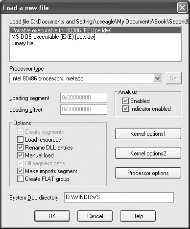
Figure 21-3 Forcing a manual load with IDA Pro
This will pull IDA Pro’s definition of the IMAGE_DOS_HEADER from its type library into your local Structures window and make it available to you. Finally, you need to return to the disassembly window, position the cursor on the first byte of the DOS header, and press ALT-Q to apply the IMAGE_DOS_HEADER template. The structure may initially appear in its collapsed form, but you can view all of the struct fields by expanding the struct with the numeric keypad + key. This results in the display shown next:

Figure 21-4 Importing the IMAGE_DOS_HEADER structure

A little research on the contents of the DOS header will tell you that the e_lfanew field holds the offset to the PE header struct. In this case, we can go to address 00400000 + 200h (00400200) and expect to find the PE header. The PE header fields can be viewed by repeating the process just described and using IMAGE_NT_HEADERS as the structure you wish to select and apply.
Quirks of Compiled C++ Code
C++ is a somewhat more complex language than C, offering member functions and polymorphism, among other things. These two features require implementation details that make compiled C++ code look rather different from compiled C code when they are used. First, all nonstatic member functions require a this pointer; and second, polymorphism is implemented through the use of vtables.
NOTE
In C++, a this pointer is available in all nonstatic member functions. This points to the object for which the member function was called and allows a single function to operate on many different objects merely by providing different values for this each time the function is called.
The means by which this pointers are passed to member functions vary from compiler to compiler. Microsoft compilers take the address of the calling object and place it in the ecx register prior to calling a member function. Microsoft refers to this calling convention as a this call. Other compilers, such as Borland and g++, push the address of the calling object as the first (leftmost) parameter to the member function, effectively making this an implicit first parameter for all nonstatic member functions. C++ programs compiled with Microsoft compilers are very recognizable as a result of their use of this call. Listing 21-8 shows a simple example.
Listing 21-8

Because Borland and g++ pass this as a regular stack parameter, their code tends to look more like traditional compiled C code and does not immediately stand out as compiled C++.
C++ Vtables
Virtual tables (vtables) are the mechanism underlying virtual functions and polymorphism in C++. For each class that contains virtual member functions, the C++ compiler generates a table of pointers called a vtable. A vtable contains an entry for each virtual function in a class, and the compiler fills each entry with a pointer to the virtual function’s implementation. Subclasses that override any virtual functions each receive their own vtable. The compiler copies the superclass’s vtable, replacing the pointers of any functions that have been overridden with pointers to their corresponding subclass implementations. The following is an example of superclass and subclass vtables:

As can be seen, the subclass overrides func3 and func4, but inherits the remaining virtual functions from its superclass. The following features of vtables make them stand out in disassembly listings:
• Vtables are usually found in the read-only data section of a binary.
• Vtables are referenced directly only from object constructors and destructors.
• By examining similarities among vtables, it is possible to understand inheritance relationships among classes in a C++ program.
• When a class contains virtual functions, all instances of that class will contain a pointer to the vtable as the first field within the object. This pointer is initialized in the class constructor.
• Calling a virtual function is a three-step process. First, the vtable pointer must be read from the object. Second, the appropriate virtual function pointer must be read from the vtable. Finally, the virtual function can be called via the retrieved pointer.
References
FLIRT reference www.hex-rays.com/idapro/flirt.htm
Hex-Rays IDA PRO Download page (FLAIR) www.hex-rays.com/idapro/idadown.htm
Extending IDA Pro
Although IDA Pro is an extremely powerful disassembler on its own, it is rarely possible for a piece of software to meet every need of its users. To provide as much flexibility as possible to its users, IDA Pro was designed with extensibility in mind. These features include a custom scripting language for automating simple tasks, and a plug-in architecture that allows for more complex, compiled extensions.
Scripting with IDC
IDA Pro’s scripting language is named IDC. IDC is a very C-like language that is interpreted rather than compiled. Like many scripting languages, IDC is dynamically typed, and can be run in something close to an interactive mode, or as complete stand-alone scripts contained in .idc files. IDA Pro does provide some documentation on IDC in the form of help files that describe the basic syntax of the language and the built-in API functions available to the IDC programmer. Like other IDA Pro documentation, what’s available for IDC follows a rather minimalist approach, consisting primarily of comments from various IDC header files. Learning the IDC API generally requires browsing the IDC documentation until you discover a function that looks like it might do what you want, and then playing around with that function until you understand how it works. The following points offer a quick rundown of the IDC language:
• IDC understands C++-style single- or multiline comments.
• No explicit data types are in IDC.
• No global variables are allowed in IDC script files.
• If you require variables in your IDC scripts, they must be declared as the first lines of your script or the first lines within any function.
• Variable declarations are introduced using the auto keyword:
auto addr, j, k, val;
auto min_ea, max_ea;
• Function declarations are introduced with the static keyword. Functions have no explicit return type. Function argument declarations do not require the auto keyword. If you want to return a value from a function, simply return it. Different control paths can return different data types:
static demoIdcFunc(val, addr) {
if (addr > 0x4000000) {
return addr + val; // return an int
}
else {
return "Bad addr"; //return a string
}
}
• IDC offers most C control structures, including if, while, for, and do. The break and continue statements are available within loops. There is no switch statement. As with C, all statements must terminate with a semicolon. C-style bracing with { and } is used.
• Most C-style operators are available in IDC. Operators that are not available include += and all other operators of the form <op>=.
• There is no array syntax available in IDC. Sparse arrays are implemented as named objects via the CreateArray, DeleteArray, SetArrayLong, SetArrayString, GetArrayElement, and GetArrayId functions.
• Strings are a native data type in IDC. String concatenation is performed using the + operator, while string comparison is performed using the == operator. There is no character data type; instead, use strings of length one.
• IDC understands the #define and #include directives. All IDC scripts executed from files must have the directive #include <idc.idc>. Interactive scripts need not include this file.
• IDC script files must contain a main function as follows:
static main() {
//idc statements
}
Executing IDC Scripts
There are two ways to execute an IDC script, both accessible via IDA Pro’s File menu. The first method is to execute a stand-alone script using File | IDC File. This will bring up a File Open dialog box in which to select the desired script to run. A stand-alone script has the following basic structure:
#include <idc.idc> //Mandatory include for standalone scripts
/*
* Other idc files may be #include'd if you have split your code
* across several files.
*
* Standalone scripts can have no global variables, but can have
* any number of functions.
*
* A standalone script must have a main function
*/
static main() {
//statements for main, beginning with any variable declarations
}
The second method for executing IDC commands is to enter just the commands you wish to execute in a dialog box provided by IDA Pro via File | IDC Command. In this case, you must not enter any function declarations or #include directives. IDA Pro wraps the statements that you enter in a main function and executes them, so only statements that are legal within the body of a function are allowed here. Figure 21-5 shows an example of the Hello World program implemented using File | IDC Command.
IDC Script Examples
While there are many IDC functions available that provide access to your IDA Pro databases, a few functions are relatively essential to know. These provide minimal access to read and write values in the database, output simple messages, and control the cursor location within the disassembly view. Byte(addr), Word(addr), and Dword(addr) read 1, 2, and 4 bytes, respectively, from the indicated address. PatchByte(addr, val), PatchWord(addr, val), and PatchDword(addr, val) patch 1, 2, and 4 bytes, respectively, at the indicated address. Note that the use of the PatchXXX functions changes only the IDA Pro database; they have no effect whatsoever on the original program binary. Message(format, ...) is similar to the C printf command, taking a format string and a variable number of arguments, and printing the result to the IDA Pro message window. If you want a carriage return, you must include it in your format string. Message provides the only debugging capability that IDC possesses, as no IDC debugger is available. Additional user interface functions are available that interact with a user through various dialog boxes. AskFile, AskYN, and AskStr can be used to display a file selection dialog box, a simple yes/no dialog box, and a simple one-line text input dialog box, respectively. Finally, ScreenEA() reads the address of the current cursor line, while Jump(addr) moves the cursor (and the display) to make addr the current address in the disassembly view.

Figure 21-5 IDC command execution
Scripts can prove useful in a wide variety of situations. Halvar Flake’s BugScam vulnerability scanner (see Chapter 20) is implemented as a set of IDC scripts. One situation in which scripts come in very handy is for decoding data or code within a binary that may have been obfuscated in some way. Scripts are useful in this case to mimic the behavior of the program in order to avoid the need to run the program. Such scripts can be used to modify the database in much the same way that the program would modify itself if it were actually running. The following script demonstrates the implementation of a decoding loop using IDC to modify a database:

IDA Pro Plug-In Modules and the IDA Pro SDK
IDC is not suitable for all situations. IDC lacks the ability to define complex data structures, perform efficient dynamic memory allocation, or access native programming APIs such as those in the C standard library or Windows API, and IDC does not provide access into the lowest levels of IDA Pro databases. Additionally, in cases where speed is required, IDC may not be the most suitable choice. For these situations, IDA Pro provides an SDK (Software Development Kit) that publishes the C++ interface specifications for the native IDA Pro API.
The IDA Pro SDK enables the creation of compiled C++ plug-ins as extensions to IDA Pro. The SDK is included with recent IDA Pro distributions or is available as a separate download from the Hex-Rays website. A new SDK is released with each new version of IDA Pro, and it is imperative that you use a compatible SDK when creating plug-ins for your version of IDA Pro. Compiled plug-ins are generally compatible only with the version of IDA Pro that corresponds to the SDK with which the plug-in was built. This can lead to problems when plug-in authors fail to provide new plug-in binaries for each new release of IDA Pro. As with other IDA Pro documentation, the SDK documentation is rather sparse. API documentation is limited to the supplied SDK header files, while documentation for compiling and installing plug-ins is limited to a few readme files. A great guide for learning to write plug-ins was published in 2005 by Steve Micallef, and covers build environment configuration as well as many useful API functions. His plug-in writing tutorial is a must read for anyone who wants to learn the nuts and bolts of IDA Pro plug-ins. See the “References” section at the end of the chapter for more details.
Basic Plug-In Concept
First, the plug-in API is published as a set of C++ header (.hpp) files in the SDK’s include directory. The contents of these files are the ultimate authority on what is or is not available to you in the IDA Pro SDK. There are two essential files that each plug-in must include: <ida.hpp> and <loader.hpp>. Ida.hpp defines the idainfo struct and the global idainfo variable inf. The inf variable is populated with information about the current database, such as processor type, program entry point, minimum and maximum virtual address values, and much more. Plug-ins that are specific to a particular processor or file format can examine the contents of the inf variable to learn whether they are compatible with the currently loaded file. Loader.hpp defines the plugin_t structure and contains the appropriate declaration to export a specific instance of a programmer-defined plugin_t. This is the single most important structure for plug-in authors, as it is mandatory to declare a single global plugin_t variable named PLUGIN. When a plug-in is loaded into IDA Pro, IDA Pro examines the exported PLUGIN variable to locate several function pointers that IDA Pro uses to initialize, execute, and terminate each plug-in. The plug-in structure is defined as follows:
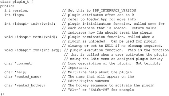
An absolutely minimal plug-in that does nothing other than print a message to IDA Pro’s message window appears next:
NOTE
wanted_hotkey is just that, the hotkey you want to use. IDA Pro makes no guarantee that your wanted_hotkey will be available, as more than one plug-in may request the same hotkey sequence. In such cases, the first plug-in that IDA Pro loads will be granted its wanted_hotkey, while subsequent plug-ins that request the same hotkey will only be able to be activated by using the Edit | Plugins menu.
#include <ida.hpp>
#include <loader.hpp>
#include <kernwin.hpp>
int idaapi my_init(void) { //idaapi marks this as stdcall
//Keep this plugin regardless of processor type
return PLUGIN_KEEP; //refer to loader.hpp for valid return values
}
void idaapi my_run(int arg) { //idaapi marks this as stdcall
//This is where we should do something interesting
static int count = 0;
//The msg function is equivalent to IDC's Message
msg("Plugin activated %d time(s)
", ++count);
}
char comment[] = "This is a simple plugin. It doesn't do much.";
char help[] =
"A simple plugin
"
"That demonstrates the basics of setting up a plugin.
"
"It doesn't do a thing other than print a message.
";
char name[] = "GrayHat plugin";
char hotkey[] = "Alt-1";
plugin_t PLUGIN = {
IDP_INTERFACE_VERSION, 0, my_init, NULL, my_run,
comment, help, name, hotkey
};
The IDA Pro SDK includes source code, along with make files and Visual Studio workspace files for several sample plug-ins. The biggest hurdle faced by prospective plug-in authors is learning the IDA Pro API. The plug-in API is far more complex than the API presented for IDC scripting. Unfortunately, plug-in API function names do not match IDC API function names; though generally if a function exists in IDC, you will be able to find a similar function in the plug-in API. Reading the Micallef’s plug-in writer’s guide along with the SDK-supplied headers and the source code to existing plug-ins is really the only way to learn how to write plug-ins.
Building IDA Pro Plug-Ins
Plug-ins are essentially shared libraries. On the Windows platform, this equates to a DLL. When building a plug-in, you must configure your build environment to build a DLL and link to the required IDA Pro libraries. The process is covered in detail in the Micallef’s plug-in writer’s guide and many examples exist to assist you. The following is a summary of configuration settings that you must make:
1. Specify build options to build a shared library.
2. Set plug-in and architecture-specific defines __IDP__, and __NT__ or __LINUX__.
3. Add the appropriate SDK library directory to your library path. The SDK contains a number of libXXX directories for use with various build environments.
4. Add the SDK include directory to your include directory path.
5. Link with the appropriate IDA Pro library (ida.lib, ida.a, or pro.a).
6. Make sure your plug-in is built with an appropriate extension (.plw for Windows, .plx for Linux).
Once you have successfully built your plug-in, installation is simply a matter of copying the compiled plug-in to IDA Pro’s plug-in directory. This is the directory within your IDA Pro program installation, not within your SDK installation. Any open databases must be closed and reopened in order for IDA Pro to scan for and load your plug-in. Each time a database is opened in IDA Pro, every plug-in in the plugins directory is loaded and its init function is executed. Only plug-ins whose init functions return PLUGIN_OK or PLUGIN_ KEEP (refer to loader.hpp) will be kept by IDA Pro. Plug-ins that return PLUGIN_SKIP will not be made available for current databases.
IDAPython Plug-In
The IDAPython plug-in by Gergely Erdelyi is an excellent example of extending the power of IDA Pro via a plug-in. The purpose of IDAPython is to make scripting both easier and more powerful at the same time. The plug-in consists of two major components: an IDA Pro plug-in written in C++ that embeds a Python interpreter into the current IDA Pro process, and a set of Python APIs that provides all of the scripting capability of IDC. By making all of the features of Python available to a script developer, IDAPython provides both an easier path to IDA Pro scripting, because users can leverage their knowledge of Python rather than learning a new language—IDC, and a much more powerful scripting interface, because all the features of Python, including data structures and APIs, become available to the script author. A similar plug-in named IdaRub was created by Spoonm to bring Ruby scripting to IDA Pro as well.
ida-x86emu Plug-In
The ida-x86emu plug-in by Chris Eagle addresses a different type of problem for the IDA Pro user, that of analyzing obfuscated code. All too often, malware samples, among other things, employ some form of obfuscation technique to make disassembly analysis more difficult. The majority of obfuscation techniques employ some form of self-modifying code that renders static disassembly listings all but useless other than to analyze the deobfuscation algorithms. Unfortunately, the deobfuscation algorithms seldom contain the malicious behavior of the code being analyzed, and as a result, the analyst is unable to make much progress until the code can be deobfuscated and disassembled yet again. Traditionally, this has required running the code under the control of a debugger until the deobfuscation has been completed, then capturing a memory dump of the process, and finally, disassembling the captured memory dump. Unfortunately, many obfuscation techniques have been developed that attempt to thwart the use of debuggers and virtual machine environments.
The ida-x86emu plug-in embeds an x86 emulator within IDA Pro and offers users the opportunity to step through disassembled code as if it were loaded into memory and running. The emulator treats the IDA Pro database as its virtual memory and provides an emulation stack, heap, and register set. If the code being emulated is self-modifying, then the emulator reflects the modifications in the loaded database. In this way, emulation becomes the tool to both deobfuscate the code and to update the IDA Pro database to reflect all self-modifications without ever running the malicious code in question. The ida-x86emu plug-in will be discussed further in Chapter 29.
IDA Pro Loaders and Processor Modules
The IDA Pro SDK can be used to create two additional types of extensions for use with IDA Pro. IDA Pro processor modules are used to provide disassembly capability for new or unsupported processor families, whereas IDA Pro loader modules are used to provide support for new or unsupported file formats. Loaders may make use of existing processor modules, or may require the creation of entirely new processor modules if the CPU type was previously unsupported. An excellent example of a loader module is one designed to parse ROM images from gaming systems. Several example loaders are supplied with the SDK in the ldr subdirectory, while several example processor modules are supplied in the module subdirectory. Loaders and processor modules tend to be required far less frequently than plug-in modules, and as a result, far less documentation and far fewer examples exist to assist in their creation. At their heart, both have architectures similar to plug-ins.
Loader modules require the declaration of a global loader_t (from loader.hpp) variable named LDSC. This structure must be set up with pointers to two functions, one to determine the acceptability of a file for a particular loader, and the other to perform the actual loading of the file into the IDA Pro database. IDA Pro’s interaction with loaders is as follows:
1. When a user chooses a file to open, IDA Pro invokes the accept_file function for every loader in the IDA Pro loaders subdirectory. The job of the accept_file function is to read enough of the input file to determine if the file conforms to the format recognized by the loader. If the accept_file function returns a nonzero value, then the name of the loader will be displayed for the user to choose from. Figure 21-3 shows an example in which the user is being offered the choice of three different ways to load the program. In this case, two different loaders (pe.ldw and dos.ldw) have claimed to recognize the file format while IDA Pro always offers the option to load a file as a raw binary file.
2. If the user elects to utilize a given loader, the loader’s load_file function is called to load the file content into the database. The job of the loader can be as complex as parsing files, creating program segments within IDA Pro, and populating those segments with the correct content from the file, or it can be as simple as passing off all of that work to an appropriate processor module.
Loaders are built in much the same manner as plug-ins, the primary difference being the file extension, which is .ldw for Windows loaders and .llx for Linux loaders. Install compiled loaders into the loaders subdirectory of your IDA Pro distribution.
IDA Pro processor modules are perhaps the most complicated modules to build. Processor modules require the declaration of a global processor_t (defined in idp.hpp) structure named LPH. This structure must be initialized to point to a number of arrays and functions that will be used to generate the disassembly listing. Required arrays define the mapping of opcode names to opcode values, the names of all registers, and a variety of other administrative data. Required functions include an instruction analyzer whose job is simply to determine the length of each instruction and to split the instruction’s bytes into opcode and operand fields. This function is typically named ana and generates no output. An emulation function, typically named emu, is responsible for tracking the flow of the code and adding additional target instructions to the disassembly queue. Output of disassembly lines is handled by the out and out_op functions, which are responsible for generating disassembly lines for display in the IDA Pro disassembly window.
There are a number of ways to generate disassembly lines via the IDA Pro API, and the best way to learn them is by reviewing the sample processor modules supplied with the IDA Pro SDK. The API provides a number of buffer manipulation primitives to build disassembly lines a piece at a time. Output generation is performed by writing disassembly line parts into a buffer and then, once the entire line has been assembled, writing the line to the IDA Pro display. Buffer operations should always begin by initializing your output buffer using the init_output_buffer function. IDA Pro offers a number of OutXXX and out_xxx functions that send output to the buffer specified in init_output_buffer. Once a line has been constructed, the output buffer should be finalized with a call to term_output_buffer before sending the line to the IDA Pro display using the printf_line function. The majority of available output functions are defined in the SDK header file ua.hpp.
Finally, one word concerning building processor modules: while the basic build process is similar to that used for plug-ins and loaders, processor modules require an additional post-processing step. The SDK provides a tool named mkidp, which is used to insert a description string into the compiled processor binary. For Windows modules, mkidp expects to insert this string in the space between the MSDOS header and the PE header. Some compilers, such as g++, in our experience do not leave enough space between the two headers for this operation to be performed successfully. The IDA Pro SDK does provide a custom DOS header stub named simply stub designed as a replacement for the default MSDOS header. Getting g++ to use this stub is not an easy task. It is recommended that Visual Studio tools be used to build processor modules for use on Windows. By default, Visual Studio leaves enough space between the MSDOS and PE headers for mkidp to run successfully. Compiled processor modules should be installed to the IDA Pro procs subdirectory.
References
Hex Blog www.hexblog.com
Hex-Rays forum www.hex-rays.com/forum
“IDA Plug-in Writing in C/C++ Tutorial” (Steve Micallef) www.binarypool.com/idapluginwriting/
IDAPython plug-in code.google.com/p/idapython/
IdaRub plug-in www.metasploit.com/users/spoonm/idarub/
ida-x86emu plug-in sourceforge.net/projects/ida-x86emu/
OpenRCE forums www.openrce.org/forums/