
Chapter 4. HBase table design
- HBase schema design concepts
- Mapping relational modeling knowledge to the HBase world
- Advanced table definition parameters
- HBase Filters to optimize read performance
In the first three chapters, you learned about interacting with HBase using the Java API and built a sample application to learn how to do so. As a part of building our TwitBase, you created tables in your HBase instance to store data in. The table definition was given to you, and you created the tables without going into the details of why you created them the way you did. In other words, we didn’t talk about how many column families to have, how many columns to have in a column family, what data should go into the column names and what should go into the cells, and so on. This chapter introduces you to HBase schema design and covers things that you should think about when designing schemas and rowkeys in HBase. HBase schemas are different from relational database schemas. They’re much simpler and provide a few things you can play with. Sometimes we refer to HBase as schema-less as well. But the simplicity gives you the ability to tweak it in order to extract optimal performance for your application’s access patterns. Some schemas may be great for writes, but when reading the same data back, these schemas may not perform as well, or vice versa.
To learn about designing HBase schemas, you’ll continue to build on the TwitBase application and introduce new features into it. Until now, TwitBase was pretty basic. You had users and twits. That’s not nearly enough functionality for an application and won’t drive user traffic unless users have the ability to be social and read other users’ twits. Users want to follow other users, so let’s build tables for that purpose.
Note
This chapter continues the approach that the book has followed so far of using a running example to introduce and explain concepts. You’ll start with a simple schema design and iteratively improve it, and we’ll introduce important concepts along the way.
4.1. How to approach schema design
TwitBase users would like to follow twits from other users, as you can imagine. To provide that ability, the first step is to maintain a list of everyone a given user follows. For instance, TheFakeMT follows both TheRealMT and HRogers. To populate all the twits that TheFakeMT should see when they log in, you begin by looking at the list {TheRealMT,HRogers} and reading the twits for each user in that list. This information needs to be persisted in an HBase table.
Let’s start thinking about the schema for that table. When we say schema, we include the following considerations:
- How many column families should the table have?
- What data goes into what column family?
- How many columns should be in each column family?
- What should the column names be? Although column names don’t have to be defined on table creation, you need to know them when you write or read data.
- What information should go into the cells?
- How many versions should be stored for each cell?
- What should the rowkey structure be, and what should it contain?
Some people may argue that a schema is only what you define up front on table creation. Others may argue that all the points in this list are part of schema design. Those are good discussions to engage in. NoSQL as a domain is relatively new, and clear definitions of terms are emerging as we speak. We feel it’s important to encompass all of these points into a broad schema design topic because the schema impacts the structure of your table and how you read or write to it. That is what you’ll do next.
4.1.1. Modeling for the questions
Let’s return to the table, which will store data about what users a particular user follows. Access to this table follows two patterns: read the entire list of users, and query for the presence of a specific user in that list, “Does TheFakeMT follow TheRealMT?” That’s a relevant question, given that TheFakeMT wants to know everything possible about the real one. In that case, you’d be interested in checking whether TheRealMT exists in the list of users TheFakeMT follows. A possible solution is to have a row for each user, with the user ID being the rowkey and each column representing a user they follow.
Remember column families? So far, you’ve used only a single column family because you haven’t needed anything more. But what about this table? All users in the list of users TheFakeMT follows have an equal chance of being checked for existence, and you can’t differentiate between them in terms of access patterns. You can’t assume that one member of this list is accessed more often than any of the others. This bit of reasoning allows you to conclude that the entire list of followed users should go into the same column family.
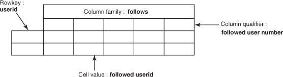
How did we come to that conclusion? All data for a given column family goes into a single store on HDFS. A store may consist of multiple HFiles, but ideally, on compaction, you achieve a single HFile. Columns in a column family are all stored together on disk, and that property can be used to isolate columns with different access patterns by putting them in different column families. This is also why HBase is called a column-family-oriented store. In the table you’re building, you don’t need to isolate certain users being followed from others. At least, that’s the way it seems right now. To store these relationships, you can create a new table called follows that looks like figure 4.1.
Figure 4.1. The follows table, which persists a list of users a particular user follows
You can create this table using the shell or the Java client, as you learned in chapter 2. Let’s look at it in a little more depth and make sure you have the optimal table design. Keep in mind that once the table is created, changing any of its column families will require that the table be taken offline.
HBase 0.92 has an experimental feature to do online schema migrations, which means you don’t need to take tables offline to change column families. We don’t recommend doing this as a regular practice. Designing your tables well up front goes a long way.
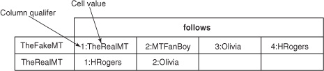
With a table design as shown in figure 4.1, a table with data looks like figure 4.2.
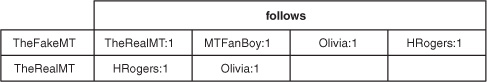
Figure 4.2. The follows table with sample data. 1:TheRealMT represents a cell in the column family follows with the column qualifier 1 and the value TheRealMT. The fake Mark Twain wants to know everything he can about the real one. He’s following not only the real Mark Twain but also his fans, his wife, and his friends. Cheeky, huh? The real Mark Twain, on the other hand, keeps it simple and only wants to get twits from his dear friend and his wife.
Now you need to validate that this table satisfies your requirements. To do so, it’s important to define the access patterns—that is, how data in your HBase tables is accessed by the application. Ideally, you should do that as early in the process as possible.
Note
Define access patterns as early in the design process as possible so they can inform your design decisions.
You aren’t too far along, so let’s do it now. To define the access patterns, a good first step is to define the questions you want to answer using this table. For instance, in TwitBase, you want this table to answer, “Whom does TheFakeMT follow?” Thinking further along those lines, you can come up with the following questions:
- Whom does TheFakeMT follow?
- Does TheFakeMT follow TheRealMT?
- Who follows TheFakeMT?
- Does TheRealMT follow TheFakeMT?
Questions 2 and 4 are basically the same; just the names have swapped places. That leaves you with the first three questions. That’s a great starting point!
“Whom does TheFakeMT follow?” can be answered by a simple get() call on the table you just designed. It gives you the entire row, and you can iterate over the list to find the users TheFakeMT follows. The code looks like this:
Get g = new Get(Bytes.toBytes("TheFakeMT"));
Result result = followsTable.get(g);
The result set returned can be used to answer questions 1 and 2. The entire list returned is the answer to question 1. You can create an array list like this:
List<String> followedUsers  = new ArrayList<String>();
List<KeyValue> list = result.list();
Iterator<KeyValue> iter = list.iterator();
while(iter.hasNext()) {
    KeyValue kv = iter.next();
    followedUsers.add(Bytes.toString(kv.getValue())) ;
}
Answering question 2 means iterating through the entire list and checking for the existence of TheRealMT. The code is similar to the previous snippet, but instead of creating an array list, you compare at each step:
String followedUser = "TheRealMT";
List<KeyValue> list = result.list();
Iterator<KeyValue> iter = list.iterator();
while(iter.hasNext()) {
     KeyValue kv = iter.next();
     if(followedUser.equals(Bytes.toString(kv.getValue())));
            return true;
}
return false;
It doesn’t get simpler than that, does it? Let’s continue building on this and ensure that your table design is the best you can accomplish and is optimal for all expected access patterns.
4.1.2. Defining requirements: more work up front always pays
You now have a table design that can answer two out of the four questions on the earlier list. You haven’t yet ascertained whether it answers the other two questions. Also, you haven’t defined your write patterns. The questions so far define the read patterns for the table.
From the perspective of TwitBase, you expect data to be written to HBase when the following things happen:
- A user follows someone
- A user unfollows someone they were following
Let’s look at the table and try to find places you can optimize based on these write patterns. One thing that jumps out is the work the client needs to do when a user follows someone new. This requires making an addition to the list of users the user is already following. When TheFakeMT follows one more user, you need to know that the user is number 5 in the list of users TheFakeMT follows. That information isn’t available to your client code without asking the HBase table. Also, there is no concept of asking HBase to add a cell to an existing row without specifying the column qualifier. To solve that problem, you have to maintain a counter somewhere. The best place to do that is the same row. In that case, the table now looks like figure 4.3.
Figure 4.3. The follows table with a counter in each row to keep track of the number of users any given user is following at the moment
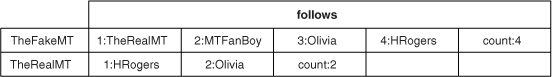
The count column gives you the ability to quickly display the number of users anyone is following. You can answer the question “How many people does TheFakeMT follow?” by getting the count column without having to iterate over the entire list. This is good progress! Also notice that you haven’t needed to change the table definition so far. That’s HBase’s schema-less data model at work.
Adding a new user to the list of followed users involves a few steps, as outlined in figure 4.4.
Figure 4.4. Steps required to add a new user to the list of followed users, based on the current table design
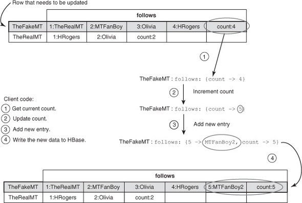
Code for adding a new user to the list of followed users looks like this:
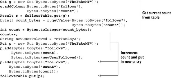
As you can see, keeping a count makes the client code complicated. Every time you have to add a user to the list of users A is following, you have to first read back the count from the HBase table, add the next user, and update the count. This process smells a lot like a transaction from the relational database systems you’ve likely worked with.
Given that HBase doesn’t have the concept of transactions, this process has a couple of issues you should be aware of. First, it isn’t thread-safe. What if the user decides to follow two different users at the same time, maybe using two different browser windows or different devices? That’s not a common occurrence, but a similar effect can happen when the user clicks the Follow button for two different users quickly, one after the other: the threads processing those requests may read back the same count, and one may overwrite the other’s work. Second, what if the client thread dies halfway through that process? You’ll have to build logic to roll back or repeat the write operation in your client code. That’s a complication you’d rather avoid.
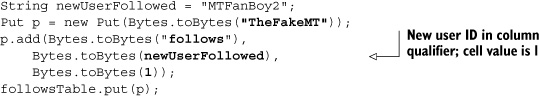
The only way you can solve this problem without making the client code complicated is to remove the counter. Again, you can use the schema-less data model to your advantage. One way to do it is to move the followed user ID into the column qualifier. Remember, HBase stores only byte[], and you can have an arbitrary number of columns within a column family. Let’s use those properties to your advantage and change the table to look like figure 4.5. You put the followed user’s username in the column qualifier instead of their position on the list of followed users. The cell value now can be anything. You need something to put there because cells can’t be empty, so you can enter the number 1. This is different from how you would design tables in relational systems.
Figure 4.5. Cells now have the followed user’s username as the column qualifier and an arbitrary string as the cell value.
Tip
Column qualifiers can be treated as data, just like values. This is different from relational systems, where column names are fixed and need to be defined up front at the time of table creation. The word column can be considered a misnomer. HBase tables are multidimensional maps.
The simplicity and flexibility of HBase’s schema allows you to make such optimizations without a lot of work but gain significant simplicity in client code or achieve greater performance.
With this new table design, you’re back to not having to keep a count, and the client code can use the followed user ID in the column qualifier. That value is always unique, so you’ll never run into the problem of overwriting existing information. The code for adding new users to the followed list becomes much simpler:
The code for reading back the list changes a little. Instead of reading back the cell values, you now read back the column qualifiers. With this change in the design, you lose the count that was available earlier. Don’t worry about it right now; we’ll teach you how to implement that functionality in the next chapter.
Tip
HBase doesn’t have the concept of cross-row transactions. Avoid designs that require transactional logic in client code, because it leads to a complex client that you have to maintain.
4.1.3. Modeling for even distribution of data and load
TwitBase may have some users who follow many people. The implication is that the HBase table you just designed will have variable-length rows. That’s not a problem per se. But it affects the read patterns. Think about the question, “Does TheFakeMT follow TheRealMT?” With this table, how can this question be answered? A simple Get request specifying TheRealMT in the rowkey and TheFakeMT as the column qualifier will do the trick. This is an extremely fast operation for HBase.
Answering the question “What’s a fast operation for HBase?” involves many considerations. Let’s first define some variables:
- n = Number of KeyValue entries (both the result of Puts and the tombstone markers left by Deletes) in the table.
- b = Number of blocks in an HFile.
- e = Number of KeyValue entries in an average HFile. You can calculate this if you know the row size.
- c = Average number of columns per row.
Note that we’re looking at this in the context of a single column family.
You begin by defining the time taken to find the relevant HFile block for a given rowkey. This work happens whether you’re doing a get() on a single row or looking for the starting key for a scan.
First, the client library has to find the correct RegionServer and region. It takes three fixed operations to get to the right region—lookup ZK, lookup -ROOT-, lookup .META.. This is an O(1)[1] operation.
1 If you who don’t have a computer science background, or if your CS is rusty, this O(n) business is called asymptotic notation. It’s a way to talk about, in this case, the worst-case runtime complexity of an algorithm. O(n) means the algorithm grows linearly with the size of n. O(1) means the algorithm runs in constant time, regardless of the size of the input. We’re using this notation to talk about the time it takes to access data stored in HBase, but it can also be used to talk about other characteristics of an algorithm, such as its memory footprint. For a primer on asymptotic notation, see http://mng.bz/4GMf.
In a given region, the row can exist in two places in the read path: in the MemStore if it hasn’t been flushed to disk yet, or in an HFile if it has been flushed. For the sake of simplicity, we’re assuming there is only one HFile and either the entire row is contained in that file or it hasn’t been flushed yet, in which case it’s in the MemStore.
Let’s use e as a reasonable proxy for the number of entries in the MemStore at any given time. If the row is in the MemStore, looking it up is O(log e) because the Mem-Store is implemented as a skip list.[2] If the row has been flushed to disk, you have to find the right HFile block. The block index is ordered, so finding the correct block is a O(log b) operation. Finding the KeyValue objects that make up the row you’re looking for is a linear scan inside the block. Once you’ve found the first KeyValue object, it’s a linear scan thereafter to find the rest of them. The scan is O(e/b), assuming that the number of cells in the row all fit into the same block. If not, the scan must access data in multiple sequential blocks, so the operation is dominated by the number of rows read, making it O(c). In other words, the scan is O(max(c, e/b)).
2 Learn more about skip lists here: http://en.wikipedia.org/wiki/Skip_list.
To sum it up, the cost of getting to a particular row is as follows:
O(1) for region lookup
+ O(log e) to locate the KeyValue in the MemStore if it’s in the MemStore or O(1) for region lookup
+ O(log b) to find the correct block in the HFile
+ O(max(c, e/b)) to find the dominating component of the scan if it has been flushed to disk
When accessing data in HBase, the dominating factor is the time taken to scan the HFile block to get to the relevant KeyValue objects. Having wide rows increases the cost of traversing the entire row during a scan. All of this assumes that you know the rowkey of the row you’re looking for.
If you don’t know the rowkey, you’re scanning an entire range of rows (possibly the entire table) to find the row you care about, and that is O(n). In this case, you no longer benefit from limiting your scan to a few HFile blocks.
We didn’t talk about the disk-seek overhead here. If the data read from the HFile is already loaded into the block cache, this sidebar’s analysis holds true. If the data needs to be read into the BlockCache from HDFS, the cost of reading the blocks from disk is much greater, and this analysis won’t hold much significance, academically speaking.
The take-away is that accessing wider rows is more expensive than accessing smaller ones, because the rowkey is the dominating component of all these indexes. Knowing the rowkey is what gives you all the benefits of how HBase indexes under the hood.
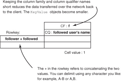
Consider the schema design shown in figure 4.6 for the follows table. Until now, you’ve been working with a table that’s designed to be a wide table. In other words, a single row contains lots of columns. The same information can be stored in the form of a tall table, which is the new schema in figure 4.6. The KeyValue objects in HFiles store the column family along with it. Keeping to short column family names makes a difference in reducing both disk and network I/O. This optimization also applies to rowkeys, column qualifiers, and even cells! Store compact representations of your data to reduce I/O load.
Figure 4.6. New schema for the follows table with the follower as well as followed user IDs in the rowkey. This translates into a single follower-followed relationship per row in the HBase table. This is a tall table instead of a wide table like the previous ones.
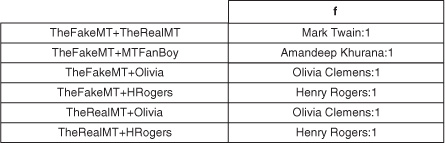
A table with some sample data is shown in figure 4.7.
Figure 4.7. The follows table designed as a tall table instead of a wide table. (And Amandeep is the fanboy we’ve been referring to so far.) Putting the user name in the column qualifier saves you from looking up the users table for the name of the user given an ID. You can simply list names or IDs while looking at relationships just from this table. The downside is that you need to update the name in all the cells if the user updates their name in their profile. This is classic de-normalization.
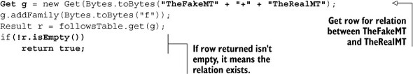
This new design for the table makes answering the second question, “Does TheFakeMT follow TheRealMT?” faster than it is with some of the previous designs. You can get() on a row with rowkey TheFakeMT+TheRealMT and get your answer. There’s only one cell in the column family, so you don’t need multiple KeyValues as in the previous design. In HBase, accessing a single narrow row resident in the BlockCache is the fastest possible read operation.
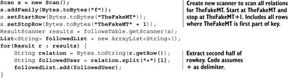
Answering the first question, “Whom does TheFakeMT follow?” becomes an index lookup to the first block with a prefix of TheFakeMT followed by a scan on subsequent rows with rowkeys starting with TheFakeMT. From an I/O standpoint, you’re reading the same amount of data from the RegionServer when scanning those rows as compared to doing a Get on a single wide row and iterating over all the cells. Remember the HFile design? The physical storage for both the table designs mentioned is essentially the same. The physical indexing is what changed, as we’ll discuss a little later.
The code for getting the list of followed users now looks like this:
The code for checking whether a relationship exists between two users looks like this:
To add to the list of followed users, you do a simple put() as follows:
Put p = new Put(Bytes.toBytes("TheFakeMT" + "+" + "TheRealMT");
p.add(Bytes.toBytes("f"), Bytes.toBytes(newFollowedUser), Bytes.toBytes(1));
followsTable.put(p);
Tip
The get() API call is internally implemented as a scan() operation scanning over a single row.
Tall tables aren’t always the answer to table design. To gain the performance benefits of a tall table, you trade off atomicity for certain operations. In the earlier design, you could update the followed list for any user with a single Put operation on a row. Put operations at a row level are atomic. In the second design, you give up the ability to do that. In this case, it’s okay because your application doesn’t require that. But other use cases may need that atomicity, in which case wide tables make more sense.
Note
You give up atomicity in order to gain performance benefits that come with a tall table.
A good question to ask here is, why put the user ID in the column qualifier? It isn’t necessary to do that. Think about TwitBase and what users may be doing that translates into reading this table. Either they’re asking for a list of all the people they follow or they’re looking at someone’s profile to see if they’re following that user. Either way, the user ID isn’t enough. The user’s real name is more important. That information is stored in the users table at this point. In order to populate the real name for the end user, you have to fetch it from the user table for each row in the follows table that you’ll return to the user. Unlike in a relational database system, where you do a join and can accomplish all this in a single SQL query, here you have to explicitly make your client read from two different tables to populate all the information you need. To simplify, you could de-normalize[3] and put the username in the column qualifier, or, for that matter, in the cell in this table. But it’s not hunky-dory if you do this. This approach makes maintaining consistency across the users table and the follows table a little challenging. That’s a trade-off you may or may not choose to make. The intention of doing it here is to expose you to the idea of de-normalizing in HBase and the reasoning behind it. If you expect your users to change their names frequently, de-normalizing may not be a good idea. We’re assuming that their names are relatively static content and de-normalizing won’t cost you much.
3 If this is the first time you’ve come across the term de-normalization, it will be useful to read up on it before you proceed. Essentially, you’re increasing the replication of data, paying more in storage and update costs, to reduce the number of accesses required to answer a question and speed overall access times. A good place to start is http://en.wikipedia.org/wiki/Denormalization.
Tip
De-normalize all you can without adding complexity to your client code. As of today, HBase doesn’t provide the features that make normalization easy to do.
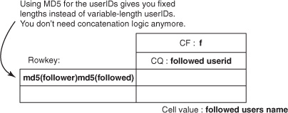
You can use another optimization to simplify things. In the twits table, you used MD5 as the rowkey. This gave you a fixed-length rowkey. Using hashed keys has other benefits, too. Instead of having userid1+userid2 as the rowkey in the follows table, you can instead have MD5(userid1)MD5(userid2) and do away with the + delimiter. This gives you two benefits. First, your rowkeys are all of consistent length, giving you more predictability in terms of read and write performance. That’s probably not a huge win if you put a limit on the user ID length. The other benefit is that you don’t need the delimiter any more; it becomes simpler to calculate start and stop rows for the scans.
Using hashed keys also buys you a more uniform distribution of data across regions. In the example you’ve been working with so far, distribution isn’t a problem. It becomes a problem when your access patterns are skewed inherently and you’re at risk of hot-spotting on a few regions rather than spreading the load across the entire cluster.
Hot-spotting in the context of HBase means there is a heavy concentration of load on a small subset of regions. This is undesirable because the load isn’t distributed across the entire cluster. Overall performance becomes bottlenecked by the few hosts that are serving those regions and thereby doing a majority of the work.
For instance, if you’re inserting time-series data, and the timestamp is at the beginning of the rowkey, you’re always appending to the bottom of the table because the timestamp for any write is always greater than any timestamp that has already been written. So, you’ll hot-spot on the last region of the table.
If you MD5 the timestamp and use that as the rowkey, you achieve an even distribution across all regions, but you lose the ordering in the data. In other words, you can no longer scan a small time range. You need either to read specific timestamps or scan the entire table. You haven’t lost getting access to records, though, because your clients can MD5 the timestamp before making the request.
Hash functions can be defined as functions that map a large value of variable length to a smaller value of fixed length. There are various types of hashing algorithms, and MD5 is one of them. MD5 produces a 128-bit (16-byte) hash value for any data you hash. It’s a popular hash function that you’re likely to come across in various places; you probably already have.
Hashing is an important technique in HBase specifically and in information-retrieval implementations in general. Covering these algorithms in detail is beyond the scope of this text. If you want to learn more about the guts of hashing and the MD5 algorithm, we recommend finding an online resource.
4 Message-Digest Algorithm: http://en.wikipedia.org/wiki/MD5.
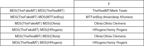
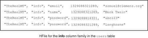
The follows table looks like figure 4.8 if you use MD5s in the rowkeys. By storing MD5s of the user IDs in the rowkey, you can’t get back the user IDs when you read back. When you want the list of users Mark Twain follows, you get the MD5s of the user IDs instead of the user IDs. But the name of the user is stored in the column qualifier because you want to store that information as well. To make the user ID accessible, you can put it into the column qualifier and the name into the cell value.
Figure 4.8. Using MD5s as part of rowkeys to achieve fixed lengths and better distribution
The table looks like figure 4.9 with data in it.
Figure 4.9. Using MD5 in the rowkey lets you get rid of the + delimiter that you needed so far. The rowkeys now consist of fixed-length portions, with each user ID being 16 bytes.
4.1.4. Targeted data access
At this point, you may wonder what kind of indexing is taking place in HBase. We’ve talked about it in the last two chapters, but it becomes important when thinking about your table designs. The tall table versus wide table discussion is fundamentally a discussion of what needs to be indexed and what doesn’t. Putting more information into the rowkey gives you the ability to answer some questions in constant time. Remember the read path and block index from chapter 2? That’s what’s at play here, enabling you to get to the right row quickly.
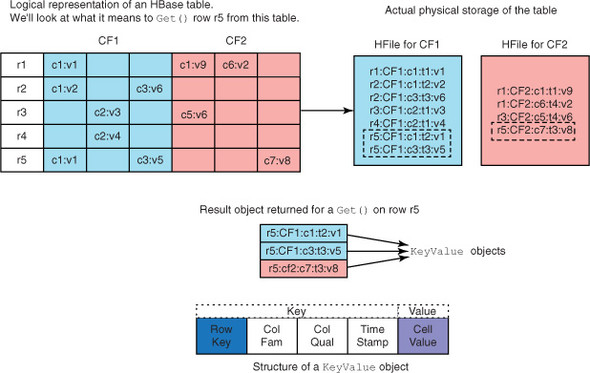
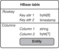
Only the keys (the Key part of the KeyValue object, consisting of the rowkey, column qualifier, and timestamp) are indexed in HBase tables. Think of it as the primary key in a relational database system, but you can’t change the column that forms the primary key, and the key is a compound of three data elements (rowkey, column qualifier, and timestamp). The only way to access a particular row is through the rowkey. Indexing the qualifier and timestamp lets you skip to the right column without scanning all the previous columns in that row. The KeyValue object that you get back is basically a row from the HFile, as shown in figure 4.10.
Figure 4.10. Logical to physical translation of an HBase table. The KeyValue object represents a single entry in the HFile. The figure shows the result of executing get(r5) on the table to retrieve row r5.
There are two ways to retrieve data from a table: Get and Scan. If you want a single row, you use a Get call, in which case you have to provide the rowkey. If you want to execute a Scan, you can choose to provide the start and stop rowkeys if you know them, and limit the number of rows the scanner object will scan.
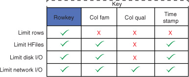
When you execute a Get, you can skip to the exact block that contains the row you’re looking for. From there, it scans the block to find the relevant KeyValue objects that form the row. In the Get object, you can also specify the column family and the column qualifiers if you want. By specifying the column family, you can limit the client to accessing only the HFiles for the specified column families. Specifying the column qualifier doesn’t play a role in limiting the HFiles that are read off the disk, but it does limit what’s sent back over the wire. If multiple HFiles exist for a column family on a given region, all of them are accessed to find the components of the row you specify in the Get call. This access is regardless of how many HFiles contain data relevant to the request. Being as specific as possible in your Get is useful, though, so you don’t transfer unnecessary data across the wire to the client. The only cost is potential disk I/O on the RegionServer. If you specify timestamps in your Get object, you can avoid reading HFiles that are older than that timestamp. Figure 4.11 illustrates this in a simple table.
Figure 4.11. Depending on what part of the key you specify, you can limit the amount of data you read off the disk or transfer over the network. Specifying the rowkey lets you read just the exact row you need. But the server returns the entire row to the client. Specifying the column family lets you further specify what part of the row to read, thereby allowing for reading only a subset of the HFiles if the row spans multiple families. Further specifying the column qualifier and timestamp lets you save on the number of columns returned to the client, thereby saving on network I/O.
You can use this information to inform your table design. Putting data into the cell value occupies the same amount of storage space as putting it into the column qualifier or the rowkey. But you can possibly achieve better performance by moving it up from the cell to the rowkey. The downside to putting more in the rowkey is a bigger block index, given that the keys are the only bits that go into the index.
You’ve learned quite a few things so far, and we’ll continue to build on them in the rest of the chapter. Let’s do a quick recap before we proceed:
- HBase tables are flexible, and you can store anything in the form of byte[].
- Store everything with similar access patterns in the same column family.
- Indexing is done on the Key portion of the KeyValue objects, consisting of the rowkey, qualifier, and timestamp in that order. Use it to your advantage.
- Tall tables can potentially allow you to move toward O(1) operations, but you trade atomicity.
- De-normalizing is the way to go when designing HBase schemas.
- Think how you can accomplish your access patterns in single API calls rather than multiple API calls. HBase doesn’t have cross-row transactions, and you want to avoid building that logic in your client code.
- Hashing allows for fixed-length keys and better distribution but takes away ordering.
- Column qualifiers can be used to store data, just like cells.
- The length of column qualifiers impacts the storage footprint because you can put data in them. It also affects the disk and network I/O cost when the data is accessed. Be concise.
- The length of the column family name impacts the size of data sent over the wire to the client (in KeyValue objects). Be concise.
Having worked through an example table design process and learned a bunch of concepts, let’s solidify some of the core ideas and look at how you can use them while designing HBase tables.
4.2. De-normalization is the word in HBase land
One of the key concepts when designing HBase tables is de-normalization. We’ll explore it in detail in this section. So far, you’ve looked at maintaining a list of the users an individual user follows. When a TwitBase user logs in to their account and wants to see twits from the people they follow, your application fetches the list of followed users and their twits, returning that information. This process can take time as the number of users in the system grows. Moreover, if a user is being followed by lots of users, their twits are accessed every time a follower logs in. The region hosting the popular user’s twits is constantly answering requests because you’ve created a read hot spot. The way to solve that is to maintain a twit stream for every user in the system and add twits to it the moment one of the users they follow writes a twit.
Think about it. The process for displaying a user’s twit stream changes. Earlier, you read the list of users they follow and then combined the latest twits for each of them to form the stream. With this new idea, you’ll have a persisted list of twits that make up a user’s stream. You’re basically de-normalizing your tables.
Normalization is a technique in the relational database world where every type of repeating information is put into a table of its own. This has two benefits: you don’t have to worry about the complexity of updating all copies of the given data when an update or delete happens; and you reduce the storage footprint by having a single copy instead of multiple copies. The data is recombined at query time using JOIN clauses in SQL statements.
De-normalization is the opposite concept. Data is repeated and stored at multiple locations. This makes querying the data much easier and faster because you no longer need expensive JOIN clauses.
From a performance standpoint, normalization optimizes for writes, and de-normalization optimizes for reads.
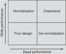
Normalization optimizes the table for writes; you pay the cost of combining data at read time. De-normalization optimizes for reads, but you pay the cost of writing multiple copies at write time.
In this case, you can de-normalize by having another table for twit streams. By doing this, you’ll take away the read-scalability issue and solve it by having multiple copies of the data (in this case, a popular user’s twits) available for all readers (the users following the popular user).
As of now, you have the users table, the twits table, and the follows table. When a user logs in, you get their twit stream by using the following process:
- Get a list of people the user follows.
- Get the twits for each of those followed users.
- Combine the twits and order them by timestamp, latest first.
You can use a couple of options to de-normalize. You can add another column family to the users table and maintain a stream there for each user. Or you can have another table for twit streams. Putting the twit stream in the users table isn’t ideal because the rowkey design of that table is such that it isn’t optimal for what you’re trying to do. Keep reading; you’ll see this reasoning soon.
The access pattern for the twit stream table consists of two parts:
- Reading a list of twits to show to a given user when the user logs in, and displaying it in reverse order of creation timestamp (latest first)
- Adding to the list of twits for a user when any of the users they follow writes a twit
Another thing to think about is the retention policy for the twit stream. You may want to maintain a stream of the twits from only the last 72 hours, for instance. We talk about Time To Live (TTL) later, as a part of advanced column family configurations.
Using the concepts that we’ve covered so far, you can see that putting the user ID and the reverse timestamp in the rowkey makes sense. You can easily scan a set of rows in the table to retrieve the twits that form a user’s twit stream. You also need the user ID of the person who created each twit. This information can go into the column qualifier. The table looks like figure 4.12.
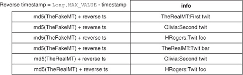
Figure 4.12. A table to store twit streams for every user. Reverse timestamps let you sort the twits with the latest twit first. That allows for efficient scanning and retrieval of the n latest twits. Retrieving the latest twits in a user’s stream involves scanning the table.
When someone creates a twit, all their followers should get that twit in their respective streams. This can be accomplished using coprocessors, which we talk about in the next chapter. Here, we can talk about what the process is. When a user creates a twit, a list of all their followers is fetched from the relationships table, and the twit is added to each of the followers’ streams. To accomplish this, you need to first be able to find the list of users following any given user, which is the inverse of what you’ve solved so far in your relationships table. In other words, you want to answer the question, “Who follows me?” effectively.
With the current table design, this question can be answered by scanning the entire table and looking for rows where the second half of the rowkey is the user you’re interested in. Again, this process is inefficient. In a relational database system, this can be solved by adding an index on the second column and making a slight change to the SQL query. Also keep in mind that the amount of data you would work with is much smaller. What you’re trying to accomplish here is the ability to perform these kinds of operations with large volumes of data.
4.3. Heterogeneous data in the same table
HBase schemas are flexible, and you’ll use that flexibility now to avoid doing scans every time you want a list of followers for a given user. The intent is to expose you to the various ideas involved in designing HBase tables. The relationships table as you have it now has the rowkey as follows:
md5(user) + md5(followed user)
You can add the relationship information to this key and make it look like this:
md5(user) + relationship type + md5(user)
That lets you store both kinds of relationships in the same table: following as well as followed by. Answering the questions you’ve been working with so far now involves checking for the relationship information from the key. When you’re accessing all the followers for a particular user or all the users a particular user is following, you’ll do scans over a set of rows. When you’re looking for a list of users for the first case, you want to avoid having to read information for the other case. In other words, when you’re looking for a list of followers for a user, you don’t want a list of users that the user follows in the dataset returned to your client application. You can accomplish this by specifying the start and end keys for the scan.
Let’s look at another possible key structure: putting the relationship information in the first part of the key. The new key looks like this:
relationship type + md5(user) + md5(user)
Think about how the data is distributed across the RegionServers now. Everything for a particular type of relationship is collocated. If you’re querying for a list of followers more often than the followed list, the load isn’t well distributed across the various regions. That is the downside of this key design and the challenge in storing heterogeneous data in the same table.
Tip
Isolate different access patterns as much as possible.
The way to improve the load distribution in this case is to have separate tables for the two types of relationships you want to store. You can create a table called followedBy with the same design as the follows table. By doing that, you avoid putting the relationship type information in the key. This allows for better load distribution across the cluster.
One of the challenges we haven’t addressed yet is keeping the two relationship entries consistent. When Mark Twain decides to follow his fanboy, two entries need to be made in the tables: one in the follows table and the other in the followedBy table. Given that HBase doesn’t allow inter-table or inter-row transactions, the client application writing these entries has to ensure that both rows are written. Failures happen all the time, and it will make the client application complicated if you try to implement transactional logic there. In an ideal world, the underlying database system should handle this for you; but design decisions are different at scale, and this isn’t a solved problem in the field of distributed systems at this point.
4.4. Rowkey design strategies
By now, you may have seen a pattern in the design process you went through to come up with the two tables to store relationship information. The thing you’ve been tweaking is the rowkey.
Tip
In designing HBase tables, the rowkey is the single most important thing. You should model keys based on the expected access pattern.
Your rowkeys determine the performance you get while interacting with HBase tables. Two factors govern this behavior: the fact that regions serve a range of rows based on the rowkeys and are responsible for every row that falls in that range, and the fact that HFiles store the rows sorted on disk. These factors are interrelated. HFiles are formed when regions flush the rows they’re holding in memory; these rows are already in sorted order and get flushed that way as well. This sorted nature of HBase tables and their underlying storage format allows you to reason about performance based on how you design your keys and what you put in your column qualifiers. To refresh your memory about HFiles, look at figure 4.13; it’s the HFile you read about in chapter 2.
Figure 4.13. The conceptual structure of an HFile
Unlike relational databases, where you can index on multiple columns, HBase indexes only on the key; the only way to access data is by using the rowkey. If you don’t know the rowkey for the data you want to access, you’ll end up scanning a chunk of rows, if not the entire table. There are various techniques to design rowkeys that are optimized for different access patterns, as we’ll explore next.
4.5. I/O considerations
The sorted nature of HBase tables can turn out to be a great thing for your application—or not. For instance, when we looked at the twit stream table in the previous section, its sorted nature gave you the ability to quickly scan a small set of rows to find the latest twits that should show up in a user’s stream. But the same sorted nature can hurt you when you’re trying to write a bunch of time-series data into an HBase table (remember hot-spotting?). If you choose your rowkey to be the timestamp, you’ll always be writing to a single region, whichever is responsible for the range in which the timestamp falls. In fact, you’ll always be writing to the end of a table, because timestamps are monotonically increasing in nature. This not only limits your throughput to what a single region can handle but also puts you at risk of overloading a single machine where other machines in the cluster are sitting idle. The trick is to design your keys such that they’re optimized for the access pattern you care about.
4.5.1. Optimized for writes
When you’re writing lots of data into HBase tables, you want to optimize by distributing the load across RegionServers. This isn’t all that hard to do, but you may have to make trade-offs in optimizing your read patterns: for instance, the time-series data example. If your data is such that you use the timestamp as the rowkey, you’ll hot-spot on a single region during write time.
In many use cases, you don’t need to access the data based on a single timestamp. You’ll probably want to run a job that computes aggregates over a time range, and if that’s not latency sensitive, you can afford to do a parallel scan across multiple regions to do that for you. The question is, how do you distribute that data across multiple regions? There are a few options to consider, and the answer depends on what kind of information you want your rowkeys to contain.
Hashing
If you’re willing to lose the timestamp information from your rowkey (which may be okay in cases where you need to scan the entire table every time you want to do something, or you know the exact key every time you want to read data), making your rowkey a hash of the original data is a possible solution:
hash("TheRealMT") -> random byte[]
You need to know "TheRealMT" every time you want to access the row that is keyed by the hashed value of this function.
With time-series data, that generally isn’t the case. You most likely don’t know the specific timestamp when you access data; you probably have a time range in mind. But there are cases like the twits table or the relationship tables you created earlier, where you know the user ID and can calculate the hash to find the correct row. To achieve a good distribution across all regions, you can hash using MD5, SHA-1, or any other hash function of your choice that gives you random distribution.
Hashing algorithms have a non-zero probability of collision. Some algorithms have more than others. When working with large datasets, be careful to use a hashing algorithm that has lower probability of collision. For instance, SHA-1 is better than MD5 in that regard and may be a better option in some cases even though it’s slightly slower in performance.
The way you use your hash function is also important. The relationship tables you built earlier in this chapter use MD5 hashes of the user IDs, but you can easily regenerate those when you’re looking for a particular user’s information. But note that you’re concatenating the MD5 hashes of two user IDs (MD5(user1) + MD5(user2)) rather than concatenating the user IDs and then hashing the result (MD5(user1 + user2)). The reason is that when you want to scan all the relationships for a given user, you pass start and stop rowkeys to your scanner object. Doing that when the key is a hash of the combination of the two user IDs isn’t possible because you lose the information for the given user ID from that rowkey.
Salting
Salting is another trick you can have in your tool belt when thinking about rowkeys. Let’s consider the same time-series example discussed earlier. Suppose you know the time range at read time and don’t want to do full table scans. Hashing the timestamp and making the hash value the rowkey requires full table scans, which is highly inefficient, especially if you have the ability to limit the scan. Making the hash value the rowkey isn’t your solution here. You can instead prefix the timestamp with a random number.
For example, you can generate a random salt number by taking the hash code of the timestamp and taking its modulus with some multiple of the number of Region-Servers:
int salt = new Integer(new Long(timestamp).hashCode()).shortValue() % <number
     of region servers>
This involves taking the salt number and putting it in front of the timestamp to generate your timestamp:
byte[] rowkey = Bytes.add(Bytes.toBytes(salt)
+ Bytes.toBytes("|") + Bytes.toBytes(timestamp));
Now your rowkeys are something like the following:
0|timestamp1
0|timestamp5
0|timestamp6
1|timestamp2
1|timestamp9
2|timestamp4
2|timestamp8
These, as you can imagine, distribute across regions based on the first part of the key, which is the random salt number.
0|timestamp1, 0|timestamp5, and 0|timestamp6 go to one region unless the region splits, in which case it’s distributed to two regions. 1|timestamp2 and 1|timestamp9 go to a different region, and 2|timestamp4 and 2|timestamp8 go to the third. Data for consecutive timestamps is distributed across multiple regions.
But not everything is hunky-dory. Reads now involve distributing the scans to all the regions and finding the relevant rows. Because they’re no longer stored together, a short scan won’t cut it. It’s about trade-offs and choosing the ones you need to make in order to have a successful application.
4.5.2. Optimized for reads
Optimizing rowkeys for reads was your focus while designing the twit stream table. The idea was to store the last few twits for a user’s stream together so they could be fetched quickly without having to do disk seeks, which are expensive. It’s not just the disk seeks but also the fact that if the data is stored together, you have to read a smaller number of HFile blocks into memory to read the dataset you’re looking for; data is stored together, and every HFile block you read gives you more information per read than if the data were distributed all over the place. In the twit stream table, you used reverse timestamps (Long.MAX_VALUE - timestamp) and appended it to the user ID to form the rowkey. Now you need to scan from the user ID for the next n rows to find the n latest twits the user must see. The structure of the rowkey is important here. Putting the user ID first allows you to configure your scan so you can easily define your start rowkey. That’s the topic we discuss next.
4.5.3. Cardinality and rowkey structure
The structure of the rowkey is of utmost importance. Effective rowkey design isn’t just about what goes into the rowkey, but also about where elements are positioned in the rowkey. You’ve already seen two cases of how the structure impacted read performance in the examples you’ve been working on.
First was the relationship table design, where you put the relationship type between the two user IDs. It didn’t work well because the reads became inefficient. You had to read (at least from the disk) all the information for both types of relationships for any given user even though you only needed information for one kind of relationship. Moving the relationship type information to the front of the key solved that problem and allowed you to read only the data you needed.
Second was the twit stream table, where you put the reverse timestamp as the second part of the key and the user ID as the first. That allowed you to scan based on user IDs and limit the number of rows to fetch. Changing the order there resulted in losing the information about the user ID, and you had to scan a time range for the twits, but that range contained twits for all users with something in that time range.
For the sake of creating a simple example, consider the reverse timestamps to be in the range 1..10. There are three users in the system: TheRealMT, TheFakeMT, and Olivia. If the rowkey contains the user ID as the first part, the rowkeys look like the following (in the order that HBase tables store them):
Olivia1
Olivia2
Olivia5
Olivia7
Olivia9
TheFakeMT2
TheFakeMT3
TheFakeMT4
TheFakeMT5
TheFakeMT6
TheRealMT1
TheRealMT2
TheRealMT5
TheRealMT8
But if you flip the order of the key and put the reverse timestamp as the first part, the rowkey ordering changes:
1Olivia
1TheRealMT
2Olivia
2TheFakeMT
2TheRealMT
3TheFakeMT
4TheFakeMT
5Olivia
5TheFakeMT
5TheRealMT
6TheFakeMT
7Olivia
8TheRealMT
9Olivia
Getting the last n twits for any user now involves scanning the entire time range because you can no longer specify the user ID as the start key for the scanner.
Now look back at the time-series data example, where you added a salt as a prefix to the timestamp to form the rowkey. That was done to distribute the load across multiple regions at write time. You had only a few ranges to scan at read time when you were looking for data from a particular time range. This is a classic example of using the placement of the information to achieve distribution across the regions.
Tip
Placement of information in your rowkey is as important as the information you choose to put into it.
We have explored several concepts about HBase table design in this chapter thus far. You may be at a place where you understand everything and are ready to go build your application. Or you may be trying to look at what you just learned through the lens of what you already know in the form of relational database table modeling. The next section is to help you with that.
4.6. From relational to non-relational
You’ve likely used relational database systems while building applications and been involved in the schema design. If that’s not the case and you don’t have a relational database background, skip this section. Before we go further into this conversation, we need to emphasize the following point: There is no simple way to map your relational database knowledge to HBase. It’s a different paradigm of thinking.
If you find yourself in a position to migrate from a relational database schema to HBase, our first recommendation is don’t do it (unless you absolutely have to). As we have said on several occasions, relational databases and HBase are different systems and have different design properties that affect application design. A naïve migration from relational to HBase is tricky. At best, you’ll create a complex set of HBase tables to represent what was a much simpler relational schema. At worst, you’ll miss important but subtle differences steeped in the relational system’s ACID guarantees. Once an application has been built to take advantage of the guarantees provided by a relational database, you’re better off starting from scratch and rethinking your tables and how they can serve the same functionality to the application.
Mapping from relational to non-relational isn’t a topic that has received much attention so far. There is a notable master’s thesis[5] that explores this subject. But we can draw some analogies and try to make the learning process a little easier. In this section, we’ll map relational database modeling concepts to what you’ve learned so far about modeling HBase tables. Things don’t necessarily map 1:1, and these concepts are evolving and being defined as the adoption of NoSQL systems increases.
5 Ian Thomas Varley, “No Relation: The Mixed Blessing of Non-Relational Databases,” Master’s thesis, http://mng.bz/7avI.
4.6.1. Some basic concepts
Relational database modeling consists of three primary concepts:
- Entities—These map to tables.
- Attributes—These map to columns.
- Relationships—These map to foreign-key relationships.
The mapping of these concepts to HBase is somewhat convoluted.
Entities
A table is just a table. That’s probably the most obvious mapping from the relational database world to HBase land. In both relational databases and HBase, the default container for an entity is a table, and each row in the table should represent one instance of that entity. A user table has one user in each row. This isn’t an iron-clad rule, but it’s a good place to start. HBase forces you to bend the rules of normalization, so a lot of things that are full tables in a relational database end up being something else in HBase. Soon you’ll see what we mean.
Attributes
To map attributes to HBase, you must distinguish between (at least) two types:
- Identifying attribute—This is the attribute that uniquely identifies exactly one instance of an entity (that is, one row). In relational tables, this attribute forms the table’s primary key. In HBase, this becomes part of the rowkey, which, as you saw earlier in the chapter, is the most important thing to get right while designing HBase tables.
Often an entity is identified by multiple attributes. This maps to the concept of compound keys in relational database systems: for instance, when you define relationships. In the HBase world, the identifying attributes
make up the rowkey, as you saw in the tall version of the follows table. The rowkey was formed by concatenating the user IDs of the users that formed the relationship. HBase doesn’t have
the concept of compound keys, so both identifying attributes had to be put into the rowkey.
Using values of fixed length makes life much easier. Variable lengths mean you need delimiters and escaping logic in your
client code to figure out the composite attributes that form the key. Fixed length also makes it easier to reason about start
and stop keys. A way to achieve fixed length is to hash the individual attributes as you did in the follows table.
Note
It’s common practice to take multiple attributes and make them a part of the rowkey, which is a byte[]. Remember, HBase doesn’t care about types.
- Non-identifying attribute—Non-identifying attributes are easier to map. They basically map to column qualifiers in HBase. For the users table that you built earlier in the book, non-identifying attributes were things like the password and the email address. No uniqueness guarantees are required on these attributes.
As explained earlier in this chapter, each key/value (for example, the fact that user TheRealMT has a state of Missouri) carries its entire set of coordinates around with it: rowkey, column family name, column qualifier, and timestamp. If you have a relational database table with wide rows (dozens or hundreds of columns), you probably don’t want to store each of those columns as a column in HBase (particularly if most operations deal with mutating the entire row at a time). Instead, you can serialize all the values in the row into a single binary blob that you store as the value in a single cell. This takes a lot less disk space, but it has downsides: the values in the row are now opaque, and you can’t use the structure that HBase tables have to offer. When the storage footprint (and hence the disk and network I/O) are important and the access patterns always involve reading entire rows, this approach makes sense.
Relationships
Logical relational models use two main varieties of relationships: one-to-many and many-to-many. Relational databases model the former directly as foreign keys (whether explicitly enforced by the database as constraints, or implicitly referenced by your application as join columns in queries) and the latter as junction tables (additional tables where each row represents one instance of a relationship between the two main tables). There is no direct mapping of these in HBase, and often it comes down to de-normalizing the data.
The first thing to note is that HBase, not having any built-in joins or constraints, has little use for explicit relationships. You can just as easily place data that is one-to-many in nature into HBase tables: one table for users and another for their twits. But this is only a relationship in that some parts of the row in the former table happen to correspond to parts of rowkeys in the latter table. HBase knows nothing of this relationship, so it’s up to your application to do things with it (if anything). As mentioned earlier, if the job is to return all the twits for all the users you follow, you can’t rely on a join or subquery to do this, as you can in SQL:
SELECT * FROM twit WHERE user_id IN
(SELECT user_id from followees WHERE follower = me)
ORDER BY date DESC limit 10;
Instead, you need to write code outside of HBase that iterates over each user and then does a separate HBase lookup for that user to find their recent twits (or else, as explained previously, de-normalize copies of the twits for each follower).
As you can see, outside of implicit relationships enforced by some external application, there’s no way to physically connect disparate data records in HBase. At least not yet!
4.6.2. Nested entities
One thing that’s significantly different about HBase is that the columns (also known as column qualifiers) aren’t predefined at design time. They can be anything. And in an earlier example, an early version of the follows table had one row for the user and one column for each follower (first with an integer counter for the column qualifier, then with the followed username as the qualifier). Note that far from being a flexible schema row, this represents the ability to nest another entity inside the row of a parent or primary entity (figure 4.14).
Figure 4.14. Nesting entities in an HBase table
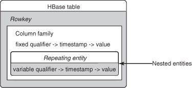
Nested entities are another tool in your relational-to-non-relational tool belt: if your tables exist in a parent-child, master-detail, or other strict one-to-many relationship, it’s possible to model it in HBase as a single row. The rowkey will correspond to the parent entity. The nested values will contain the children, where each child entity gets one column qualifier into which their identifying attributes are stored, with the remainder of the non-identifying attributes stashed into the value (concatenated together, for example). The real HBase row defines the parent record (and can have some normal columns, too); records of the child entity are stored as individual columns (figure 4.15).
Figure 4.15. HBase tables can contain regular columns along with nested entities.
As an added bonus, in this pattern you do get transactional protection around the parent and child records, because in HBase, the row is the boundary of transactional protection. So you can do check and put operations and generally be sure that all your modifications are wrapped up and commit or fail together.
You can put in nested entities by using HBase’s flexibility because of the way columns are designed. HBase doesn’t necessarily have special abilities to store nested entities.
There are some limitations to this, of course. First, this technique only works to one level deep: your nested entities can’t themselves have nested entities. You can still have multiple different nested child entities in a single parent, and the column qualifier is their identifying attributes.
Second, it’s not as efficient to access an individual value stored as a nested column qualifier inside a row, as compared to accessing a row in another table, as you learned earlier in the chapter.
Still, there are compelling cases where this kind of schema design is appropriate. If the only way you get at the child entities is via the parent entity, and you’d like to have transactional protection around all children of a parent, this can be the right way to go.
Things get a little trickier with many-to-many relationships. HBase doesn’t help you with optimized joins or any such thing; but you don’t get off easy by nesting an entity, because each relationship has two parents. This often translates to de-normalization, as it did in the case of the follows table earlier in the chapter. You de-normalized the follower relationship, which is a self-referential many-to-many relationship on users.
These are the basic foundations of mapping your relational modeling knowledge to concepts in the HBase world.
4.6.3. Some things don’t map
So far, you’ve mapped a bunch of concepts from the relational world to HBase. We haven’t talked about column families yet. It turns out there’s no direct analogue in the relational world! Column families exist in HBase as a way for a single row to contain disjoint sets of columns in a way that’s physically efficient but can be processed atomically. Unless you use a column-oriented database like Vertica, or special analytical features of the commercial relational databases, this isn’t something relational databases do.
Column Families
One way of thinking about column families is that they model yet another kind of relationship that we didn’t talk about previously: the one-to-one relationship, where you have two tables with the same primary key, and each table has either 0 or 1 row with each primary key value. An example is user personal information (email address, birthday, and so on) versus user system preferences (background color, font size, and so on). It’s common to model these as two separate physical tables in a relational database, with the thought that because your SQL statements nearly always hit one or the other, but not both, they may perform more optimally if you separate the tables. (This depends heavily on which database you’re using and a million other factors, but it does happen.)
In HBase, this is a perfect case for using two column families in a single table. And, likewise, the nested entity relationships mentioned earlier can easily be partitioned into separate column families, on the assumption that you’d likely not access both together.
Generally speaking, using multiple column families in HBase is an advanced feature that you should only jump into if you’re sure you understand the trade-offs.
(Lack of) Indexes
Another common question when migrating from a relational database to HBase is: what about indexes? In relational databases, the ability to easily declare indexes that are automatically maintained by the database engine is one of the most magical and helpful capabilities the software provides, and it’s nowhere to be found in HBase. For now, the answer to this question is: tough luck.
You can make some approximation of this feature by de-normalizing data and writing it into multiple tables, but make no mistake: when you move to HBase, you’re explicitly giving up the warm, comfortable world where a simple CREATE INDEX statement solves big performance problems and gets your boss off your back. In HBase, you have to work through all those questions up front and design your access patterns into your schema.
Versioning
There’s one final interesting angle on the relationship between relational databases and non-relational ones: the time dimension. If, in your relational schema, there are places where you explicitly store timestamps, these can in many cases be subsumed into the timestamp that’s stored in HBase cells. Beware that this is only a long, so if you need more than UNIX-era timestamps held in a 64-bit long, that’s all you get in HBase timestamps (thus they’re probably not right for storing the granules of time in atomic simulations).
Even better, if your application currently goes out of its way to store historical versions of values in a table (in a pattern often referred to as the history table pattern, where you use the same primary key from the main table coupled with a timestamp, in order to preserve all copies of rows over time): rejoice! You can dump that dumb idea and replace it with a single HBase entity, and set the number of versions to keep appropriately in the column family metadata. This is an area that’s significantly easier in HBase; the original architects of relational models didn’t want to consider time to be a special dimension outside of the relational model, but let’s face it: it is.
We hope you now have a good sense of what all those years of studying relational database design bought you in the move to HBase. If you understand the basics of logical modeling and know what schema dimensions are available in HBase, you’ve got a fighting chance of preserving the intent of your designs.
4.7. Advanced column family configurations
HBase has a few advanced features that you can use when designing your tables. These aren’t necessarily linked to the schema or the rowkey design but define aspects of the behavior of the tables. In this section, we’ll cover these various configuration parameters and how you can use them to your advantage.
4.7.1. Configurable block size
The HFile block size can be configured at a column family level. This block is different from HDFS blocks that we talked about earlier. The default value is 65,536 bytes, or 64 KB. The block index stores the starting key of each HFile block. The block size configuration affects the size of the block index size. The smaller the block size, the larger the index, thereby yielding a bigger memory footprint. It gives you better random lookup performance because smaller blocks need to be loaded into memory. If you want good sequential scan performance, it makes sense to load larger chunks of the HFile into the memory at once, which means setting the block size to a larger value. The index size shrinks and you trade random read performance.
You can set the block size during table instantiation like this:
hbase(main):002:0> create 'mytable',
{NAME => 'colfam1', BLOCKSIZE => '65536'}
4.7.2. Block cache
Often, workloads don’t benefit from putting data into a read cache—for instance, if a certain table or column family in a table is only accessed for sequential scans or isn’t accessed a lot and you don’t care if Gets or Scans take a little longer. In such cases, you can choose to turn off caching for those column families. If you’re doing lots of sequential scans, you’re churning your cache a lot and possibly polluting it for data that you can benefit by having in the cache. By disabling the cache, you not only save that from happening but also make more cache available for other tables and other column families in the same table.
By default, the block cache is enabled. You can disable it at the time of table creation or by altering the table:
hbase(main):002:0> create 'mytable',
{NAME => 'colfam1', BLOCKCACHE => 'false'}
4.7.3. Aggressive caching
You can choose some column families to have a higher priority in the block cache (LRU cache). This comes in handy if you expect more random reads on one column family compared to another. This configuration is also done at table-instantiation time:
hbase(main):002:0> create 'mytable',
{NAME => 'colfam1', IN_MEMORY => 'true'}
The default value for the IN_MEMORY parameter is false. Setting it to true isn’t done a lot in practice because no added guarantees are provided except the fact that HBase will try to keep this column family in the block cache more aggressively than the other column families.
4.7.4. Bloom filters
The block index provides an effective way to find blocks of the HFiles that should be read in order to access a particular row. But its effectiveness is limited. The default size of an HFile block is 64 KB, and this size isn’t tweaked much.
If you have small rows, indexing just the starting rowkey for an entire block doesn’t give you indexing at a fine granularity. For example, if your rows have a storage footprint of 100 bytes, a 64 KB block contains (64 * 1024)/100 = 655.53 = ~700 rows, for which you have only the start row as the indexed bit. The row you’re looking for may fall in the range of a particular block but doesn’t necessarily have to exist in that block. There can be cases where the row doesn’t exist in the table or resides in a different HFile or even the MemStore. In that case, reading the block from disk brings with it I/O overhead and also pollutes the block cache. This impacts performance, especially when you’re dealing with a large dataset and lots of concurrent clients trying to read it.
Bloom filters allow you to apply a negative test to the data stored in each block. When a request is made for a specific row, the bloom filter is checked to see whether that row is not in the block. The bloom filter says conclusively that the row isn’t present, or says that it doesn’t know. That’s why we say it’s a negative test. Bloom filters can also be applied to the cells within a row. The same negative test is made when accessing a specific column qualifier.
Bloom filters don’t come for free. Storing this additional index layer takes more space. Bloom filters grow with the size of the data they index, so a row-level bloom filter takes up less space than a qualifier-level bloom filter. When space isn’t a concern, they allow you to squeeze that much additional performance out of the system.
You enable bloom filters on the column family, like this:
hbase(main):007:0> create 'mytable',
{NAME => 'colfam1', BLOOMFILTER => 'ROWCOL'}
The default value for the BLOOMFILTER parameter is NONE. A row-level bloom filter is enabled with ROW, and a qualifier-level bloom filter is enabled with ROWCOL. The row-level bloom filter checks for the non-existence of the particular rowkey in the block, and the qualifier-level bloom filter checks for the non-existence of the row and column qualifier combination. The overhead of the ROWCOL bloom filter is higher than that of the ROW bloom filter.
4.7.5. TTL
Often, applications have the flexibility or requirement to delete old data from their databases. Traditionally, a lot of flexibility was built in because scaling databases beyond a certain point was hard. In TwitBase, for instance, you wouldn’t want to delete any twits generated by users in the course of their use of the application. This is all human-generated data and may turn out to be useful at a future date when you want to do some advanced analytics. But it isn’t a requirement to keep all those twits accessible in real time. Twits older than a certain period can be archived into flat files.
HBase lets you configure a TTL in seconds at the column family level. Data older than the specified TTL value is deleted as part of the next major compaction. If you have multiple versions on the same cell, the versions that are older than the configured TTL are deleted. You can disable the TTL, or make it forever by setting the value to INT.MAX_VALUE (2147483647), which is the default value. You can set the TTL while creating the table like this:
hbase(main):002:0> create 'mytable', {NAME => 'colfam1', TTL => '18000'}
This command sets the TTL on the column family colfam1 as 18,000 seconds = 5 hours. Data in colfam1 that is older than 5 hours is deleted during the next major compaction.
4.7.6. Compression
HFiles can be compressed and stored on HDFS. This helps by saving on disk I/O and instead paying with a higher CPU utilization for compression and decompression while writing/reading data. Compression is defined as part of the table definition, which is given at the time of table creation or at the time of a schema change. It’s recommended that you enable compression on your tables unless you know for a fact that you won’t benefit from it. This can be true in cases where either the data can’t be compressed much or your servers are CPU bound for some reason.
Various compression codecs are available to be used with HBase, including LZO, Snappy, and GZIP. LZO[6] and Snappy[7] are among the more popular ones. Snappy was released by Google in 2011, and support was added into the Hadoop and HBase projects soon after its release. Prior to this, LZO was the codec of choice. The LZO native libraries that need to be used with Hadoop are GPLv2-licensed and aren’t part of any of the HBase or Hadoop distributions; they must be installed separately. Snappy, on the other hand, is BSD-licensed, which makes it easier to bundle with the Hadoop and HBase distributions. LZO and Snappy have comparable compression ratios and encoding/decoding speeds.
6 Lempel-Ziv-Oberhumer compression algorithm: www.oberhumer.com/opensource/lzo/.
7 Snappy compression library, by Google: http://code.google.com/p/snappy/.
You can enable compression on a column family when creating tables like this:
hbase(main):002:0> create 'mytable',
{NAME => 'colfam1', COMPRESSION => 'SNAPPY'}
Note that data is compressed only on disk. It’s kept uncompressed in memory (Mem-Store or block cache) or while transferring over the network.
It shouldn’t happen often, but if you want to change the compression codec being used for a particular column family, doing so is straightforward. You need to alter the table definition and put in the new compression scheme. The HFiles formed as a part of compactions thereafter will all be compressed using the new codec. There is no need to create new tables and copy data over. But you have to ensure that the old codec libraries aren’t deleted from the cluster until all the old HFiles are compacted after this change.
4.7.7. Cell versioning
HBase by default maintains three versions of each cell. This property is configurable. If you care about only one version, it’s recommended that you configure your tables to maintain only one. This way, it doesn’t hold multiple versions for cells you may update. Versions are also configurable at a column family level and can be specified at the time of table instantiation:
hbase(main):002:0> create 'mytable', {NAME => 'colfam1', VERSIONS => 1}
You can specify multiple properties for column families in the same create statement, like this:
hbase(main):002:0> create 'mytable',
                  {NAME => 'colfam1', VERSIONS => 1, TTL => '18000'}
You can also specify the minimum versions that should be stored for a column family like this:
hbase(main):002:0> create 'mytable', {NAME => 'colfam1', VERSIONS => 5,
                                      MIN_VERSIONS => '1'}
This comes in handy in conjunction with setting the TTLs on the family. When all versions currently stored are older than the TTL, at least the MIN_VERSION number of last versions is kept around. This ensures that you don’t get empty results if you query and the data is older than the TTL.
4.8. Filtering data
You’ve learned so far that HBase has a flexible schema and a simple disk layout, which allows applications to work closer to the disk and network and optimize at that level. Designing effective schemas is one aspect of it, and by now you have a bunch of concepts that you can apply to do that. You can design your keys such that data you access together is placed close on the disk so you can save on disk seeks while reading or writing. Often you have certain criteria, based on which you’re reading data that you can use to further optimize access. Filters are a powerful feature that can come in handy in such cases.
We haven’t come across many real-life use cases that use filters much; generally the access pattern can be optimized with tweaks to the table designs. But sometimes you’ve tweaked your table design as much as you can, and optimized it for as many different access patterns as possible. When you still need to reduce the data returned to clients, that’s when you reach for a filter. Filters are sometimes called push-down predicates, allowing you to push data-filtering criteria down to the server (see figure 4.16). That logic is applied during reads and affects the data that is returned to the client. This saves network I/O by limiting the data transferred over the network. But data is still read off the disk into the RegionServers, and filters are applied at the RegionServers. The network I/O savings can be significant because you’re probably storing a large amount of data in HBase tables, and reading it all into the client application to filter out useful bits is expensive.
Figure 4.16. Filtering data can be done at the client side by reading data into the client application from the RegionServers and applying the filter logic there; or it can be done at the server side by pushing the filtering logic down to the RegionServers, thereby reducing the amount of data transferred over the network to the clients. Filters can essentially save on network I/O costs, and sometimes even on disk I/O.
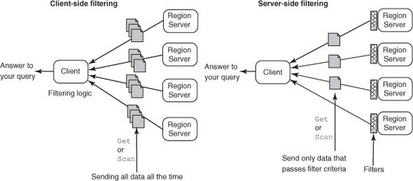
HBase provides an API you can use to implement custom filters. A bunch of filters come bundled as well. Filtering can be done based on the rowkeys, which happens the earliest in the read process. Thereafter, filtering can happen based on the KeyValues read off the HFiles. A filter has to implement the Filter interface that’s part of the HBase JAR or extend one of the abstract classes that implement it. We recommend extending the FilterBase abstract class so you can avoid having to write boilerplate code. Extending other classes such as CompareFilter is also an option and works equally well. The interface has the following methods that are called at various points while reading a row (see figure 4.17 for the order). They’re always executed in the sequence described next:
- This method is the first one to be called and performs filtering based on the rowkey:
boolean filterRowKey(byte[] buffer, int offset, int length) Based on the logic in there, it returns true if the row is to be filtered out (not included in the result set returned) or false if it’s to be sent to the client. - If the row isn’t filtered in the previous step, this method is invoked next for every KeyValue object that’s part of the current row:
ReturnCode filterKeyValue(KeyValue v) This method returns a ReturnCode, which is an enum defined as a part of the Filter interface. The ReturnCode returned determines what happens to that particular KeyValue object. - This method comes after the KeyValues are filtered based on step 2:
void filterRow(List<KeyValue> kvs) This method is passed the list of KeyValue objects that made it after filtering. Given that this method has access to that list, you can perform any transformations or operations you want to on the elements in the list at this point. - At this point, the framework provides another chance to filter out the row if you choose to do so:
boolean filterRow() Returning true filters out the row under consideration. - You can build logic in your filter to stop a scan early. This is the method into which you put that logic:
boolean filterAllRemaining() This is handy in cases where you’re scanning a bunch of rows, looking for something specific in the rowkey, column qualifier, or cell value, and you don’t care about the remaining rows once you’ve found it. This is the last method to be called in the filtering process.
Figure 4.17. The steps during the filtering process. This happens for each row in the range that is being scanned by the scanner object.
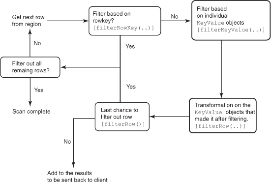
Another useful method is reset(). It resets the filter and is called by the server after it has been applied to the entire row.
Note
This API is powerful, but we aren’t aware of it being used much in applications. In many cases, the requirement for using filters changes if the schema design is changed.
4.8.1. Implementing a filter
You’ve been building TwitBase, and as the application has matured and gained users, you realize that the password strength policy you have in place for new users doesn’t ensure passwords that are secure enough. This brings about a new policy, albeit a simple one: TwitBase now requires all users to have a password that’s at least four characters long. This will apply to new and old users alike. To enforce this policy on old users, you need to go through the entire list of users and check for password length. In cases where it’s less than four characters, the password needs to be expired and a notification sent across informing the user of the new policy and the action they need to take: resetting their password to something that’s at least six characters long.
You’ll implement this using a custom filter that checks the length of the value in the cell. This filter can be applied to a scan (or to a MapReduce job), which outputs only the users to whom the password change notification has to be sent. The output is the user’s name, user ID, and email address. You’ll implement this using a scan, but you can easily convert it to a MapReduce job.
The filter you need to build is concerned only about the value in the password cell and not about anything else. The filtering logic goes in the filterKeyValue(..) method, where the password column is checked. If the password is shorter than the minimum required length, the row is included in the results; otherwise it’s excluded. The inclusion/exclusion of the row is done by the filterRow() method.
Listing 4.1. Implementing a custom filter to check password length
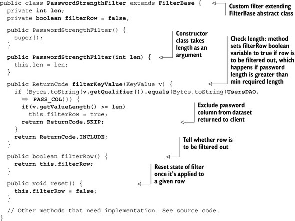
To install custom filters, you have to compile them into a JAR and put them in the HBase classpath so they get picked up by the RegionServers at startup time. In a running system, you have to restart your cluster. The custom filter you just wrote is available in the GitHub project in the package HBaseIA.TwitBase.filters by the name PasswordStrengthFilter. To compile the JAR, in the top-level directory of the project, do the following:
mvn install
cp target/twitbase-1.0.0.jar /my/folder/
Now, edit your hbase-env.sh file in $HBASE_HOME/conf and put the path of the created JAR into the classpath variable.
export HBASE_CLASSPATH=/my/folder/twitbase-1.0.0.jar
Restart the HBase process.
This filter can be used in a scan as follows:
HTable t = new HTable(UsersDAO.TABLE_NAME);
Scan scan = new Scan();
scan.addColumn(UsersDAO.INFO_FAM, UsersDAO.PASS_COL);
scan.addColumn(UsersDAO.INFO_FAM, UsersDAO.NAME_COL);
scan.addColumn(UsersDAO.INFO_FAM, UsersDAO.EMAIL_COL);
Filter f = new PasswordStrengthFilter(4);
scan.setFilter(f);
This usage filters out all rows where the password length is greater than or equal to four characters and returns rows with the names and emails of the users whose passwords don’t match the minimum length requirement. The password field isn’t returned because its KeyValue object is excluded in the filter.
This code is available in the PasswordStrengthFilterExample class in the same project. To run the code, you can do the following:
java -cp target/twitbase-1.0.0.jar
 HBaseIA.TwitBase.filters.PasswordStrengthFilterExample
4.8.2. Prebundled filters
HBase ships with numerous filters bundled along, so you may not need to implement your own. To see a comprehensive list, we recommend that you look at the javadocs. We’ll cover some of the more commonly used ones here.
RowFilter
RowFilter is a comparison filter that comes bundled and allows you to filter data based on rowkeys. You can do exact matches, substring matches, or regular-expression matches and filter out data that doesn’t match. To instantiate RowFilter, you have to provide a comparison operator and the value you want to compare. The constructor is as follows:
public RowFilter(CompareOp rowCompareOp,
                   WritableByteArrayComparable rowComparator)
The comparison operators are defined in CompareOp, which is an enum defined in the CompareFilter abstract class and can have the following values:
- LESS—Checks whether the value is less than the one provided in the comparator
- LESS_OR_EQUAL—Checks whether the value is less than or equal to the comparator
- EQUAL—Checks whether the value is equal to the comparator
- NOT_EQUAL—Checks whether the value is not equal to the comparator
- GREATER_OR_EQUAL—Checks whether the value is greater than or equal to the comparator
- GREATER—Checks whether the value is greater than the comparator
- NO_OP—Returns false by default, thereby filtering out everything
The comparator has to extend the WritableByteArrayComparable abstract class. The prebundled comparator types available are as follows:
- BinaryComparator—Compares using the Bytes.compareTo() method
- BinaryPrefixComparator—Does a prefix-based bytewise comparison using Bytes.compareTo(), starting from the left
- NullComparator—Checks whether the given value is null
- BitComparator—Does a bitwise comparison
- RegexStringComparator—Compares the passed value with the regular expression provided at the time of instantiating the comparator
- SubstringComparator—Does a contains() check in the passed value for the substring provided as a part of the comparator
Here are some examples of how to use RowFilter:
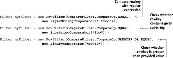
PrefixFilter
This is a special case of RowFilter. Use it to filter based on a prefix value of the rowkey. It’s similar to providing an end key to the Scan(byte[] startRow, byte[] stopRow) constructor, except you don’t need to calculate stopRow yourself. This is useful because calculating stopRow correctly can sometimes be tricky when taking byte[] overflow into account. PrefixFilter isn’t smart enough to skip ahead to the first matching startRow, so be sure to provide it. It’s smart enough to end the scan once it finds the first rowkey that doesn’t match the prefix.
Use PrefixFilter like this:
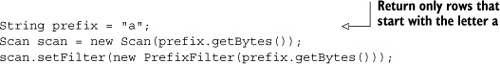
QualifierFilter
QualifierFilter is a comparison filter like RowFilter, except it matches the column qualifier name rather than the rowkey. It uses the same comparison operators and comparator types as RowFilter. There is a filter to match the column family name as well, but it isn’t as interesting as QualifierFilter. Besides, you can limit the scan or get operation to a particular column family.
You use QualifierFilter like this:
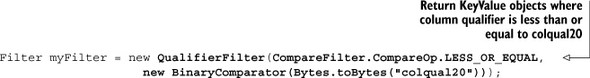
Like a scan, you can apply any filter to a Get object, but not all of them make sense. For instance, filtering a Get based on the rowkey isn’t useful. But you can filter out columns being returned in a Get using QualifierFilter.
ValueFilter
ValueFilter provides the same functionality as RowFilter or QualifierFilter, but over cell values. Using this filter allows you to filter out all cells that don’t match the provided criteria:
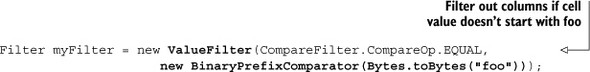
TimestampFilter
This filter allows much finer-grained control over the versions that are returned to the client. You provide a list of timestamps that should be returned, and only cells with a matching timestamp are returned.
If you want a time range when you’re scanning or retrieving individual rows, you can use the setTimeRange(..) method on the Get or Scan object to enforce that. The filter, on the other hand, lets you specify a list of timestamps that should be matched:
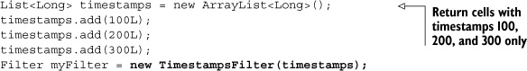
FilterList
Often it’s useful to combine multiple filters. Suppose you’re looking to get back all rows that match a certain regular expression but are interested in cells that contain a particular word. In that case, you can combine filters into a FilterList object and pass it to the scanner. The FilterList class also implements the Filter interface and can be used to create filtering logic that combines multiple individual filters.
You can configure the filter list in two modes: MUST_PASS_ALL or MUST_PASS_ONE. As the names suggest, the modes include results in the final list if they pass all filters or if they pass only one filter, respectively:

The filters are applied in the order that the List object gives them back. So, you can choose to have finer control based on the type of list object you use or by inserting the filters in the list in a particular order.
The Filtering API is powerful and has features that allow you to optimize disk seeks. This not only saves network I/O but also saves on disk I/O. To see the usage of this feature, look at the ColumnPrefixFilter, which is one of the bundled filters that ships with HBase.
4.9. Summary
This chapter covered a lot of material. We’re glad you made it to the end and hope you learned a few things along the way. In many ways, HBase provides a new approach to data management. That’s true both in the capabilities of the system as well as in the best practices around using that system. With any luck, this chapter has opened your eyes to the considerations that must be addressed when designing HBase tables as well as the feature trade-offs you make when you decide to work with or without a relational system. We’ll do our best to recap.
It’s about the questions, not the relationships. When designing for HBase, it’s about efficiently looking up the answer to a question, not purity of the entity model. You must make this trade-off because distributed transactions bottleneck concurrency and distributed joins are network-bound. Never in section 4.1.1 did we ask, “How can the data be modeled for efficient storage?” Instead we focused on answering queries efficiently.
Design is never finished. You have to put something on paper and run it through some scenarios to see where it breaks down. Allow your schema to evolve. De-normalization is both a powerful friend and a frightful foe. There’s always a trade-off between the response time of reads and the complexity of writes. Maximize the number of questions you can answer with a given design, and then tweak it to support two new access patterns. Your users will thank you.
Scale is a first-class entity. When building on HBase or any other distributed system, distribution of workload is always a concern. These tools are designed to handle a huge volume of traffic spread across the cluster. A build-up of traffic, or hot spot, on any single member of the cluster is catastrophic. Because of that, you must always keep the even distribution of that load in the back of your mind. HBase gives you the ability to design that load into your schema. Use it wisely.
Every dimension is an opportunity. HBase has multiple indexes over multiple dimensions of the physical data model. Every one of them is exposed to you directly. This is as much a challenge as it is empowering. If you can’t figure out how to answer that last question, step back and see if there’s an index you haven’t taken advantage of yet. Seeing these opportunities is a big part of why it’s important to understand how HBase works under the hood.
Remember, designing your rowkey is the single most important decision you can make. Take full advantage of the flexibility of the logical data model. Scans are your friend, but use them wisely and for the right access patterns. And remember, when all else fails, you can always fall back on a custom filter.
Now that you’re equipped with the tricks of the trade when it comes to designing HBase tables, the next two chapters are about extending HBase to add interesting functionality that you may want for your application. Chapters 7 and 8 are dedicated to exploring how HBase can be used to solve real-world problems; you’ll learn practical use of some of the techniques covered in this chapter.