Chapter 7. HBase by example: OpenTSDB

 

 

In this chapter, we want to give you a sense of what it’s like to build applications against HBase. What better way is there to learn a technology than to see first-hand how it can be used to solve a familiar problem? Rather than continuing on with our contrived example, we’ll look at an existing application: OpenTSDB. Our goal is to show you what an application backed by HBase looks like, so we won’t skimp on the gritty details.

How is building an application against HBase different than building for other databases? What are the primary concerns when designing an HBase schema? How can you take advantage of these designs when implementing your application code? These are the questions we’ll answer throughout this chapter. By the time we’re through, you’ll have a good idea of what it takes to build an application on HBase. Perhaps more important, you’ll have insight into how to think like an HBase application designer.

To start, we’ll give you some context. You’ll gain an understanding of what OpenTSDB is and what challenge it solves. Then we’ll peel back the layers, exploring the design of both the application and the database schema. After that, you’ll see how OpenTSDB uses HBase. You’ll see the application logic necessary for storing and retrieving data from HBase and how this data is used to build informative charts for the user.

7.1. An overview of OpenTSDB

What is OpenTSDB? Here’s a description taken directly from the project homepage (www.opentsdb.net):

OpenTSDB is a distributed, scalable Time Series Database (TSDB) written on top of HBase. OpenTSDB was written to address a common need: store, index, and serve metrics collected from computer systems (network gear, operating systems, applications) at a large scale, and make this data easily accessible and graphable.

OpenTSDB is a great project for a practical book because it solves the pervasive problem of infrastructure monitoring. If you’ve deployed a production system, you know the importance of infrastructure monitoring. Don’t worry if you haven’t; we’ll fill you in. It’s also interesting because the data OpenTSDB stores is time series. Efficient storage and querying of time-series data is something for which the standard relational model isn’t well suited. Relational database vendors often look to nonstandard solutions for this problem, such as storing the time-series data as an opaque blob and providing proprietary query extensions for its introspection.

 

 

OpenTSDB was built at StumbleUpon, a company highly experienced with HBase. It’s a great example of how to build an application with HBase as its backing store. OpenTSDB is open source, so you have complete access to the code. The entire project is less than 15,000 lines of Java so it can easily be digested in its entirety. OpenTSDB is ultimately a tool for online data visualization. While studying the schema, keep this in mind. Every data point it stores in HBase must be made available to the user, on demand, in a chart like the one shown in figure 7.1.

Figure 7.1. OpenTSDB graph output.^[1] OpenTSDB is a tool for visualizing data. Ultimately it’s about providing insight into the data it stores in graphs like this one.

¹Graph reproduced directly from the OpenTSDB website.

That’s OpenTSDB in a nutshell. Next we’ll look more closely at the challenge OpenTSDB is designed to solve and the kinds of data it needs to store. After that, we’ll consider why HBase is a good choice for an application like OpenTSDB. Let’s look now at infrastructure monitoring so you can understand how the problem domain motivates the schema.

7.1.1. Challenge: infrastructure monitoring

Infrastructure monitoring is the term we use for keeping tabs on deployed systems. The vast majority of software projects are deployed as online systems and services communicating over a network. Odds are, you’ve deployed a system like this, which means odds are you’ve found it your professional responsibility to maintain that system. How did you know if the system was up or down? Did you keep track of how many requests it served every hour or what times of the day it sustained the most traffic? If you’ve been paged in the night because a service went down, you’ve worked with infrastructure-monitoring tools.

Infrastructure monitoring is much more than notification and alerting. The series of events that triggered your midnight alarm represent only a small amount of the total data those tools collect. Relevant data points include service requests per second, concurrent active user sessions, database reads and writes, average response latency, process memory consumption, and so on. Each of these is a time-series measurement associated with a specific metric and individually provides only a small snapshot of visibility into overall system operation. Take these measurements together along a common time window, and you begin to have an actionable view of the running system.

Generating a graph like the one in figure 7.1 requires that data be accessible by metric as well as time interval. OpenTSDB must be able to collect a variety of metrics from a huge number of systems and yet support online queries against any of those metrics. You’ll see in the next section how this requirement becomes a key consideration in the OpenTSDB schema design.

We’ve mentioned time series more than a few times because it also plays a critical role in the design of OpenTSDB’s schema. Let’s become more familiar with this kind of data.

7.1.2. Data: time series

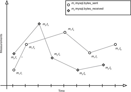
Think of time-series data as a collection of data points or tuples. Each point has a timestamp and a measurement. This set of points ordered by time is the time-series. The measurements are usually collected at a regular interval. For instance, you might use OpenTSDB to collect bytes sent by the MySQL process every 15 seconds. In this case, you would have a series of points like those in figure 7.2. It’s common for these data points to also carry metadata about the measurement, such as the fully qualified hostname generating the series.

Figure 7.2. A time series is a sequence of time-ordered points. Here, two time series on the same scale are rendered on the same graph. They don’t share a common interval. The timestamp is commonly used as an X-axis value when representing a time series visually.

Time-series data is commonly found in economics, finance, natural sciences, and signal processing. By attaching a timestamp to a measurement, we can understand differences between measurement values as time progresses and also understand patterns over time. For instance, the current temperature at a particular location can be measured every hour. It’s natural to assume previous points can inform a future point. You could guess the next hour’s temperature based on the last five hours’ measurements.

Time-series data can be challenging from a data-management perspective. All data points in a system may share the same fields, for instance: date/time, location, and measurement. But two data points with different values for any one of these fields might be completely unrelated. If one point is the temperature in New York and another in San Francisco, they’re likely not related even with a similar timestamp. How do we know how to store and order the data in a way that is relevant and efficient? Shouldn’t we store all measurements for New York close together?

Another notable issue with time series is in recording this data. Trees are an efficient data structure for random access, but special care must be taken when building them in sorted order. A time series is naturally ordered by time and is often persisted according to that order. This can result in the storage structures being built in the worst possible way, as illustrated by (b) in figure 7.3.

Figure 7.3. Balanced and unbalanced trees. Persisting data into structures that arrange themselves based on data values can result in worst-case data distribution.

Just like a tree, this ordering can also cause havoc on a distributed system. HBase is a distributed B-Tree, after all. When data is partitioned across nodes according to the timestamp, new data bottlenecks at a single node, causing a hot spot. As the number of clients writing data increases, that single node is easily overwhelmed.

That’s time-series data in a nutshell. Now let’s see what HBase can bring to the table for the OpenTSDB application.

7.1.3. Storage: HBase

HBase makes an excellent choice for applications such as OpenTSDB because it provides scalable data storage with support for low-latency queries. It’s a general-purpose data store with a flexible data model, which allows OpenTSDB to craft an efficient and relatively customized schema for storing its data. In this case, that schema is customized for time-series measurements and their associated tags. HBase provides strong consistency, so reports generated by OpenTSDB can be used for real-time reporting. The view of collected data HBase provides is always as current as possible. The horizontal scalability of HBase is critical because of the data volume required of OpenTSDB.

Certainly other databases could be considered. You could back a system like OpenTSDB with MySQL, but what would that deployment look like after a month of collecting hundreds of millions of data points per day? After six months? After 18 months of your application infrastructure running in production, how will you have grown and extended that original MySQL machine to cope with the volume of monitoring data produced by your datacenter? Suppose you’ve grown this deployment with the data produced, and you’re able to maintain your clustered deployment. Can you serve the ad-hoc queries required by your operational team for diagnosing a system outage?

All this is possible with a traditional relational database deployment. There’s an impressive list of stories describing massive, successful deployments of these technologies. The question comes down to cost and complexity. Scaling a relational system to cope with this volume of data requires a partitioning strategy. Such an approach often places the burden of partitioning in the application code. Your application can’t request a bit of data from the database. Instead, it’s forced to resolve which database hosts the data in question based on its current knowledge of all available hosts and all ranges of data. Plus, in partitioning the data, you lose a primary advantage of relational systems: the powerful query language. Partitioned data is spread across multiple systems unaware of each other, which means queries are reduced to simple value lookups. Any further query complexity is again pressed to client code.

HBase hides the details of partitioning from the client applications. Partitions are allocated and managed by the cluster so your application code remains blissfully unaware. That means less complexity for you to manage in your code. Although HBase doesn’t support a rich query language like SQL, you can design your HBase schema such that most of your online query complexity resides on the cluster. HBase coprocessors give you the freedom to embed arbitrary online code on the nodes hosting the data, as well. Plus, you have the power of MapReduce for offline queries, giving you a rich variety of tools for constructing your reports. For now, we’ll focus on one specific example.

At this point you should have a feel for the goals of OpenTSDB and the technical challenges those goals present. Let’s dig into the details of how to design an application to meet these challenges.

7.2. Designing an HBase application

Although OpenTSDB could have been built on a relational database, it’s an HBase application. It’s built by individuals who think about scalable data systems in the same way HBase does. This is different than the way we typically think about relational data systems. These differences can be seen in both the schema design and application architecture of OpenTSDB.

This section begins with a study of the OpenTSDB schema. For many of you, this will be your first glimpse of a nontrivial HBase schema. We hope this working example will provide useful insight into taking advantage of the HBase data model. After that, you’ll see how to use the key features of HBase as a model for your own applications.

7.2.1. Schema design

OpenTSDB depends on HBase for two distinct functions. The tsdb table provides storage and query support over time-series data. The tsdb-uid table maintains an index of globally unique values for use as metric tags. We’ll first look at the script used to generate these two tables and dive deeper into the usage and design of each one. First, let’s look at the script.

Listing 7.1. Scripting the HBase shell to create the tables used by OpenTSDB

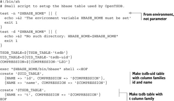
The first thing to notice is how similar the script is to any script containing Data Definition Language (DDL) code for a relational database. The term DDL is often used to distinguish code that provides schema definition and modification from code performing data updates. A relational database uses SQL for schema modifications; HBase depends on the API. As you’ve seen, the most convenient way to access the API for this purpose is through the HBase shell.

Declaring the Schema

The tsdb-uid table contains two column families: id and name. The tsdb table also specifies a column family, named t. Notice that the lengths of the column-family names are all pretty short. This is because of an implementation detail of the HFile storage format of the current version of HBase—shorter names mean less data to store per KeyValue instance. Notice, too, the lack of a higher-level abstraction. Unlike most popular relational databases, there is no concept of table groups. All table names in HBase exist in a common namespace managed by the HBase master.

Now that you’ve seen how these two tables are created in HBase, let’s explore how they’re used.

The TSDB-UID Table

Although this table is ancillary to the tsdb table, we explore it first because understanding why it exists will provide insight into the overall design. The OpenTSDB schema design is optimized for the management of time-series measurements and their associated tags. By tags, we mean anything used to further identify a measurement recorded in the system. In OpenTSDB, this includes the observed metric, the metadata name, and the metadata value. It uses a single class, UniqueId, to manage all of these different tags, hence uid in the table name. Each metric in figure 7.2, mysql.bytes_sent and mysql.bytes_received, receives its own unique ID (UID) in this table.

The tsdb-uid table is for UID management. UIDs are of a fixed 3-byte width and used in a foreign-key relationship from the tsdb table; more on that later. Registering a new UID results in two rows in this table, one mapping tag name-to-UID, the other is UID-to-name. For instance, registering the mysql.bytes_sent metric generates a new UID used as the rowkey in the UID-to-name row. The name column family for that row stores the tag name. The column qualifier is used as a kind of namespace for UIDs, distinguishing this UID as a metric (as opposed to a metadata tag name or value). The name-to-UID row uses the name as the row key and stores the UID in the id column family, again qualified by the tag type. The following listing shows how to use the tsdb application to register two new metrics.

Listing 7.2. Registering metrics in the tsdb-uid table

hbase@ubuntu:~$ tsdb mkmetric mysql.bytes_sent mysql.bytes_received
metrics mysql.bytes_sent: [0, 0, 1]
metrics mysql.bytes_received: [0, 0, 2]

hbase@ubuntu:~$ hbase shell
hbase(main):001:0> scan 'tsdb-uid', {STARTROW => "1"}
ROW                    COLUMN+CELL
 x00x00x01          column=name:metrics, value=mysql.bytes_sent
 x00x00x02          column=name:metrics, value=mysql.bytes_received
 mysql.bytes_received  column=id:metrics,   value=x00x00x02
 mysql.bytes_sent      column=id:metrics,   value=x00x00x01
4 row(s) in 0.0460 seconds
hbase(main):002:0>

The name-to-UID rows enable support for autocomplete of tag names. OpenTSDB’s UI allows a user to start typing a UID name, and OpenTSDB populates a list of suggestions with UIDs from this table. It does this using an HBase row scan bounded by rowkey range. Later you’ll see exactly how that code works. These rows are also used by the service that receives incoming data to map metric names to their associated UIDs when recording new values.

The TSDB Table

This is the heart of the time-series database: the table that stores time series of measurements and metadata. This table is designed to support queries of this data filtered by date range and tag. This is accomplished through careful design of the rowkey. Figure 7.4 illustrates the rowkey for this table. Take a look and then we’ll walk through it. Remember the UIDs generated by tag registration in the tsdb-uid table? They’re used here in the rowkey of this table. OpenTSDB is optimized for metric-centric queries, so the metric UID comes first. HBase stores rows ordered by rowkey, so the entire history for a single metric is stored as contiguous rows. Within the run of rows for a metric, they’re ordered by timestamp. The timestamp in the rowkey is rounded down to the nearest 60 minutes so a single row stores a bucket of measurements for the hour. The tag name and value UIDs come last in the rowkey. Storing all these attributes in the rowkey allows them to be considered while filtering search results. You’ll see exactly how that’s done shortly.

Figure 7.4. The layout of an OpenTSDB rowkey consists of 3 bytes for the metric id, 4 bytes for the high-order timestamp bits, and 3 bytes each for the tag name ID and tag value ID, repeated

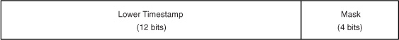
Now that we’ve covered rowkeys, let’s look at how measurements are stored. Notice that the schema contains only a single column family, t. This is because HBase requires a table to contain at least one column family. This table doesn’t use the column family to organize data, but HBase requires one all the same. OpenTSDB uses a 2-byte column qualifier consisting of two parts: the rounded seconds in the first 12 bits and a 4-bit bitmask. The measurement value is stored on 8 bytes in the cell. Figure 7.5 illustrates the column qualifier.

Figure 7.5. Column qualifiers store the final precision of the timestamp as well as a bitmask. The first bit in that mask indicates whether the value in the cell is an integer or a float value.

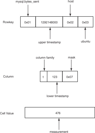
How about an example? Let’s say you’re storing a mysql.bytes_sent metric measurement of 476 observed on Sun, 12 Dec 2010 10:02:03 GMT for the ubuntu host. You previously stored this metric as UID 0x1, the host tag name as 0x2, and the ubuntu tag value as 0x3. The timestamp is represented as a UNIX epoch value of 1292148123. This value is rounded down to the nearest hour and split into 1292148000 and 123. The rowkey and cell as inserted into the tsdb table are shown in figure 7.6. Other measurements collected during the same hour for the same metric on the same host are all stored in other cells in this row.

Figure 7.6. An example rowkey, column qualifier, and cell value storing 476 mysql.bytes_sent at 1292148123 seconds in the tsdb table.

It’s not often we see this kind of bit-wise consideration in Java applications, is it? Much of this is done as a performance optimization. Storing multiple observations per row lets filtered scans disqualify more data in a single exclusion. It also drastically reduces the overall number of rows that must be tracked by the Bloom Filter on rowkey.

Now that you’ve seen the design of an HBase schema, let’s look at how to build a reliable, scalable application using the same methods as those used for OpenTSDB.

7.2.2. Application architecture

While pursuing study of OpenTSDB, it’s useful to keep these HBase design fundamentals in mind:

• Linear scalability over multiple nodes, not a single monolithic server
• Automatic partitioning of data and assignment of partitions
• Strong consistency of data across partitions
• High availability of data services

High availability and linear scalability are frequently primary motivators behind the decision to build on HBase. Often, the application relying on HBase is required to meet these same requirements. Let’s look at how OpenTSDB achieves these goals through its architectural choices. Figure 7.7 provides a view of that architecture.

Figure 7.7. OpenTSDB architecture: separation of concerns. The three areas of concern are data collection, data storage, and serving queries.

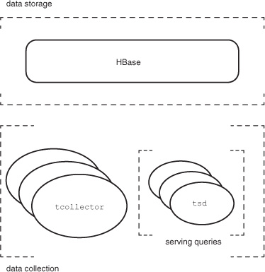
Conceptually speaking, OpenTSDB has three responsibilities: data collection, data storage, and serving queries. As you might guess, data storage is provided by HBase, which already meets these requirements. How does OpenTSDB provide these features for the other responsibilities? Let’s look at them individually, and you’ll see how they’re tied back together through HBase.

Serving Queries

OpenTSDB includes a process called tsd for handling interactions with HBase. It exposes a simple HTTP interface^[2] for serving queries against HBase. Requests can query for either metadata or an image representing the requested time series. All tsd processes are identical and stateless, so high availability is achieved by running multiple tsd machines. Traffic to these machines is routed using a load balancer, just like striping any other HTTP traffic. A client doesn’t suffer from the outage of a single tsd machine because the request is routed to a different one.

² The tsd HTTP API is documented at http://opentsdb.net/http-api.html.

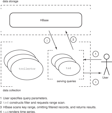
Each query is self-contained and can be answered by a single tsd process independently. This allows OpenTSDB reads to achieve linear scalability. Support for an increasing number of client requests is handled by running more tsd machines. The self-contained nature of the OpenTSDB query has the added bonus of making the results served by tsd cacheable. Figure 7.8 illustrates the OpenTSDB read path.

Figure 7.8. OpenTSDB read path. Requests are routed to an available tsd process that queries HBase and serves the results in the appropriate format.

Data Collection

Data collection requires “boots on the ground,” so to speak. Some process somewhere needs to gather data from the hosts being monitored and store it in HBase. OpenTSDB makes data collection linearly scalable by placing the burden of collection on the hosts being monitored. Each machine runs local processes that collect measurements, and each machine is responsible for sending this data off to OpenTSDB. Adding a new host to your infrastructure places no additional workload exclusively on any individual node in the OpenTSDB cluster.

Network connections time out. Collection services crash. How does OpenTSDB guarantee observation delivery? Attaining high availability, it turns out, is mundane. The tcollector^[3] daemon, also running on each monitored host, takes care of these concerns by gathering measurements locally. It’s responsible for ensuring that observations are delivered to OpenTSDB by waiting out such a network outage. It also manages collection scripts, running them on the appropriate interval or restarting them when they crash. As an added bonus, collection agents written for tcollector can be simple shell scripts.

³tcollector handles other matters as well. More information can be found at http://opentsdb.net/tcollector.html.

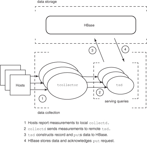
Collector agents don’t write to HBase directly. Doing so would require the tcollector installation to ship an HBase client library along with all its dependencies and configuration. It would also put an unnecessarily large load on HBase. Because the tsd is already deployed to support query load, it’s also used for receiving data. The tsd process exposes a simple telnet-like protocol for receiving observations. It then handles interaction with HBase. The tsd does little work supporting writes, so a small number of tsd instances can handle many times their number in tcollector agents. The OpenTSDB write path is illustrated in figure 7.9.

Figure 7.9. OpenTSDB write path. Collection scripts on monitored hosts report measurements to the local tcollector process. Measurements are then transmitted to a tsd process that handles writing observations to HBase.

You now have a complete view of OpenTSDB. More important, you’ve seen how an application can take advantage of HBase’s strengths. Nothing here should be particularly surprising, especially if you’ve developed a highly available system before. It’s worth noting how much simpler such an application can be when the data-storage system provides these features out of the box. Next, let’s see some code!

7.3. Implementing an HBase application

HBase wants to be used! Notice these interface features directly listed on the HBase home page:

• Easy-to-use Java API for client access
• Thrift gateway and a REST-ful web service that supports XML, Protobuf, and binary data-encoding options
• Query predicate push-down via server-side filters

OpenTSDB’s tsd is implemented in Java but uses an alternative client library called asynchbase^[4] for all interaction, the same asynchbase we covered in depth in chapter 6. To keep the discussion as generally applicable as possible, we’ll present first pseudo-code for HBase interactions and then show you the snippets from OpenTSDB. It’s easier to understand how data is read if you know how it’s written, so this time we’ll begin with the write path.

⁴ For more details, see https://github.com/stumbleupon/asynchbase.

7.3.1. Storing data

As you saw while studying the schema, OpenTSDB stores data in two tables. Before a row can be inserted into the tsdb table, all UIDs must first be generated. Let’s start at the beginning.

Create a UID

Before a measurement can be written to the tsdb table, all of its tags must first be written to tsdb-uid. In pseudo-code, that process is handled by the UniqueId.getOrCreateId() method, which is shown here.

Listing 7.3. Pseudo-code for inserting a tag into the tsdb-uid table

One UniqueId class is instantiated by a tsd process for each kind of UID stored in the table. In this case, metric, tag name, and tag value are the three kinds of UIDs in the system. The local variable kind will be set appropriately in the constructor, along with the variable table for the table name, tsdb-uid by default. The first thing the UniqueId.getOrCreateId() method does is look in the table to see if there’s already a UID of this kind with this name. If it’s there, you’re done. Return it and move on. Otherwise, a new UID needs to be generated and registered for this mapping.

New UIDs are generated by way of a counter stored in this table, increased using the Increment command. A new UID is generated, and the two mappings are stored to the table. Once a mapping is written, it never changes. For this reason, the UID-to-name mapping is written before the name-to-UID mapping. A failure here results in a wasted UID but no further harm. A name-to-UID mapping without its reciprocal means the name is available in the system but can never be resolved from a measurement record. That’s a bad thing because it can lead to orphaned data. Finally, having assigned the bidirectional mapping, the UID is returned.

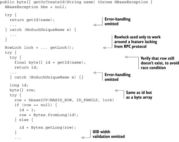
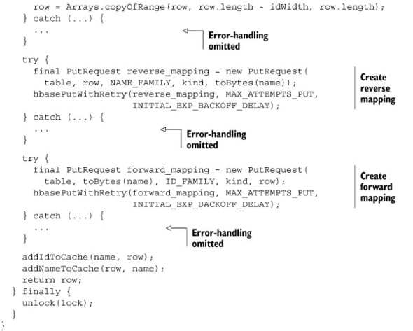
The Java code for this method contains additional complexity due to error handling and a workaround for a feature not yet implemented in the client API. It’s included here but with these additional concerns removed for the sake of brevity.

Listing 7.4. Reduced Java code for UniqueId.getOrCreateId()

Having registered the tags, you can move on to generating a rowkey for an entry in the tsdb table.

Generating a Partial Rowkey

Every rowkey in the tsdb table for the same metric and tag name value pairs looks the same except for the timestamp. OpenTSDB implements this functionality in a helper method for partial construction of these rowkeys in IncomingDataPoints.rowKeyTem-plate(). That method implemented in pseudo-code looks like this.

Listing 7.5. Pseudo-code for generating a rowkey template

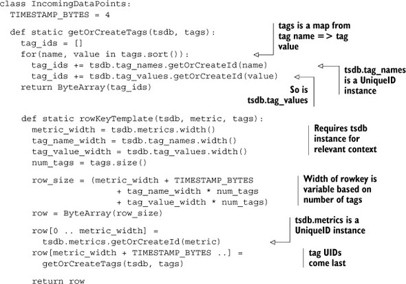
The primary concern of this method is correct placement of the rowkey components. As you saw earlier in figure 7.5, this order is metric UID, partial timestamp, and tag pair UIDs. Notice that the tags are sorted before insertion. This guarantees that the same metric and tags map to the same rowkey every time.

The Java implementation in the following listing is almost identical to the pseudo-code in listing 7.5. The biggest difference is organization of helper methods.

Listing 7.6. Java code for IncomingDataPoints.rowKeyTemplate()

static byte[] rowKeyTemplate(final TSDB tsdb,
                             final String metric,
                             final Map<String, String> tags) {
  final short metric_width = tsdb.metrics.width();
  final short tag_name_width = tsdb.tag_names.width();
  final short tag_value_width = tsdb.tag_values.width();
  final short num_tags = (short) tags.size();

  int row_size = (metric_width + Const.TIMESTAMP_BYTES
                  + tag_name_width * num_tags
                  + tag_value_width * num_tags);
  final byte[] row = new byte[row_size];

  short pos = 0;

  copyInRowKey(row, pos, (AUTO_METRIC ? tsdb.metrics.getOrCreateId(metric)
                     : tsdb.metrics.getId(metric)));
  pos += metric_width;

  pos += Const.TIMESTAMP_BYTES;

  for(final byte[] tag : Tags.resolveOrCreateAll(tsdb, tags)) {
    copyInRowKey(row, pos, tag);
    pos += tag.length;
  }
  return row;
}

That’s all there is to it! You now have all the pieces.

Writing a Measurement

With all the necessary helper methods in place, it’s time to write a record to the tsdb table. The process looks like this:

1. Build the rowkey.
2. Decide on the column family and qualifier.
3. Identify the bytes to store in the cell.
4. Write the record.

This logic is encapsulated in the TSDB.addPoint() method. Those tsdb instances in the previous code listings are instances of this class. Let’s start once more with pseudo-code before diving into the Java implementation.

Listing 7.7. Pseudo-code for inserting a tsdb record

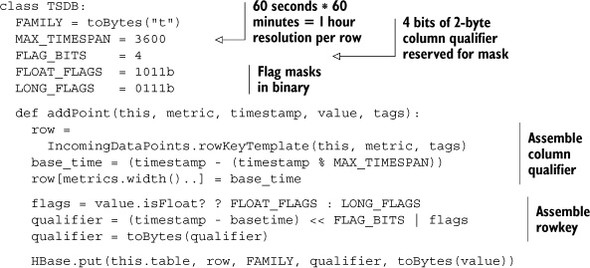
Writing the value is as simple as that! Now let’s look at the same thing in Java. The code for writing Longs and Floats is almost identical. We’ll look at writing Longs.

Listing 7.8. Java code for TSDB.addPoint()

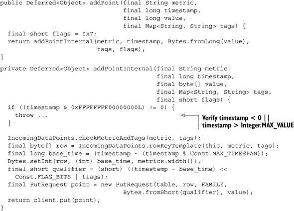
Looking back over these listings, both pseudo-code and Java, there’s not much interaction with HBase going on. The most complicated part of writing a row to HBase is assembling the values you want to write. Writing the record is the easy part!

OpenTSDB goes to great lengths to assemble a rowkey. Those efforts are well rewarded at read time. The next section shows you how.

7.3.2. Querying data

With data stored in HBase, it’s useful to pull it out again. OpenTSDB does this for two distinct use cases: UID name auto-completion and querying time series. In both cases, the sequence of steps is identical:

1. Identify a rowkey range.
2. Define applicable filter criteria.
3. Execute the scan.

Let’s see what it takes to implement auto-complete for time-series metadata.

UID Name Auto-Completion

Do you remember the bidirectional mapping in the tsdb-uid table? The reverse mapping is used in support of the auto-completion UI feature shown in figure 7.10.

Figure 7.10. OpenTSDB metric auto-completion is supported by the name-to-UID mapping stored in the tsdb-uid table.

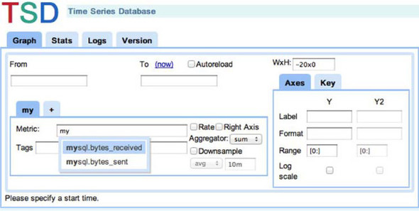
HBase supports this application feature with the rowkey scan pattern of data access. HBase keeps an index over the rowkeys in each table so locating the starting point is very fast. From there, the HBase BlockCache takes over, rapidly reading consecutive blocks from memory and off the HDFS when necessary. In this case, those consecutive blocks contain rows in the tsdb-uid table. In figure 7.10, the user entered my in the Metric field. These characters are taken as the start row of the scan. You want to display entries matching only this prefix, so the end row of the scan is calculated to be mz. You also only want records where the id column family is populated; otherwise you’ll interpret UIDs as text. The Java code is readable, so we’ll skip the pseudo-code.

Listing 7.9. Creating a scanner over tsdb-uid in UniqueId.getSuggestScanner()

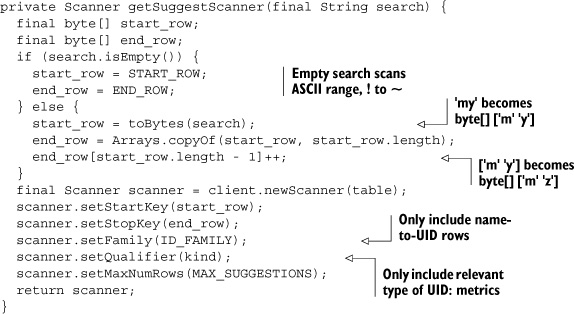
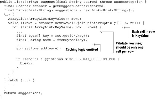
With a scanner constructed, consuming records out of HBase is like reading any other iterator. Reading suggestions off the scanner is a matter of extracting the byte array and interpreting it as a string. Lists are used to maintain the sorted order of returned results. Here’s the Java code, again reduced of ancillary concerns.

Listing 7.10. Reduced Java code for UniqueId.suggest()

Reading Time Series

The same technique is used to read segments of time-series data from the tsdb table. The query is more complex because this table’s rowkey is more complex than tsdbuid. That complexity comes by way of the multifield filter. Against this table, metric, date range, and tags are all considered in the filter. That filter is applied on the HBase servers, not on the client. That detail is crucial because it drastically reduces the amount of data transferred to the tsd client. Keep in mind that this is a regex over the un-interpreted bytes in the rowkey.

The other primary difference between this scan and the previous example is time-series aggregation. The OpenTSDB UI allows multiple time series over common tags to be aggregated into a single time series for display. These groups of tags must also be considered while building the filter. TsdbQuery maintains private variables named group_bys and group_by_values for this purpose.

All this filter business is implemented through the TsdbQuery.run() method. This method works just like before, creating a filtered scanner, iterating over the returned rows, and gathering data to display. Helper methods TsdbQuery.getScanner() and TsdbQuery.findSpans() are almost identical to UniqueId.getSuggestScanner() and UniqueId.suggest(), respectively; their listings are omitted. Instead, look at TsdbQuery.createAndSetFilter() in the following listing. It handles the interesting part of setting up a regular expression filter over the rowkeys.

Listing 7.11. Java code for TsdbQuery.createAndSetFilter()

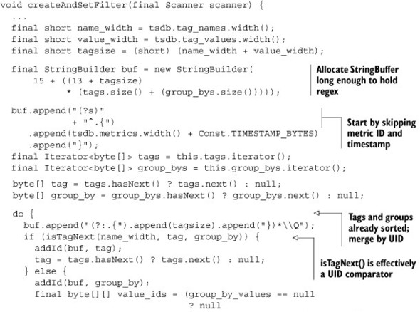
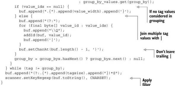
Building a byte-wise regular expression isn’t as scary as it sounds. With this filter in place, OpenTSDB submits the query to HBase. Each node in the cluster hosting data between the start and end keys handles its portion of the scan, filtering relevant records. The resulting rows are sent back to tsd for rendering. Finally, you see your graph on the other end.

7.4. Summary

Earlier we said that HBase is a flexible, scalable, accessible database. You’ve just seen some of that in action. A flexible data model allows HBase to store all manner of data, time-series being just one example. HBase is designed for scale, and now you’ve seen how to design an application to scale right along with it. You also have some insight into how to use the API. We hope the idea of building against HBase is no longer so daunting. We’ll continue exploring building real-world applications on HBase in the next chapter.