Chapter 3. Distributed HBase, HDFS, and MapReduce

 

 

As you’ve realized, HBase is built on Apache Hadoop. What may not yet be clear to you is why. Most important, what benefits do we, as application developers, enjoy from this relationship? HBase depends on Hadoop for two separate concerns. Hadoop MapReduce provides a distributed computation framework for high-throughput data access. The Hadoop Distributed File System (HDFS) gives HBase a storage layer providing availability and reliability. In this chapter, you’ll see how Twit-Base is able to take advantage of this data access for bulk processing and how HBase uses HDFS to guarantee availability and reliability.

To begin this chapter, we’ll show you why MapReduce is a valuable alternative access pattern for processing data in HBase. Then we’ll describe Hadoop MapReduce in general. With this knowledge, we’ll tie it all back into HBase as a distributed system. We’ll show you how to use HBase from MapReduce jobs and explain some useful tricks you can do with HBase from MapReduce. Finally, we’ll show you how HBase provides availability, reliability, and durability for your data. If you’re a seasoned Hadooper and know a bunch about MapReduce and HDFS, you can jump straight to section 3.3 and dive into learning about distributed HBase.

The code used in this chapter is a continuation of the TwitBase project started in the previous chapter and is available at https://github.com/hbaseinaction/twitbase.

3.1. A case for MapReduce

Everything you’ve seen so far about HBase has a focus on online operations. You expect every Get and Put to return results in milliseconds. You carefully craft your Scans to transfer as little data as possible over the wire so they’ll complete as quickly as possible. You emphasize this behavior in your schema designs, too. The twits table’s rowkey is designed to maximize physical data locality and minimize the time spent scanning records.

Not all computation must be performed online. For some applications, offline operations are fine. You likely don’t care if the monthly site traffic summary report is generated in four hours or five hours, as long as it completes before the business owners are ready for it. Offline operations have performance concerns as well. Instead of focusing on individual request latency, these concerns often focus on the entire computation in aggregate. MapReduce is a computing paradigm built for offline (or batch) processing of large amounts of data in an efficient manner.

3.1.1. Latency vs. throughput

The concept of this duality between online and offline concerns has come up a couple times now. This duality exists in traditional relational systems too, with Online Transaction Processing (OLTP) and Online Analytical Processing (OLAP). Different database systems are optimized for different access patterns. To get the best performance for the least cost, you need to use the right tool for the job. The same system that handles fast real-time queries isn’t necessarily optimized for batch operations on large amounts of data.

Consider the last time you needed to buy groceries. Did you go to the store, buy a single item, and return it to your pantry, only to return to the store for the next item? Well sure, you may do this sometimes, but it’s not ideal, right? More likely you made a shopping list, went to the store, filled up your cart, and brought everything home. The entire trip took longer, but the time you spent away from home was shorter per item than taking an entire trip per item. In this example, the time in transit dominates the time spent shopping for, purchasing, and unpacking the groceries. When buying multiple things at once, the average time spent per item purchased is much lower. Making the shopping list results in higher throughput. While in the store, you’ll need a bigger cart to accommodate that long shopping list; a small hand basket won’t cut it. Tools that work for one approach aren’t always sufficient for another.

We think about data access in much the same way. Online systems focus on minimizing the time it takes to access one piece of data—the round trip of going to the store to buy a single item. Response latency measured on the 95th percentile is generally the most important metric for online performance. Offline systems are optimized for access in the aggregate, processing as much as we can all at once in order to maximize throughput. These systems usually report their performance in number of units processed per second. Those units might be requests, records, or megabytes. Regardless of the unit, it’s about overall processing time of the task, not the time of an individual unit.

3.1.2. Serial execution has limited throughput

You wrapped up the last chapter by using Scan to look at the most recent twits for a user of TwitBase. Create the start rowkey, create the end rowkey, and execute the scan. That works for exploring a single user, but what if you want to calculate a statistic over all users? Given your user base, perhaps it would be interesting to know what percentage of twits are about Shakespeare. Maybe you’d like to know how many users have mentioned Hamlet in their twits.

How can you look at all the twits from all the users in the system to produce these metrics? The Scan object will let you do that:

HTableInterface twits = pool.getTable(TABLE_NAME);
Scan s = new Scan();
ResultScanner results = twits.getScanner(s);
for(Result r : results) {
  ... // process twits
}

This block of code asks for all the data in the table and returns it for your client to iterate through. Does it have a bit of code-smell to you? Even before we explain the inner workings of iterating over the items in the ResultScanner instance, your intuition should flag this as a bad idea. Even if the machine running this loop could process 10 MB/sec, churning through 100 GB of twits would take nearly 3 hours!

3.1.3. Improved throughput with parallel execution

What if you could parallelize this problem—that is, split your gigabyte of twits into pieces and process all the pieces in parallel? You could turn 3 hours into 25 minutes by spinning up 8 threads and running them all in parallel. A laptop has 8 cores and can easily hold 100 GB of data, so assuming it doesn’t run out of memory, this should be pretty easy.

 

 

The code for distributing the work over different threads might look something like this:

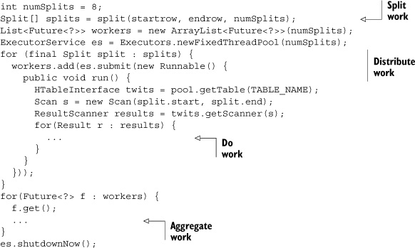
That’s not bad, but there’s one problem. People are using TwitBase, and before long you’ll have 200 GB of twits—and then 1 TB and then 50 TB! Fitting all that data on your laptop’s hard drive is a serious challenge, and it’s running desperately low on cores. What do you do? You can settle for waiting longer for the computation to finish, but that solution won’t last forever as hours quickly turn into days. Parallelizing the computation worked well last time, so you might as well throw more computers at it. Maybe you can buy 20 cheapish servers for the price of 10 fancy laptops.

Now that you have the computing power, you still need to deal with splitting the problem across those machines. Once you’ve solved that problem, the aggregation step will require a similar solution. And all this while you’ve assumed everything works as expected. What happens if a thread gets stuck or dies? What if a hard drive fails or the machine suffers random RAM corruption? It would be nice if the workers could restart where they left off in case one of the splits kills the program. How does the aggregation keep track of which splits have finished and which haven’t? How do the results get shipped back for aggregation? Parallelizing the problem was pretty easy, but the rest of this distributed computation is painful bookkeeping. If you think about it, the bookkeeping would be required for every algorithm you write. The solution is to make that into a framework.

3.1.4. MapReduce: maximum throughput with distributed parallelism

Enter Hadoop. Hadoop gives us two major components that solve this problem. The Hadoop Distributed File System (HDFS) gives all these computers a common, shared file system where they can all access the data. This removes a lot of the pain from farming out the data to the workers and aggregating the work results. Your workers can access the input data from HDFS and write out the processed results to HDFS, and all the others can see them. Hadoop MapReduce does all the bookkeeping we described, splitting up the workload and making sure it gets done. Using MapReduce, all you write are the Do Work and Aggregate Work bits; Hadoop handles the rest. Hadoop refers to the Do Work part as the Map Step. Likewise, Aggregate Work is the Reduce Step. Using Hadoop MapReduce, you have something like this instead:

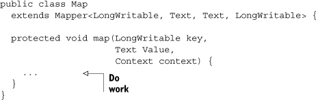
This code implements the map task. This function expects long keys and Text instances as input and writes out pairs of Text to LongWritable. Text and LongWritable are Hadoop-speak for String and Long, respectively.

Notice all the code you’re not writing. There are no split calculations, no Futures to track, and no thread pool to clean up after. Better still, this code can run anywhere on the Hadoop cluster! Hadoop distributes your worker logic around the cluster according to resource availability. Hadoop makes sure every machine receives a unique slice of the twits table. Hadoop ensures no work is left behind, even if workers crash.

Your Aggregate Work code is shipped around the cluster in a similar fashion. The Hadoop harness looks something like this:

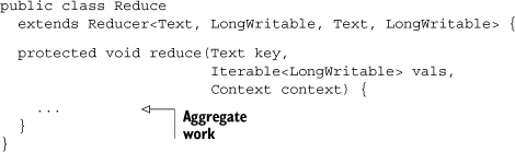
Here you see the reduce task. The function receives the [String,Long] pairs output from map and produces new [String,Long] pairs. Hadoop also handles collecting the output. In this case, the [String,Long] pairs are written back to the HDFS. You could have just as easily written them back to HBase. HBase provides TableMapper and TableReducer classes to help with that.

You’ve just seen when and why you’ll want to use MapReduce instead of programming directly against the HBase client API. Now let’s take a quick look at the Map-Reduce framework. If you’re already familiar with Hadoop MapReduce, feel free to skip down to section 3.3: “HBase in distributed mode.”

3.2. An overview of Hadoop MapReduce

In order to provide you with a general-purpose, reliable, fault-tolerant distributed computation harness, MapReduce constrains how you implement your program. These constraints are as follows:

• All computations are implemented as either map or reduce tasks.
• Each task operates over a portion of the total input data.
• Tasks are defined primarily in terms of their input data and output data.
• Tasks depend on their input data and don’t communicate with other tasks.

Hadoop MapReduce enforces these constraints by requiring that programs be implemented with map and reduce functions. These functions are composed into a Job and run as a unit: first the mappers and then the reducers. Hadoop runs as many simultaneous tasks as it’s able. Because there are no runtime dependencies between concurrent tasks, Hadoop can run them in any order as long as the map tasks are run before the reduce tasks. The decisions of how many tasks to run and which tasks to run are up to Hadoop.

 

 

3.2.1. MapReduce data flow explained

Implementing programs in terms of Map and Reduce Steps requires a change in how you tackle a problem. This can be quite an adjustment for developers accustomed to other common kinds of programming. Some people find this change so fundamental that they consider it a change of paradigm. Don’t worry! This claim may or may not be true. We’ll make it as easy as possible to think in MapReduce. MapReduce is all about processing large amounts of data in parallel, so let’s break down a MapReduce problem in terms of the flow of data.

For this example, let’s consider a log file from an application server. Such a file contains information about how a user spends time using the application. Its contents look like this:

Date        Time   UserID Activity    TimeSpent

01/01/2011  18:00  user1  load_page1  3s
01/01/2011  18:01  user1  load_page2  5s
01/01/2011  18:01  user2  load_page1  2s
01/01/2011  18:01  user3  load_page1  3s
01/01/2011  18:04  user4  load_page3  10s
01/01/2011  18:05  user1  load_page3  5s
01/01/2011  18:05  user3  load_page5  3s
01/01/2011  18:06  user4  load_page4  6s
01/01/2011  18:06  user1  purchase    5s
01/01/2011  18:10  user4  purchase    8s
01/01/2011  18:10  user1  confirm     9s
01/01/2011  18:10  user4  confirm     11s
01/01/2011  18:11  user1  load_page3  3s

Let’s calculate the amount of time each user spends using the application. A basic implementation might be to iterate through the file, summing the values of TimeSpent for each user. Your program could have a single HashMap (or dict, for you Pythonistas) with UserID as the key and summed TimeSpent as the value. In simple pseudo-code, that program might look like this:

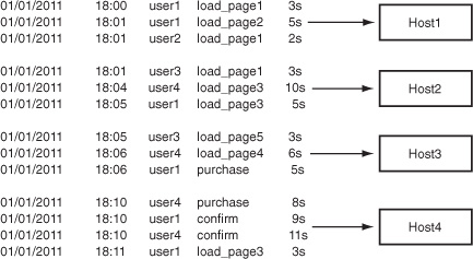
This looks a lot like the serial example from the previous section, doesn’t it? Like the serial example, its throughput is limited to a single thread on a single machine. MapReduce is for distributed parallelism. The first thing to do when parallelizing a problem is break it up. Notice that each line in the input file is processed independently from all the other lines. The only time when data from different lines is seen together is during the aggregation step. That means this input file can be parallelized by any number of lines, processed independently, and aggregated to produce exactly the same result. Let’s split it into four pieces and assign those pieces to four different machines, as per figure 3.1.

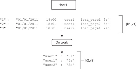
Figure 3.1. Splitting and assigning work. Each record in the log file can be processed independently, so you split the input file according to the number of workers available.

Look closely at these divisions. Hadoop doesn’t know anything about this data other than that it’s line-oriented. In particular, there’s no effort made to group according to UserID. This is an important point we’ll address shortly.

Now the work is divided and assigned. How do you rewrite the program to work with this data? As you saw from the map and reduce stubs, MapReduce operates in terms of key-value pairs. For line-oriented data like this, Hadoop provides pairs of [line number:line]. While walking through the MapReduce workflow, we refer in general to this first set of key-value pairs as [k1,v1]. Let’s start by writing the Map Step, again in pseudo-code:

The Map Step is defined in terms of the lines from the file. For each line in its portion of the file, this Map Step splits the line and produces a new key-value pair of [UserID:TimeSpent]. In this pseudo-code, the function emit handles reporting the produced pairs back to Hadoop. As you likely guessed, we’ll refer to the second set of key-value pairs as [k2,v2]. Figure 3.2 continues where the previous figure left off.

Figure 3.2. Do work. The data assigned to Host1, [k1,v1], is passed to the Map Step as pairs of line number to line. The Map Step processes each line and produces pairs of UserID to TimeSpent, [k2,v2].

Before Hadoop can pass the values of [k2,v2] on to the Reduce Step, a little bookkeeping is necessary. Remember that bit about grouping by UserID? The Reduce Step expects to operate over all TimeSpent by a given UserID. For this to happen correctly, that grouping work happens now. Hadoop calls these the Shuffle and Sort Steps. Figure 3.3 illustrates these steps.

Figure 3.3. Hadoop performs the Shuffle and Sort Step automatically. It serves to prepare the output from the Map Step for aggregation in the Reduce Step. No values are changed by the process; it serves only to reorganize data.

MapReduce takes [k2,v2], the output from all four Map Steps on all four servers, and assigns it to reducers. Each reducer is assigned a set of values of UserID and it copies those [k2,v2] pairs from the mapper nodes. This is called the Shuffle Step. A reduce task expects to process all values of k2 at the same time, so a sort on key is necessary. The output of that Sort Step is [k2,<v2>], a list of Times for each UserID. With the grouping complete, the reduce tasks run. The aggregate work function looks like this:

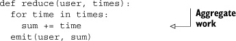
The Reduce Step processes the [k2,<v2>] input and produces aggregated work as pairs of [UserID:TotalTime]. These sums are collected by Hadoop and written to the output destination. Figure 3.4 illustrates this final step.

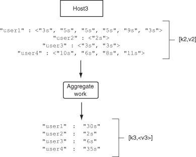
Figure 3.4. Aggregate work. Available servers process the groups of UserID to Times, [k2,<v2>], in this case, summing the values. Final results are emitted back to Hadoop.

You can run this application if you’d like; the source is bundled with the TwitBase code. To do so, compile the application JAR and launch the job like this:

$ mvn clean package
[INFO] Scanning for projects...
[INFO]
[INFO] ---------------------------------------------------------------
[INFO] Building TwitBase 1.0.0
[INFO] ---------------------------------------------------------------
...
[INFO] ---------------------------------------------------------------
[INFO] BUILD SUCCESS
[INFO] ---------------------------------------------------------------
$ java -cp target/twitbase-1.0.0.jar 
  HBaseIA.TwitBase.mapreduce.TimeSpent 
  src/test/resource/listing 3.3.txt ./out
...
22:53:15 INFO mapred.JobClient: Running job: job_local_0001
22:53:15 INFO mapred.Task:  Using ResourceCalculatorPlugin : null
22:53:15 INFO mapred.MapTask: io.sort.mb = 100
22:53:15 INFO mapred.MapTask: data buffer = 79691776/99614720
22:53:15 INFO mapred.MapTask: record buffer = 262144/327680
22:53:15 INFO mapred.MapTask: Starting flush of map output
22:53:15 INFO mapred.MapTask: Finished spill 0
22:53:15 INFO mapred.Task: Task:attempt_local_0001_m_000000_0 is done. And is
     in the process of commiting
22:53:16 INFO mapred.JobClient:  map 0% reduce 0%
...

22:53:21 INFO mapred.Task: Task 'attempt_local_0001_r_000000_0' done.
22:53:22 INFO mapred.JobClient:  map 100% reduce 100%
22:53:22 INFO mapred.JobClient: Job complete: job_local_0001
$ cat out/part-r-00000
user1    30
user2    2
user3    6
user4    35

That’s MapReduce as the data flows. Every MapReduce application performs this sequence of steps, or most of them. If you can follow these basic steps, you’ve successfully grasped this new paradigm.

3.2.2. MapReduce under the hood

Building a system for general-purpose, distributed, parallel computation is nontrivial. That’s precisely why we leave that problem up to Hadoop! All the same, it can be useful to understand how things are implemented, particularly when you’re tracking down a bug. As you know, Hadoop MapReduce is a distributed system. Several independent components form the framework. Let’s walk through them and see what makes MapReduce tick.

A process called the JobTracker acts as an overseer application. It’s responsible for managing the MapReduce applications that run on your cluster. Jobs are submitted to the JobTracker for execution and it manages distributing the workload. It also keeps tabs on all portions of the job, ensuring that failed tasks are retried. A single Hadoop cluster can run multiple MapReduce applications simultaneously. It falls to the Job-Tracker to oversee resource utilization, and job scheduling as well.

The work defined by the Map Step and Reduce Step is executed by another process called the TaskTracker. Figure 3.5 illustrates the relationship between a Job-Tracker and its TaskTrackers. These are the actual worker processes. An individual TaskTracker isn’t specialized in any way. Any TaskTracker can run any task, be it a map or reduce, from any job. Hadoop is smart and doesn’t randomly spray work across the nodes. As we mentioned, Hadoop is optimized for minimal network I/O. It achieves this by bringing computation as close as possible to the data. In a typical Hadoop, HDFS DataNodes and MapReduce TaskTrackers are collocated with each other. This allows the map and reduce tasks to run on the same physical node where the data is located. By doing so, Hadoop can avoid transferring the data over the network. When it isn’t possible to run the tasks on the same physical node, running the task in the same rack is a better choice than running it on a different rack. When HBase comes into the picture, the same concepts apply, but in general HBase deployments look different from standard Hadoop deployments. You’ll learn about deployment strategies in chapter 10.

Figure 3.5. The JobTracker and its TaskTrackers are responsible for execution of the MapReduce applications submitted to the cluster.

3.3. HBase in distributed mode

By now you know that HBase is essentially a database built on top of HDFS. It’s also sometimes referred to as the Hadoop Database, and that’s where it got its name. Theoretically, HBase can work on top of any distributed file system. It’s just that it’s tightly integrated with HDFS, and a lot more development effort has gone into making it work well with HDFS as compared to other distributed file systems. Having said that, from a theoretical standpoint, there is no reason that other file systems can’t support HBase. One of the key factors that makes HBase scalable (and fault tolerant) is that it persists its data onto a distributed file system that provides it a single namespace. This is one of the key factors that allows HBase to be a fully consistent data store.

HDFS is inherently a scalable store, but that’s not enough to scale HBase as a low-latency data store. There are other factors at play that you’ll learn about in this section. Having a good understanding of these is important in order to design your application optimally. This knowledge will enable you to make smart choices about how you want to access HBase, what your keys should look like, and, to some degree, how HBase should be configured. Configuration isn’t something you as an application developer should be worried about, but it’s likely that you’ll have some role to play when bringing HBase into your stack initially.

3.3.1. Splitting and distributing big tables

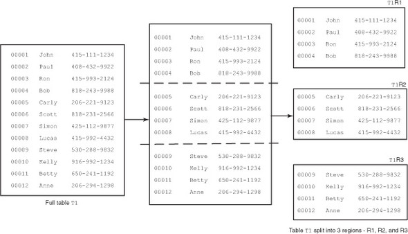
Just as in any other database, tables in HBase comprise rows and columns, albeit with a different kind of schema. Tables in HBase can scale to billions of rows and millions of columns. The size of each table can run into terabytes and sometimes even petabytes. It’s clear at that scale that the entire table can’t be hosted on a single machine. Instead, tables are split into smaller chunks that are distributed across multiple servers. These smaller chunks are called regions (figure 3.6). Servers that host regions are called RegionServers.

Figure 3.6. A table consists of multiple smaller chunks called regions.

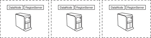
RegionServers are typically collocated with HDFS DataNodes (figure 3.7) on the same physical hardware, although that’s not a requirement. The only requirement is that RegionServers should be able to access HDFS. They’re essentially clients and store/access data on HDFS. The master process does the distribution of regions among RegionServers, and each RegionServer typically hosts multiple regions.

Figure 3.7. HBase RegionServer and HDFS DataNode processes are typically collocated on the same host.

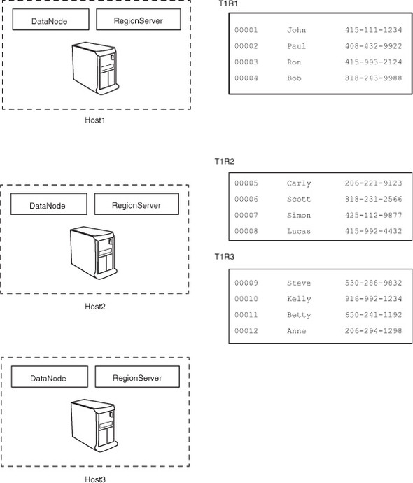
Given that the underlying data is stored in HDFS, which is available to all clients as a single namespace, all RegionServers have access to the same persisted files in the file system and can therefore host any region (figure 3.8). By physically collocating Data-Nodes and RegionServers, you can use the data locality property; that is, RegionServers can theoretically read and write to the local DataNode as the primary DataNode.

Figure 3.8. Any RegionServer can host any region. RegionServers 1 and 2 are hosting regions, whereas RegionServer 3 isn’t.

You may wonder where the TaskTrackers are in this scheme of things. In some HBase deployments, the MapReduce framework isn’t deployed at all if the workload is primarily random reads and writes. In other deployments, where the MapReduce processing is also a part of the workloads, TaskTrackers, DataNodes, and HBase Region-Servers can run together.

The size of individual regions is governed by the configuration parameter hbase.hregion.max.filesize, which can be configured in the hbase-site.xml file of your deployment. When a region becomes bigger than that size (as you write more data into it), it gets split into two regions.

3.3.2. How do I find my region?

You’ve learned that tables are split into regions and regions are assigned to Region-Servers without any predefined assignment rules. In case you’re wondering, regions don’t keep moving around in a running system! Region assignment happens when regions split (as they grow in size), when RegionServers die, or when new RegionServers are added to the deployment. An important question to ask here is, “When a region is assigned to a RegionServer, how does my client application (the one doing reads and writes) know its location?”

Two special tables in HBase, -ROOT- and .META., help find where regions for various tables are hosted. Like all tables in HBase, -ROOT- and .META. are also split into regions. -ROOT- and .META. are both special tables, but -ROOT- is more special than .META.; -ROOT- never splits into more than one region. .META. behaves like all other tables and can split into as many regions as required.

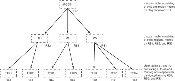
When a client application wants to access a particular row, it goes to the -ROOT- table and asks it where it can find the region responsible for that particular row. -ROOT- points it to the region of the .META. table that contains the answer to that question. The .META. table consists of entries that the client application uses to determine which RegionServer is hosting the region in question. Think of this like a distributed B+Tree of height 3 (see figure 3.9). The -ROOT- table is the -ROOT- node of the B+Tree. The .META. regions are the children of the -ROOT- node (-ROOT-region)n and the regions of the user tables (leaf nodes of the B+Tree) are the children of the .META. regions.

Figure 3.9. -ROOT-, .META., and user tables viewed as a B+Tree

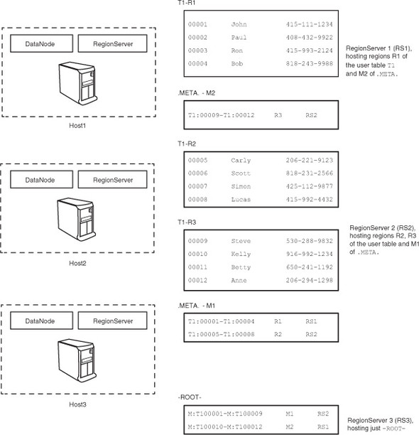
Let’s put -ROOT- and .META. into the example; see figure 3.10. Note that the region assignments shown here are arbitrary and don’t represent how they will happen when such a system is deployed.

Figure 3.10. User table T1 in HBase, along with -ROOT- and .META., distributed across the various RegionServers

3.3.3. How do I find the -ROOT- table?

You just learned how the -ROOT- and .META. tables help you find out other regions in the system. At this point, you might be left with a question: “Where is the -ROOT-table?” Let’s figure that out now.

The entry point for an HBase system is provided by another system called ZooKeeper (http://zookeeper.apache.org/). As stated on ZooKeeper’s website, ZooKeeper is a centralized service for maintaining configuration information, naming, providing distributed synchronization, and providing group services. It’s a highly available, reliable distributed configuration service. Just as HBase is modeled after Google’s BigTable, ZooKeeper is modeled after Google’s Chubby.^[1]

¹ Mike Burrow, “The Chubby Lock Service for Loosely-Coupled Distributed Systems,” Google Research Publications, http://research.google.com/archive/chubby.html.

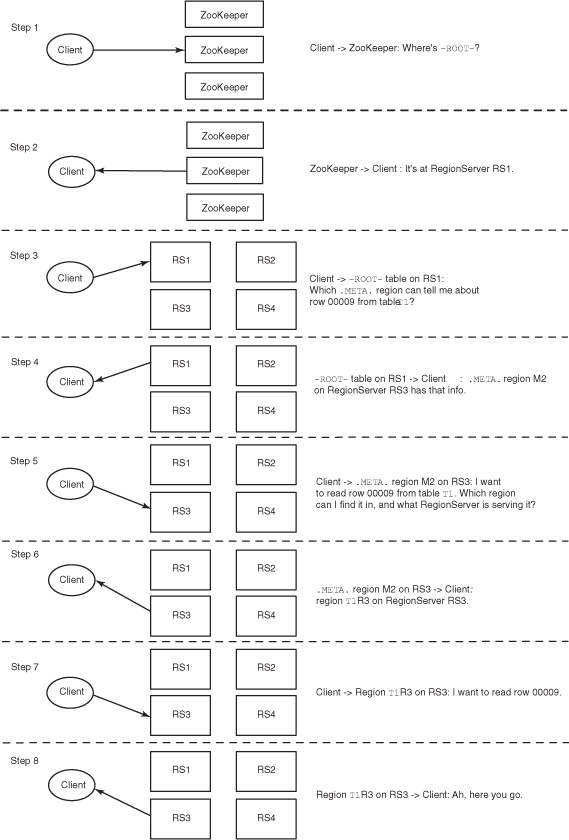
The client interaction with the system happens in steps, where ZooKeeper is the point of entry, as mentioned earlier. These steps are highlighted in figure 3.11.

Figure 3.11. Steps that take place when a client interacts with an HBase system. The interaction starts with ZooKeeper and goes to the RegionServer serving the region with which the client needs to interact. The interaction with the RegionServer could be for reads or writes. The information about -ROOT- and .META. is cached by the client for future interactions and is refreshed if the regions it’s expecting to interact with based on that information don’t exist on the node it thinks they should be on.

This section gave you an overview of the implementation of HBase’s distributed architecture. You can see all these details for yourself on your own cluster. We show you exactly how to explore ZooKeeper, -ROOT-, and .META. in appendix A.

3.4. HBase and MapReduce

Now that you have an understanding of MapReduce and HBase in distributed mode, let’s look at them together. There are three different ways of interacting with HBase from a MapReduce application. HBase can be used as a data source at the beginning of a job, as a data sink at the end of a job, or as a shared resource for your tasks. None of these modes of interaction are particularly mysterious. The third, however, has some interesting use cases we’ll address shortly.

All the code snippets used in this section are examples of using the Hadoop MapReduce API. There are no HBase client HTable or HTablePool instances involved. Those are embedded in the special input and output formats you’ll use here. You will, however, use the Put, Delete, and Scan objects with which you’re already familiar. Creating and configuring the Hadoop Job and Configuration instances can be messy work. These snippets emphasize the HBase portion of that work. You’ll see a full working example in section 3.5.

3.4.1. HBase as a source

In the example MapReduce application, you read lines from log files sitting in the HDFS. Those files, specifically the directory in HDFS containing those files, act as the data source for the MapReduce job. The schema of that data source describes [k1,v1] tuples as [line number:line]. The TextInputFormat class configured as part of the job defines this schema. The relevant code from the TimeSpent example looks like this:

Configuration conf = new Configuration();
Job job = new Job(conf, "TimeSpent");
...
job.setInputFormatClass(TextInputFormat.class);
job.setOutputFormatClass(TextOutputFormat.class);

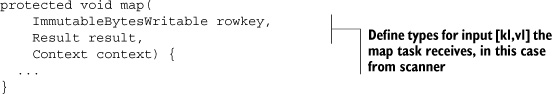
TextInputFormat defines the [k1,v1] type for line number and line as the types LongWritable and Text, respectively. LongWritable and Text are serializable Hadoop wrapper types over Java’s Long and String. The associated map task definition is typed for consuming these input pairs:

public void map(LongWritable key, Text value,
Context context) {
  ...
}

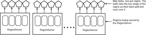
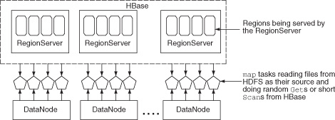
HBase provides similar classes for consuming data out of a table. When mapping over data in HBase, you use the same Scan class you used before. Under the hood, the row-range defined by the Scan is broken into pieces and distributed to all the workers (figure 3.12).

Figure 3.12. MapReduce job with mappers taking regions from HBase as their input source. By default, one mapper is created per region.

This is identical to the splitting you saw in figure 3.1. Creating a Scan instance for scanning over all rows in a table from MapReduce looks like this:

Scan scan = new Scan();
scan.addColumn(Bytes.toBytes("twits"), Bytes.toBytes("twit"));

In this case, you’re asking the scanner to return only the text from the twits table.

Just like consuming text lines, consuming HBase rows requires a schema. All jobs reading from an HBase table accept their [k1,v1] pairs in the form of [rowkey:scan result]. That’s the same scanner result as when you consume the regular HBase API. They’re presented using the types ImmutableBytesWritable and Result. The provided TableMapper wraps up these details for you, so you’ll want to use it as the base class for your Map Step implementation:

The next step is to take your Scan instance and wire it into MapReduce. HBase provides the handy TableMapReduceUtil class to help you initialize the Job instance:

TableMapReduceUtil.initTableMapperJob(
  "twits",
  scan,
  Map.class,
  ImmutableBytesWritable.class,
  Result.class,
  job);

This takes your job-configuration object and sets up the HBase-specific input format (TableInputFormat). It then configures MapReduce to read from the table using your Scan instance. It also wires in your Map and Reduce class implementations. From here, you write and run the MapReduce application as normal.

When you run a MapReduce job as described here, one map task is launched for every region in the HBase table. In other words, the map tasks are partitioned such that each map task reads from a region independently. The JobTracker tries to schedule map tasks as close to the regions as possibly and take advantage of data locality.

3.4.2. HBase as a sink

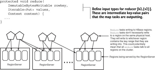
Writing to an HBase table from MapReduce (figure 3.13) as a data sink is similar to reading from a table in terms of implementation.

Figure 3.13. HBase as a sink for a MapReduce job. In this case, the reduce tasks are writing to HBase.

HBase provides similar tooling to simplify the configuration. Let’s first make an example of sink configuration in a standard MapReduce application.

In TimeSpent, the values of [k3,v3] generated by the aggregators are [UserID:TotalTime]. In the MapReduce application, they’re of the Hadoop serializable types Text and LongWritable, respectively. Configuring output types is similar to configuring input types, with the exception that the [k3,v3] output types can’t be inferred by the OutputFormat:

Configuration conf = new Configuration();
Job job = new Job(conf, "TimeSpent");
job.setOutputKeyClass(Text.class);
job.setOutputValueClass(LongWritable.class);
...
job.setInputFormatClass(TextInputFormat.class);
job.setOutputFormatClass(TextOutputFormat.class);

In this case, no line numbers are specified. Instead, the TextOuputFormat schema creates a tab-separated output file containing first the UserID and then the TotalTime. What’s written to disk is the String representation of both types.

The Context object contains the type information. The reduce function is defined as

public void reduce(Text key, Iterable<LongWritable> values,
Context context) {
  ...
}

When writing to HBase from MapReduce, you’re again using the regular HBase API. The types of [k3,v3] are assumed to be a rowkey and an object for manipulating HBase. That means the values of v3 must be either Puts or Deletes. Because both of these object types include the relevant rowkey, the value of k3 is ignored. Just as the TableMapper wraps up these details for you, so does the TableReducer:

The last step is wiring your reducer into the job configuration. You need to specify the destination table along with all the appropriate types. Once again, it’s TableMapReduceUtil to the rescue; it sets up the TableOutputFormat for you! You use IdentityTableReducer, a provided class, because you don’t need to perform any computation in the Reduce Step:

TableMapReduceUtil.initTableReducerJob(
  "users",
  IdentityTableReducer.class,
  job);

Now your job is completely wired up, and you can proceed as normal. Unlike the case where map tasks are reading from HBase, tasks don’t necessarily write to a single region. The writes go to the region that is responsible for the rowkey that is being written by the reduce task. The default partitioner that assigns the intermediate keys to the reduce tasks doesn’t have knowledge of the regions and the nodes that are hosting them and therefore can’t intelligently assign work to the reducers such that they write to the local regions. Moreover, depending on the logic you write in the reduce task, which doesn’t have to be the identity reducer, you might end up writing all over the table.

3.4.3. HBase as a shared resource

Reading from and writing to HBase using MapReduce is handy. It gives us a harness for batch processing over data in HBase. A few predefined MapReduce jobs ship with HBase; you can explore their source for more examples of using HBase from Map-Reduce. But what else can you do with HBase?

One common use of HBase is to support a large map-side join. In this scenario, you’re reading from HBase as an indexed resource accessible from all map tasks. What is a map-side join, you ask? How does HBase support it? Excellent questions!

Let’s back up a little. A join is common practice in data manipulation. Joining two tables is a fundamental concept in relational databases. The idea behind a join is to combine records from the two different sets based on like values in a common attribute. That attribute is often called the join key.

For example, think back to the TimeSpent MapReduce job. It produces a dataset containing a UserID and the TotalTime they spent on the TwitBase site:

UserID   TimeSpent

Yvonn66  30s
Mario23   2s
Rober4    6s
Masan46  35s

You also have the user information in the TwitBase table that looks like this:

UserID   Name              Email                      TwitCount

Yvonn66  Yvonne Marc       [email protected]   48
Masan46  Masanobu Olof     [email protected]       47
Mario23  Marion Scott      [email protected]         56
Rober4   Roberto Jacques   [email protected]          2

You’d like to know the ratio of how much time a user spends on the site to their total twit count. Although this is an easy question to answer, right now the relevant data is split between two different datasets. You’d like to join this data such that all the information about a user is in a single row. These two datasets share a common attribute: UserID. This will be the join key. The result of performing the join and dropping unused fields looks like this:

UserID   TwitCount  TimeSpent

Yvonn66  48         30s
Mario23  56          2s
Rober4    2          6s
Masan46  47         35s

Joins in the relational world are a lot easier than in MapReduce. Relational engines enjoy many years of research and tuning around performing joins. Features like indexing help optimize join operations. Moreover, the data typically resides on a single physical server. Joining across multiple relational servers is far more complicated and isn’t common in practice. A join in MapReduce means joining on data spread across multiple servers. But the semantics of the MapReduce framework make it easier than trying to do a join across different relational database systems. There are a couple of different variations of each type, but a join implementation is either map-side or reduce-side. They’re referred as map- or reduce-side because that’s the task where records from the two sets are linked. Reduce-side joins are more common because they’re easier to implement. We’ll describe those first.

Reduce-Side Join

A reduce-side join takes advantage of the intermediate Shuffle Step to collocate relevant records from the two sets. The idea is to map over both sets and emit tuples keyed on the join key. Once together, the reducer can produce all combinations of values. Let’s build out the algorithm.

Given the sample data, the pseudo-code of the map task for consuming the TimeSpent data looks like this:

This map task splits the k1 input line into the UserID and TimeSpent values. It then constructs a dictionary with type and TimeSpent attributes. As [k2,v2] output, it produces [UserID:dictionary].

A map task for consuming the Users data is similar. The only difference is that it drops a couple of unrelated fields:

Both map tasks use UserID as the value for k2. This allows Hadoop to group all records for the same user. The reduce task has everything it needs to complete the join:

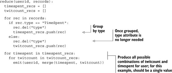
The reduce task groups records of identical type and produces all possible combinations of the two types as k3. For this specific example, you know there will be only one record of each type, so you can simplify the logic. You also can fold in the work of producing the ratio you want to calculate:

reduce(userid, records):
  for rec in records:
    rec.del("type")
  merge(records)
  emit(userid, ratio(rec["TimeSpent"], rec["TwitCount"]))

This new and improved reduce task produces the new, joined dataset:

UserID    ratio

Yvonn66   30s:48
Mario23    2s:56
Rober4     6s:2
Masan46   35s:47

There you have it: the reduce-side join in its most basic glory. One big problem with the reduce-side join is that it requires all [k2,v2] tuples to be shuffled and sorted. For our toy example, that’s no big deal. But if the datasets are very, very large, with millions of pairs per value of k2, the overhead of that step can be huge.

Reduce-side joins require shuffling and sorting data between map and reduce tasks. This incurs I/O costs, specifically network, which happens to be the slowest aspect of any distributed system. Minimizing this network I/O will improve join performance. This is where the map-side join can help.

Map-Side Join

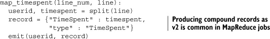
The map-side join is a technique that isn’t as general-purpose as the reduce-side join. It assumes the map tasks can look up random values from one dataset while they iterate over the other. If you happen to want to join two datasets where at least one of them can fit in memory of the map task, the problem is solved: load the smaller dataset into a hash-table so the map tasks can access it while iterating over the other dataset. In these cases, you can skip the Shuffle and Reduce Steps entirely and emit your final output from the Map Step. Let’s go back to the same example. This time you’ll put the Users dataset into memory. The new map_timespent task looks like this:

map_timespent(line_num, line):
  users_recs = read_timespent("/path/to/users.csv")
  userid, timespent = split(line)
  record = {"TimeSpent" : timespent}
  record = merge(record, users_recs[userid])
  emit(userid, ratio(record["TimeSpent"], record["TwitCount"]))

Compared to the last version, this looks like cheating! Remember, though, you can only get away with this approach when you can fit one of the datasets entirely into memory. In this case, your join will be much faster.

There are of course implications to doing joins like this. For instance, each map task is processing a single split, which is equal to one HDFS block (typically 64–128 MB), but the join dataset that it loads into memory is 1 GB. Now, 1 GB can certainly fit in memory, but the cost involved in creating a hash-table for a 1 GB dataset for every 128 MB of data being joined makes it not such a good idea.

Map-Side Join with HBase

Where does HBase come in? We originally described HBase as a giant hash-table, remember? Look again at the map-side join implementation. Replace users_recs with the Users table in TwitBase. Now you can join over the massive Users table and massive TimeSpent data set in record time! The map-side join using HBase looks like this:

map_timespent(line_num, line):
  users_table = HBase.connect("Users")
  userid, timespent = split(line)
  record = {"TimeSpent" : timespent}
  record = merge(record, users_table.get(userid, "info:twitcount"))
  emit(userid, ratio(record["TimeSpent"], record["info:twitcount"]))

Think of this as an external hash-table that each map task has access to. You don’t need to create that hash-table object for every task. You also avoid all the network I/O involved in the Shuffle Step necessary for a reduce-side join. Conceptually, this looks like figure 3.14.

Figure 3.14. Using HBase as a lookup store for the map tasks to do a map-side join

There’s a lot more to distributed joins than we’ve covered in this section. They’re so common that Hadoop ships with a contrib JAR called hadoop-datajoin to make things easier. You should now have enough context to make good use of it and also take advantage of HBase for other MapReduce optimizations.

3.5. Putting it all together

Now you see the full power of Hadoop MapReduce. The JobTracker distributes work across all the TaskTrackers in the cluster according to optimal resource utilization. If any of those nodes fails, another machine is staged and ready to pick up the computation and ensure job success.

 

 

This section provides a complete example of consuming HBase from a MapReduce application. Please keep in mind that running MapReduce jobs on an HBase cluster creates a significant burden on the cluster. You don’t want to run MapReduce jobs on the same cluster that serves your low-latency queries, at least not when you expect to maintain OLTP-style service-level agreements (SLAs)! Your online access will suffer while the MapReduce jobs run. As food for thought, consider this: don’t even run a JobTracker or TaskTrackers on your HBase cluster. Unless you absolutely must, leave the resources consumed by those processes for HBase.

3.5.1. Writing a MapReduce application

HBase is running on top of Hadoop, specifically the HDFS. Data in HBase is partitioned and replicated like any other data in the HDFS. That means running a MapReduce program over data stored in HBase has all the same advantages as a regular MapReduce program. This is why your MapReduce calculation can execute the same HBase scan as the multithreaded example and attain far greater throughput. In the MapReduce application, the scan is executing simultaneously on multiple nodes. This removes the bottleneck of all data moving through a single machine. If you’re running MapReduce on the same cluster that’s running HBase, it’s also taking advantage of any collocation that might be available. Putting it all together, the Shakespearean counting example looks like the following listing.

Listing 3.1. A Shakespearean twit counter

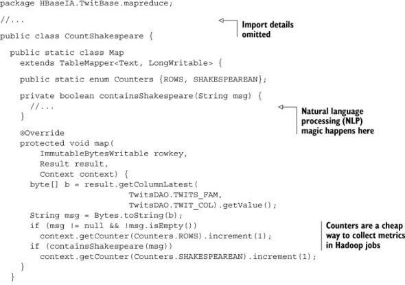
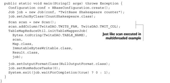
CountShakespeare is pretty simple; it packages a Mapper implementation and a main method. It also takes advantage of the HBase-specific MapReduce helper class TableMapper and the TableMapReduceUtil utility class that we talked about earlier in the chapter. Also notice the lack of a reducer. This example doesn’t need to perform additional computation in the reduce phase. Instead, map output is collected via job counters.

3.5.2. Running a MapReduce application

Would you like to see what it looks like to run a MapReduce job? We thought so. Start by populating TwitBase with a little data. These two commands load 100 users and then load 100 twits for each of those users:

$ java -cp target/twitbase-1.0.0.jar 
  HBaseIA.TwitBase.LoadUsers 100
$ java -cp target/twitbase-1.0.0.jar 
  HBaseIA.TwitBase.LoadTwits 100

Now that you have some data, you can run the CountShakespeare application over it:

$ java -cp target/twitbase-1.0.0.jar 
  HBaseIA.TwitBase.mapreduce.CountShakespeare
...
19:56:42 INFO mapred.JobClient: Running job: job_local_0001
19:56:43 INFO mapred.JobClient:  map 0% reduce 0%
...
19:56:46 INFO mapred.JobClient:  map 100% reduce 0%
19:56:46 INFO mapred.JobClient: Job complete: job_local_0001
19:56:46 INFO mapred.JobClient: Counters: 11
19:56:46 INFO mapred.JobClient: CountShakespeare$Map$Counters
19:56:46 INFO mapred.JobClient:     ROWS=9695
19:56:46 INFO mapred.JobClient:     SHAKESPEAREAN=4743
...

According to our proprietary algorithm for Shakespearean reference analysis, just under 50% of the data alludes to Shakespeare!

Counters are fun and all, but what about writing back to HBase? We’ve developed a similar algorithm specifically for detecting references to Hamlet. The mapper is similar to the Shakespearean example, except that its [k2,v2] output types are [ImmutableBytesWritable,Put]—basically, HBase rowkey and an instance of the Put command you learned in the previous chapter. Here’s the reducer code:

  public static class Reduce
    extends TableReducer<
            ImmutableBytesWritable,
            Put,
            ImmutableBytesWritable> {

    @Override
    protected void reduce(
        ImmutableBytesWritable rowkey,
        Iterable<Put> values,
        Context context) {
      Iterator<Put> i = values.iterator();
      if (i.hasNext()) {
        context.write(rowkey, i.next());
      }
    }
  }

There’s not much to it. The reducer implementation accepts [k2,{v2}], the rowkey and a list of Puts as input. In this case, each Put is setting the info:hamlet_tag column to true. A Put need only be executed once for each user, so only the first is emitted to the output context object. [k3,v3] tuples produced are also of type [ImmutableBytesWritable,Put]. You let the Hadoop machinery handle execution of the Puts to keep the reduce implementation idempotent.

3.6. Availability and reliability at scale

You’ll often hear the terms scalable, available, and reliable in the context of distributed systems. In our opinion, these aren’t absolute, definite qualities of any system, but a set of parameters that can have varied values. In other words, different systems scale to different sizes and are available and reliable in certain scenarios but not others. These properties are a function of the architectural choices that the systems make. This takes us into the domain of the CAP theorem,^[2] which always makes for an interesting discussion and a fascinating read.^[3] Different people have their own views about it,^[4] and we’d prefer not to go into a lot of detail and get academic about what the CAP theorem means for various database systems. Let’s instead jump into understanding what availability and reliability mean in the context of HBase and how it achieves them. These properties are useful to understand from the point of view of building your application so that you as an application developer can understand what you can expect from HBase as a back-end data store and how that affects your SLAs.

² CAP theorem: http://en.wikipedia.org/wiki/CAP_theorem.

³ Read more on the CAP theorem in Henry Robinson’s “CAP Confusion: Problems with ‘partition tolerance,’” Cloudera, http://mng.bz/4673.

⁴ Learn how the CAP theorem is incomplete in Daniel Abadi’s “Problems with CAP, and Yahoo’s little known NoSQL system,” DBMS Musings, http://mng.bz/j01r.

Availability

Availability in the context of HBase can be defined as the ability of the system to handle failures. The most common failures cause one or more nodes in the HBase cluster to fall off the cluster and stop serving requests. This could be because of hardware on the node failing or the software acting up for some reason. Any such failure can be considered a network partition between that node and the rest of the cluster.

When a RegionServer becomes unreachable for some reason, the data it was serving needs to instead be served by some other RegionServer. HBase can do that and keep its availability high. But if there is a network partition and the HBase masters are separated from the cluster or the ZooKeepers are separated from the cluster, the slaves can’t do much on their own. This goes back to what we said earlier: availability is best defined by the kind of failures a system can handle and the kind it can’t. It isn’t a binary property, but instead one with various degrees.

Higher availability can be achieved through defensive deployment schemes. For instance, if you have multiple masters, keep them in different racks. Deployment is covered in detail in chapter 10.

Reliability and Durability

Reliability is a general term used in the context of a database system and can be thought of as a combination of data durability and performance guarantees in most cases. For the purpose of this section, let’s examine the data durability aspect of HBase. Data durability, as you can imagine, is important when you’re building applications atop a database. /dev/null has the fastest write performance, but you can’t do much with the data once you’ve written it to /dev/null. HBase, on the other hand, has certain guarantees in terms of data durability by virtue of the system architecture.

3.6.1. HDFS as the underlying storage

HBase assumes two properties of the underlying storage that help it achieve the availability and reliability it offers to its clients.

Single Namespace

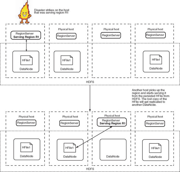
HBase stores its data on a single file system. It assumes all the RegionServers have access to that file system across the entire cluster. The file system exposes a single namespace to all the RegionServers in the cluster. The data visible to and written by one RegionServer is available to all other RegionServers. This allows HBase to make availability guarantees. If a RegionServer goes down, any other RegionServer can read the data from the underlying file system and start serving the regions that the first RegionServer was serving (figure 3.15).

Figure 3.15. If a RegionServer fails for some reason (such as a Java process dying or the entire physical node catching fire), a different RegionServer picks up the regions the first one was serving and begins serving them. This is enabled by the fact that HDFS provides a single namespace to all the RegionServers, and any of them can access the persisted files from any other.

At this point, you may be thinking that you could have a network-attached storage (NAS) that was mounted on all the servers and store the data on that. That’s theoretically doable, but there are implications to every design and implementation choice. Having a NAS that all the servers read/write to means your disk I/O will be bottlenecked by the interlink between the cluster and the NAS. You can have fat interlinks, but they will still limit the amount you can scale to. HBase made a design choice to use distributed file systems instead and was built tightly coupled with HDFS. HDFS provides HBase with a single namespace, and the DataNodes and RegionServers are collocated in most clusters. Collocating these two processes helps in that RegionServers can read and write to the local DataNode, thereby saving network I/O whenever possible. There is still network I/O, but this optimization reduces the costs.

You’re currently using a standalone HBase instance for the TwitBase application. Standalone HBase isn’t backed by HDFS. It’s writing all data onto the local file system. Chapter 9 goes into details of deploying HBase in a fully distributed manner, backed by HDFS. When you do that, you’ll configure HBase to write to HDFS in a prespecified location, which is configured by the parameter hbase.rootdir. In standalone mode, this is pointing to the default value, file:///tmp/hbase-${user.name}/hbase.

Reliability and Failure Resistance

HBase assumes that the data it persists on the underlying storage system will be accessible even in the face of failures. If a server running the RegionServer goes down, other RegionServers should be able to take up the regions that were assigned to that server and begin serving requests. The assumption is that the server going down won’t cause data loss on the underlying storage. A distributed file system like HDFS achieves this property by replicating the data and keeping multiple copies of it. At the same time, the performance of the underlying storage should not be impacted greatly by the loss of a small percentage of its member servers.

Theoretically, HBase could run on top of any file system that provides these properties. But HBase is tightly coupled with HDFS and has been during the course of its development. Apart from being able to withstand failures, HDFS provides certain write semantics that HBase uses to provide durability guarantees for every byte you write to it.

3.7. Summary

We covered quite a bit of ground this chapter, much of if at an elementary level. There’s a lot more going on in Hadoop than we can cover with a single chapter. You should now have a basic understanding of Hadoop and how HBase uses it. In practice, this relationship with Hadoop provides an HBase deployment with many advantages. Here’s an overview of what we discussed.

HBase is a database built on Hadoop. It depends on Hadoop for both data access and data reliability. Whereas HBase is an online system driven by low latency, Hadoop is an offline system optimized for throughput. These complementary concerns make for a powerful, flexible data platform for building horizontally scalable data applications.

Hadoop MapReduce is a distributed computation framework providing data access. It’s a fault-tolerant, batch-oriented computing model. MapReduce programs are written by composing map and reduce operations into Jobs. Individual tasks are assumed to be idempotent. MapReduce takes advantage of the HDFS by assigning tasks to blocks on the file system and distributing the computation to the data. This allows for highly parallel programs with minimal distribution overhead.

HBase is designed for MapReduce interaction; it provides a TableMapper and a TableReducer to ease implementation of MapReduce applications. The TableMapper allows your MapReduce application to easily read data directly out of HBase. The TableReducer makes it easy to write data back to HBase from MapReduce. It’s also possible to interact with the HBase key-value API from within the Map and Reduce Steps. This is helpful for situations where all your tasks need random access to the same data. It’s commonly used for implementing distributed map-side joins.

If you’re curious to learn more about how Hadoop works or investigate additional techniques for MapReduce, Hadoop: The Definitive Guide by Tom White (O’Reilly, 2009) and Hadoop in Action by Chuck Lam (Manning, 2010) are both great references.