
Chapter 8. Scaling GIS on HBase
In this chapter, we’ll use HBase to tackle a new domain: Geographic Information Systems (GIS). GIS is an interesting area of exploration because it poses two significant challenges: latency at scale and modeling spatial locality. We’ll use the lens of GIS to demonstrate how to adapt HBase to tackle these challenges. To do so, you’ll need to use domain-specific knowledge to your advantage.
8.1. Working with geographic data
Geographic systems are frequently used as the foundation of an online, interactive user experience. Consider a location-based service, such as Foursquare, Yelp, or Urban Spoon. These services strive to provide relevant information about hundreds of millions of locations all over the globe. Users of these applications depend on them to find, for instance, the nearest coffee shop in an unfamiliar neighborhood. They don’t want a MapReduce job standing between them and their latte. We’ve already discussed HBase as a platform for online data access, so this first constraint seems a reasonable match for HBase. Still, as you’ve seen in previous chapters, HBase can only provide low request latency when your schema is designed to use the physical storage of data. This brings you conveniently to the second challenge: spatial locality.
Spatial locality in GIS data is tricky. We’ll spend a major portion of this chapter explaining an algorithm called the geohash, which is a solution to this problem. The idea is to store data so that all the information about a place on Earth is stored close together. That way, when you want to investigate that location, you need to make as few data requests as possible. You also want the information about places that are close together on Earth to be stored close together on disk. If you’re accessing information about Midtown Manhattan, it’s likely you’ll also want information about Chelsea and Greenwich Village. You want to store that data closer to the Midtown data than, say, data about Brooklyn or Queens. By storing information about these spatially similar places so that the information is physically close together, you can potentially achieve a faster user experience.
This idea of spatial locality is similar to but not the same as Hadoop’s concept of data locality. In both cases, we’re considering the work of moving data. Spatial locality in GIS is about storing data with a similar spatial context in a similar place. Data locality in Hadoop is about performing the data access and computation on the machine in the cluster where that data is physically stored. Both cases are about minimizing the overhead of working with the data, but that’s where the similarity ends.
The simplest form of geographic data, a single point on Earth, is composed of two equally relevant dimensions: longitude (X-axis) and latitude (Y-axis). Even this is a simplification. Many professional GIS systems must also consider a Z-axis, such as elevation or altitude, in addition to the X- and Y-axes. Many GIS applications also track position over time, which presents all the challenges of time-series data discussed in the previous chapter. Both kinds of data locality are critical when designing systems providing low-latency data access. HBase makes this clear through schema design and use of the rowkey. The sorted rowkey gives you direct control over the locality of storage of your data.
How do you guarantee data locality for your spatial data when both dimensions (or perhaps all four dimensions) are equally relevant? Building an index exclusively over longitude, for example, places New York City closer to Chicago than Seattle. But as figure 8.1 illustrates, it would also give you Bogotá, Columbia, before the District of Columbia. Considering only one dimension isn’t sufficient for the needs of GIS.
Figure 8.1. In GIS, all dimensions matter. Building an index of the world’s cities over only longitude, the X-axis, would order data inaccurately for a certain set of queries.

Note
This chapter explores spatial concepts that can be communicated effectively only via illustrations. Toward that end, we’ve employed a browser-based cartography library called Leaflet to build these illustrations with repeatable precision. GitHub claims this chapter’s project is 95% JavaScript. The map tiles behind the figures are of the beautiful Watercolor tile set from Stamen Design and are built from completely open data. Learn more about Leaflet at http://leaflet.cloudmade.com. Watercolor lives at http://maps.stamen.com/#watercolor. The underlying data is from OpenStreetMap, a project like Wikipedia, but for geographic data. Find out more at www.openstreetmap.org.
How do you organize your data such that New York City (NYC) and Washington, D.C., are closer than NYC and Bogotá? You’ll tackle this challenge over the course of this chapter in the form of a specialized spatial index. You’ll use this index as the foundation of two kinds of spatial queries. The first query, “k nearest neighbors,” is built directly on that index. The second query, “polygon within,” is implemented twice. The first time, it’s built against the spatial index alone. The second implementation moves as much work as possible to the server side, in the form of a custom filter. This will maximize the work performed in your HBase cluster and minimize the superfluous data returned to the client. Along the way, you’ll learn enough of this new domain to turn HBase into a fully capable GIS machine. The devil, as they say, is in the details, so let’s zoom in from this question of distance between international cities and solve a much more local problem.
The code and data used through the course of this chapter are available on our GitHub account. This project can be found at https://github.com/hbaseinaction/gis.
8.2. Designing a spatial index
Let’s say you’re visiting NYC and need an internet connection. “Where’s the nearest wifi hotspot?” How might an HBase application help you answer that question? What kind of design decisions go into solving that problem, and how can it be solved in a scalable way?
You know you want fast access to a relevant subset of the data. To achieve that, let’s start with two simple and related goals:
| You want to store location points on disk such that points close to each other in space are close to each other on disk. | |
| You want to retrieve as few points as possible when responding to a query. |
Achieving these goals will allow you to build a highly responsive online application against a spatial dataset. The main tool HBase gives you for tackling both of these goals is the rowkey. You saw in previous chapters how to index multiple attributes in a compound rowkey. Based on the D.C. versus Bogotá example, we have a hunch it won’t meet the first design goal. It doesn’t hurt to try, especially if you can learn something along the way. It’s easy to implement, so let’s evaluate the basic compound rowkey before trying anything more elaborate.
Let’s start by looking at the data. New York City has an open-data program and publishes many datasets.[1] One of those datasets[2] is a listing of all the city’s wifi hotspots. We don’t expect you to be familiar with GIS or GIS data, so we’ve preprocessed it a bit. Here’s a sample of that data:
1 Some of those datasets are pretty cool, in particular the Street Tree Census data. Look for yourself at https://nycopendata.socrata.com/.
2 The raw dataset used in this chapter is available at https://nycopendata.socrata.com/d/ehc4-fktp
        X             Y       ID   NAME
1  -73.96974759  40.75890919  441  Fedex Kinko's
2  -73.96993203  40.75815170  442  Fedex Kinko's
3  -73.96873588  40.76107453  463  Smilers 707
4  -73.96880474  40.76048717  472  Juan Valdez NYC
5  -73.96974993  40.76170883  219  Startegy Atrium and Cafe
6  -73.96978387  40.75850573  388  Barnes & Noble
7  -73.96746533  40.76089302  525  McDonalds
8  -73.96910155  40.75873061  564  Public Telephone
9  -73.97000655  40.76098703  593  Starbucks
You’ve processed the data into a tab-separated text file. The first line contains the column names. The columns X and Y are the longitude and latitude values, respectively. Each record has an ID, a NAME, and a number of other columns.
A great thing about GIS data is that it lends itself nicely to pictures! Unlike other kinds of data, no aggregations are required to build a meaningful visualization—just throw points on a map and see what you have. This sample data looks like figure 8.2.
Figure 8.2. Find the wifi. Geographic data wants to be seen, so draw it on a map. Here’s a sampling of the full dataset—a handful of places to find a wifi connection in Midtown Manhattan.

Based on the goals outlined earlier, you now have a pretty good spot-check for your schema designs. Remember goal ![]() . Point 388 is close to point 441 on the map, so those records should be close to each other in the database. As goal
. Point 388 is close to point 441 on the map, so those records should be close to each other in the database. As goal ![]() states, if you want to retrieve those two points, you shouldn’t have to retrieve point 219 as well.
states, if you want to retrieve those two points, you shouldn’t have to retrieve point 219 as well.
Now you know the goals and you know the data. It’s time to take a stab at the schema. As you learned in chapter 4, design of the rowkey is the single most important thing you can do in your HBase schema, so let’s start there.
8.2.1. Starting with a compound rowkey
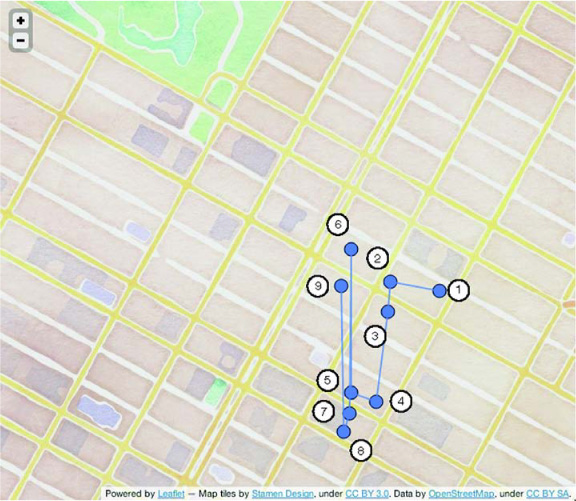
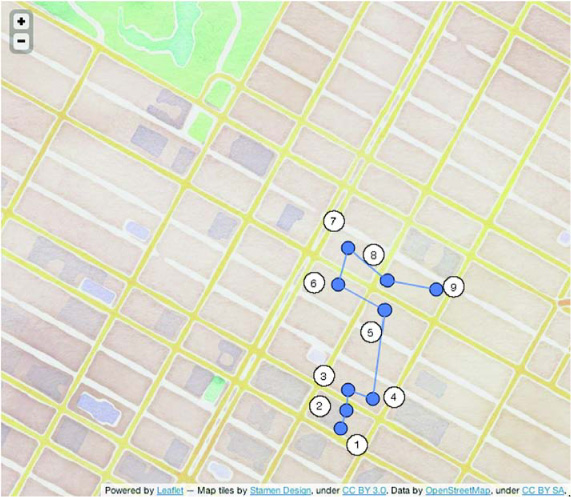
We claimed earlier that concatenating X- and Y-axis values as the rowkey won’t cut it for an efficient schema. We cited the D.C. versus Bogotá example as proof. Let’s see why. Sort the sample records first by longitude, then latitude, and connect the dots. Figure 8.3 does just that. When you store data this way, scanning returns results ordered from 1 to 9. Notice in particular the distance between steps 6 and 7, and steps 8 and 9. This sorting results in lots of hopping between the northern and southern clusters because of sorting first on longitude, then latitude.
Figure 8.3. A naïve approach to spatial schema design: concatenated axes values. This schema fails the first objective of mapping spatial locality to record locality.
This schema design does okay with goal ![]() , but that’s likely because the data sample is small. Goal
, but that’s likely because the data sample is small. Goal ![]() is also poorly represented. Every jump from the northern cluster to the southern cluster represents retrieval of data you
don’t need. Remember the Bogotá versus D.C. example from figure 8.1? That’s precisely the problem you see in this schema design. Points close to each other aren’t necessarily close together
as records in HBase. When you translate this to a rowkey scan, you have to retrieve every possible point along the latitude
for the desired longitude range. Of course, you could work around this flaw in the design. Perhaps you could build a latitude
filter, implemented as a RegexStringComparator attached to a RowFilter. At least that way you could keep all that extra data from hitting the client. That’s not ideal, though. A filter is reading
records out of the store in order to execute the filter logic. It would be better to never touch that data, if you can avoid
it.
is also poorly represented. Every jump from the northern cluster to the southern cluster represents retrieval of data you
don’t need. Remember the Bogotá versus D.C. example from figure 8.1? That’s precisely the problem you see in this schema design. Points close to each other aren’t necessarily close together
as records in HBase. When you translate this to a rowkey scan, you have to retrieve every possible point along the latitude
for the desired longitude range. Of course, you could work around this flaw in the design. Perhaps you could build a latitude
filter, implemented as a RegexStringComparator attached to a RowFilter. At least that way you could keep all that extra data from hitting the client. That’s not ideal, though. A filter is reading
records out of the store in order to execute the filter logic. It would be better to never touch that data, if you can avoid
it.
This schema design, placing one dimension ahead of the other in the rowkey, also implies an ordered relationship between dimensions that doesn’t exist. You can do better. To do so, you need to learn about a trick the GIS community devised for solving these kinds of problems: the geohash.
8.2.2. Introducing the geohash
As the previous example shows, longitude and latitude are equally important in defining the location of a point. In order to use them as the basis for the spatial index, you need an algorithm to combine them. Such an algorithm will create a value based on the two dimensions. That way, two values produced by the algorithm are related to each other in a way that considers both dimensions equally. The geohash does exactly this.
A geohash is a function that turns some number of values into a single value. For it to work, each of those values must be from a dimension with a fixed domain. In this case, you want to turn both longitude and latitude into a single value. The longitude dimension is bounded by the range [-180.0, 180.0], and the latitude dimension is bounded by the range [-90.0, 90.0]. There are a number of ways to reduce multiple dimensions to a single one, but we’re using the geohash here because its output preserves spatial locality.
A geohash isn’t a flawless encoding of the input data. For you audiophiles, it’s a bit like an MP3 of your source recording. The input data is mostly there, but only mostly. Like an MP3, you must specify a precision when calculating a geohash. You’ll use 12 geohash characters for the precision because that’s the highest precision you can fit in an 8-byte Long and still represent a meaningful character string. By truncating characters from the end of the hash, you get a less precise geohash and a correspondingly less precise selection of the map. Where full precision represents a point, partial precision gives you an area on the map, effectively a bounding box around an area in space. Figure 8.4 illustrates the decreasing precision of a truncated geohash.
Figure 8.4. Truncating a geohash. By dropping characters from the end of a geohash, you drop precision from the space that hash represents. A single character goes a long way.
For a given geohash prefix, all points within that space match the common prefix. If you can fit your query inside a geohash
prefix’s bounding box, all matching points will share a common prefix. That means you can use HBase’s prefix scan on the rowkeys
to get back a set of points that are all relevant to the query. That accomplishes goal ![]() . But as figure 8.4 illustrates, if you have to choose an overly generous precision, you’ll end up with much more data than you need. That violates
goal
. But as figure 8.4 illustrates, if you have to choose an overly generous precision, you’ll end up with much more data than you need. That violates
goal ![]() . You need to work around these edge cases, but we’ll cover that a little later. For now, let’s look at some real points.
. You need to work around these edge cases, but we’ll cover that a little later. For now, let’s look at some real points.
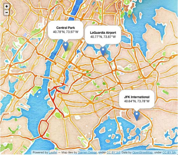
Consider these three locations: LaGuardia Airport (40.77° N, 73.87° W), JFK International Airport (40.64° N, 73.78° W), and Central Park (40.78° N, 73.97° W). Their coordinates geohash to the values dr5rzjcw2nze, dr5x1n711mhd, and dr5ruzb8wnfr, respectively. You can look at those points on the map in figure 8.5 and see that Central Park is closer to LaGuardia than JFK. In absolute terms, Central Park to LaGuardia is about 5 miles, whereas Central Park to JFK is about 14 miles.
Figure 8.5. Relative distances. When viewed on a map, it’s easy to see that the distance between Central Park and JFK is much farther than the distance between Central Park and LaGuardia. This is precisely the relationship you want to reproduce with your hashing algorithm.
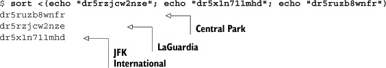
Because they’re closer to each other spatially, you expect Central Park and LaGuardia to share more common prefix characters than Central Park and JFK. Sure enough:
Now that you understand how a geohash can work for you, we’ll show you how to calculate one. Don’t worry; you won’t be hashing all these points by hand. With HBase, it’s useful to understand how it works in order to use it effectively. Likewise with the geohash, understanding how it’s constructed will help you understand its edge cases.
8.2.3. Understand the geohash
The geohashes you’ve seen are all represented as character strings in the Base32 encoding alphabet.[3] In reality, the geohash is a sequence of bits representing an increasingly precise subdivision of longitude and latitude.
3 Base32 is an encoding used to represent a binary value as a sequence of ASCII characters. Note that although geohash uses an alphabet of characters similar to that of Base32, the geohash spec doesn’t follow the Base32 RFC. Learn more about Base32 at http://en.wikipedia.org/wiki/Base32.
For instance, 40.78° N is a latitude. It falls in the upper half[4] of the range [-90.0, 90.0], so its first geohash bit is 1. Its second bit is 0 because 40.78 is in the lower half of the range [0.0, 90.0]. The third range is [0.0, 45.0], and 40.78 falls in the upper half, so the third bit is 1.
4 When including a direction, degrees of latitude are measured from 0.0 to 90.0 with the northern hemisphere corresponding to positive values and the southern hemisphere to negative values on the absolute latitude range. Likewise, degrees of longitude are measured from 0.0 to 180.0 with the eastern hemisphere indicating positive values and western hemisphere indicating negative values.
The contribution provided by each dimension is calculated by halving the value range and determining which half the point resides in. If the point is greater than or equal to the midpoint, it’s a 1-bit. Otherwise, it’s a 0-bit. This process is repeated, again cutting the range in half and selecting a 1 or 0 based on where the target point lies. This binary partitioning is performed on both the longitude and latitude values. Rather than using the bit sequence from each dimension independently, the encoding weaves the bits together to create the hash. The spatial partitioning is why geohashes have the spatial locality property. The weaving of bits from each dimension is what allows for the prefix-match precision trickery.
Now that you understand how each component is encoded, let’s calculate a full value. This process of bisecting the range and selecting a bit is repeated until the desired precision is achieved. A bit sequence is calculated for both longitude and latitude, and the bits are interwoven, longitude first, then latitude, out to the target precision. Figure 8.6 illustrates the process. Once the bit sequence is calculated, it’s encoded to produce the final hash value.
Figure 8.6. Constructing a geohash. The first 3 bits from longitude and latitude are calculated and woven to produce a geohash of 6-bit precision. The example data we discussed previously executed this algorithm out to 7 Base32 characters, or 35-bit precision.

Now that you understand why the geohash is useful to you and how it works, let’s plug it in for your rowkey.
8.2.4. Using the geohash as a spatially aware rowkey
The geohash makes a great choice for the rowkey because it’s inexpensive to calculate and the prefix gets you a long way toward finding nearest neighbors. Let’s apply it to the sample data, sort by geohash, and see how you’re doing on prefixes. We’ve calculated the geohash for each point using a library[5] and added it to the data. All of the data in the sample is relatively close together, so you expect a good deal of prefix overlap across the points:
5 We’re using Silvio Heuberger’s Java implementation at https://github.com/kungfoo/geohash-java. We’ve made it available in Maven for easy distribution.
      GEOHASH         X             Y        ID  NAME
1  dr5rugb9rwjj  -73.96993203  40.75815170  442  Fedex Kinko's
2  dr5rugbge05m  -73.96978387  40.75850573  388  Barnes & Noble
3  dr5rugbvggqe  -73.96974759  40.75890919  441  Fedex Kinko's
4  dr5rugckg406  -73.96910155  40.75873061  564  Public Telephone
5  dr5ruu1x1ct8  -73.96880474  40.76048717  472  Juan Valdez NYC
6  dr5ruu29vytq  -73.97000655  40.76098703  593  Starbucks
7  dr5ruu2y5vkb  -73.96974993  40.76170883  219  Startegy Atrium and Cafe
8  dr5ruu3d7x0b  -73.96873588  40.76107453  463  Smilers 707
9  dr5ruu693jhm  -73.96746533  40.76089302  525  McDonalds
Sure enough, you get five characters of common prefix. That’s not bad at all! This means you’re a long way toward the distance
query and goal ![]() with a simple range scan. For context, figure 8.7 puts this data on a map.
with a simple range scan. For context, figure 8.7 puts this data on a map.
Figure 8.7. Seeing prefix matches in action. If the target search is in this area, a simple rowkey scan will get the data you need. Not only that, but the order of results makes a lot more sense than the order in figure 8.3.
This is much better than the compound rowkey approach, but it’s by no means perfect. All these points are close together,
within a couple blocks of each other. Why are you only matching on 5 of 12 characters? We would hope data this spatially close
would be stored much closer together. Thinking back to figure 8.4, the difference in size of the spatial area covered by a prefix scan of five versus six versus seven characters is significant—far
more than a couple of blocks. You’d make strides toward goal ![]() if you could make two scans of prefix six rather than a single scan of prefix five. Or better still, how about five or six
scans of prefix seven? Let’s look at figure 8.8, this time with more perspective. The geohash boxes for both the six-character and seven-character geohash prefixes are overlaid.
if you could make two scans of prefix six rather than a single scan of prefix five. Or better still, how about five or six
scans of prefix seven? Let’s look at figure 8.8, this time with more perspective. The geohash boxes for both the six-character and seven-character geohash prefixes are overlaid.
Figure 8.8. Prefix matches with geohash overlay. Lots of additional, unnecessary area is introduced into the query result by using the 6-character prefix. An ideal implementation would use only 7-character prefixes to minimize the amount of extra data transmitted over the wire.
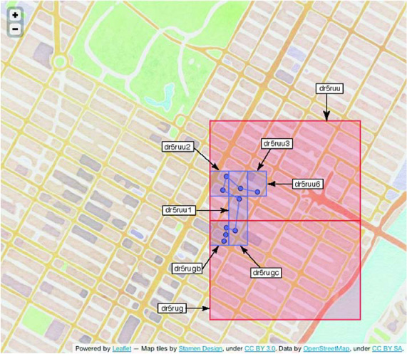
Compared to the target query area, the six-character prefix match areas are huge. Worse still, the query spans two of those larger prefixes. Seen in this context, those five characters of common prefix include far more data than you need. Relying on prefix match results in scanning a huge amount of extra area. Of course, there’s a trade-off. If your data isn’t dense at this precision level, executing fewer, longer scans isn’t such a big deal. The scans don’t return too much superfluous data, and you can minimize the remote procedure call (RPC) overhead. If your data is dense, running more, shorter scans will reduce the number of excess points transported over the wire. Plus, if there’s one thing that computers are getting good at these days, it’s parallelism. Execute each of those shorter scans on its own CPU core, and the query is still as fast as the slowest scan.
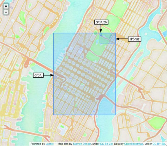
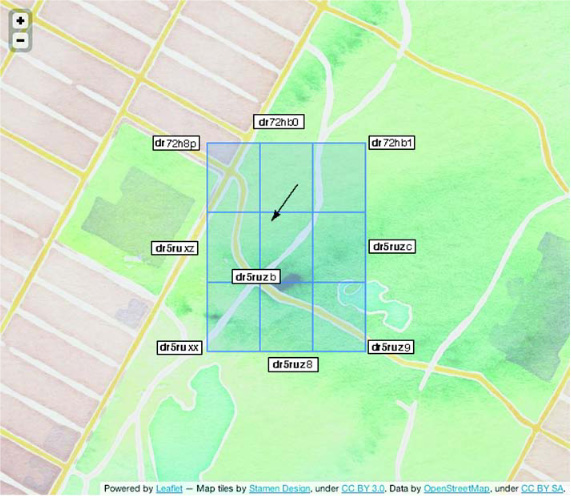
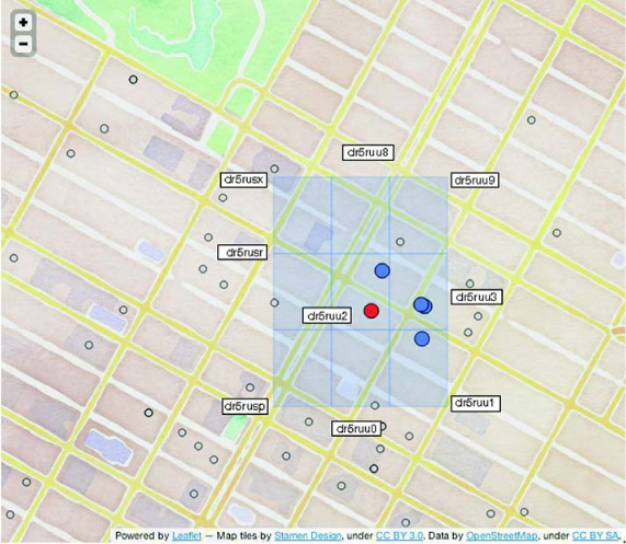
Let’s scroll the map over to a different part of Manhattan, not far from the space we’ve explored thus far. Look at figure 8.9. Notice that the geohash of the center box has six characters (dr5ruz) of prefix in common with the boxes to its east, southeast, and south. But there are only five characters (dr5ru) in common with the west and southwest boxes. If five characters of common prefix is bad, then the prefix match with the entire northern row is abysmal, with only two characters (dr) in common! This doesn’t happen every time, but it does happen with a surprisingly high frequency. As a counterexample, all eight neighbors of the southeast box (dr5ruz9) share a common six-character prefix.
Figure 8.9. Visualizing the geohash edge case. The encoding isn’t perfect; this is one such case. Imagine a nearest-neighbor search falling on the point under the arrow in this illustration. It’s possible you’ll find a neighbor in a tile with only two characters of common prefix.
The geohash is effective, but you can’t use a simple naïve prefix match either. Based on these figures, it looks like the optimal approach for the data is to scan the center tile and its eight neighbors. This approach will guarantee correct results while minimizing the amount of unnecessary network IO. Luckily, calculating those neighbors is a simple bit-manipulation away. Explaining the details of that manipulation is beyond the scope of our interest, so we’ll trust the geohash library to provide that feature.
The geohash is approximating the data space. That is, it’s a function that computes a value on a single output dimension based on input from multiple dimensions. In this case, the dimensionality of the input is only 2, but you can imagine how this could work for more. This is a form of linearization, and it’s not the only one. Other techniques such as the Z-order curve[6] and the Hilbert curve[7] are also common. These are both classes of space-filling curves:[8] curves defined by a single, uninterrupted line that touches all partitions of a space. None of these techniques can perfectly model a two-dimensional plane on a one-dimensional line and maintain the relative characteristics of objects in those spaces. We choose the geohash because, for our purposes, its error cases are less bad than the others.
6 The Z-order curve is extremely similar to the geohash, involving the interleaving of bits. Read more at http://en.wikipedia.org/wiki/Z-order_curve.
7 The Hilbert curve is similar to a Z-order curve. Learn more at http://en.wikipedia.org/wiki/Hilbert_curve.
8 Read more about space-filling curves at http://en.wikipedia.org/wiki/Space-filling_curves.
8.3. Implementing the nearest-neighbors query
Now it’s time to put your newfound geohash knowledge into practice by implementing the query. Remember the question you’re trying to answer: “Where are the five nearest wifi hotspots?” That sounds like a function with three arguments: a target location, in the form of a latitude and longitude, and the maximum number of results, something along the lines of the following:
public Collection<QueryMatch> queryKNN(double lat, double lon, int n) {
  ...
}
QueryMatch is a data class you’ll use to keep track of, well, a query result. Here are the steps involved:
- Construct the target GeoHash.
- Iterate through it and its eight neighbors to find candidate results. The results from each scan are ranked according to distance from the target point and limited to only the n closest results.
- Rank and limit the results of the nine scans to compute the final n results returned to the caller.
You’ll implement this in two functions: one to handle the HBase scan and the other to handle the geohash and aggregation. In pseudo-code, the first function looks like this:
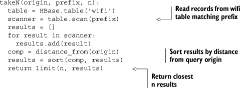
There’s nothing particularly special here; you’re interacting with HBase as you’ve done before. You don’t need to hang onto all the query results from each scan, only the closest n. That cuts down on the memory usage of the query process, especially if you’re forced to use a shorter prefix than desired.
The main query function builds on the takeN helper function. Again, here it is in pseudo-code:
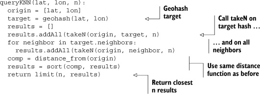
The queryKNN function handles generating the geohash from the query target, calculating the nine prefixes to scan, and consolidating the results. As you saw in figure 8.9, all nine prefixes must be scanned to guarantee correct results. The same technique used to limit memory usage in takeN is used to pare down the final results. This is also where you’d want to put any concurrency code, if you’re so inclined.
Now let’s translate the pseudo-code into the Java implementation. Google’s Guava[9] library provides a handy class to manage the sorted, size-limited bucket of results via the MinMaxPriorityQueue. It accepts a custom Comparator for order maintenance and enforcing the eviction policy; you’ll need to build one for your QueryMatch class. The Comparator is based on distance from the origin of the query target. The java.awt.geom.Point2D class gives you a simple distance function that’s good enough[10] for your needs. Let’s start with the helpers, QueryMatch and DistanceComparator:
9 Guava is the missing utils library for Java. If you’re a professional Java developer and you’ve never explored it, you’re missing out. There’s a nice overview on the wiki: http://mng.bz/ApbT.
10 We’re being pretty flippant with the domain specifics here. Realistically, you don’t want to use a simple distance function, especially if you’re calculating distances spanning a large area. Remember, the Earth is roundish, not flat. Simple things like Euclidean geometry need not apply. In general, take extra care when calculating nonrelative values, especially when you want to think in uniform geometries like circles and squares or return human-meaningful units like miles or kilometers.
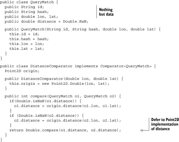
Normally you wouldn’t write Comparators the way we did in the code example. Don’t do this in your normal code! We’ve done so here to make it easier to inspect the results from within the text. It’s only to help explain what’s happening here. Really, please, don’t do this!
With the result sorting in place, you need a Java version of takeN, the method to perform the HBase scan. Each prefix needs to sort and limit the set of partial results returned, so it takes a Comparator in addition to the prefix and n. That’s instead of receiving the origin point as you did in pseudo-code:
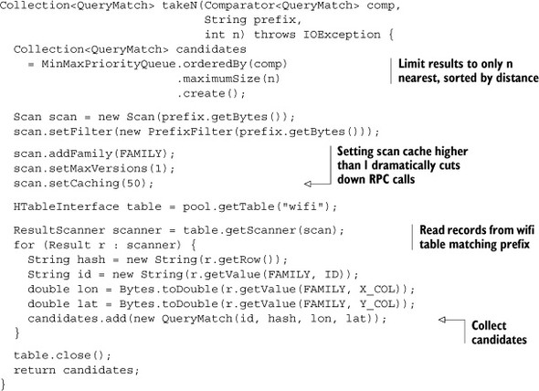
This is the same kind of table scan used when you learned about scans in chapter 2. The only new thing to point out here is the call to Scan.setCaching(). That method call sets the number of records returned per RPC call the scanner makes to 50—a somewhat arbitrary number, based on the number of records traversed by the scan and the size of each record. For this dataset, the records are small and the idea is to restrict the number of records scanned via the geohash. Fifty should be far more data than you expect to pull from a single scan at this precision. You’ll want to play with that number to determine an optimal setting for your use case. There’s a useful post[11] on the hbase-user[12] mailing list describing in detail the kinds of trade-offs you’re balancing with this setting. Be sure to play with it, because anything is likely better than the default of 1.
12 You mean you’ve not subscribed to hbase-user yet? Get on it! Subscribe and browse the archives from http://mail-archives.apache.org/mod_mbox/hbase-user/.
Finally, fill out the stub you defined earlier. It computes a GeoHash from the target query point and calls takeN over that prefix as well as the eight surrounding neighbors. Results are aggregated using the same limiting MinMaxPriorityQueue class used in takeN:
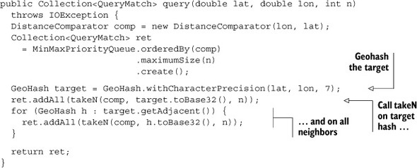
Instantiating a Comparator is simple, instantiating the queue is simple, and the for loop over the geohash neighbors is simple. The only odd thing here is the construction of the GeoHash. This library allows you to specify a character precision. Earlier in the chapter, you wanted to hash a point in space, so you used the maximum precision you could get: 12 characters. Here the situation is different. You’re not after a single point, but a bounding box. Choose a precision that’s too high, and you won’t query over enough space to find n matches, particularly when n is small. Choose a precision that’s too low, and your scans will traverse orders of magnitude more data than you need. Using seven characters of precision makes sense for this dataset and this query. Different data or different values of n will require a different precision. Striking that balance can be tricky, so our best advice is to profile your queries and experiment. If all the queries look roughly the same, perhaps you can decide on a value. Otherwise, you’ll want to build a heuristic to decide on a precision based on the query parameters. In either case, you need to get to know your data and your application!
Notice that we said to choose your geohash prefix precision based on the application-level query. You always want to design your HBase scans according to the query instead of designing them based on the data. Your data will change over time, long after your application is “finished.” If you tie your queries to the data, your query performance will change along with the data. That means a fast query today may become a slow query tomorrow. Building scans based on the application-level query means a “fast query” will always be fast relative to a “slow query.” If you couple the scans to the application-level query, users of your application will enjoy a more consistent experience.
Toss together a simple main(), and then you can see if it all works. Well, almost. You need to load the data too. The details of parsing a tab-separated values (TSV) file aren’t terribly interesting. The part you care about is using the GeoHash library to construct the hash you use for a rowkey. That code is simple enough. These are points, so you use 12 characters of precision. Again, that’s the longest printable geohash you can construct and still fit in a Java long:
double lat = Double.parseDouble(row.get("lat"));
double lon = Double.parseDouble(row.get("lon"));
String rowkey = GeoHash.withCharacterPrecision(lat, lon, 12).toBase32();
Now you have everything you need. Start by opening the shell and creating a table. The column family isn’t particularly important here, so let’s choose something short:
$ echo "create 'wifi', 'a'" | hbase shell
HBase Shell; enter 'help<RETURN>' for list of supported commands.
Type "exit<RETURN>" to leave the HBase Shell
Version 0.92.1, r1298924, Fri Mar  9 16:58:34 UTC 2012

create 'wifi', 'a'
0 row(s) in 6.5610 seconds
The test data is packaged in the project, so you have everything you need. Build the application, and run the Ingest tool against the full dataset:
$ mvn clean package
...
[INFO] -----------------------------------------------------
[INFO] BUILD SUCCESS
[INFO] -----------------------------------------------------
$ java -cp target/hbaseia-gis-1.0.0.jar
  HBaseIA.GIS.Ingest
  wifi data/wifi_4326.txt
Geohashed 1250 records in 354ms.
Looks good! It’s time to run a query. For the target point, let’s cheat a little and choose the coordinates of one of the existing data points. If the distance algorithm isn’t completely broken, that point should be the first result. Let’s center the query on ID 593:
$ java -cp target/hbaseia-gis-1.0.0.jar
  HBaseIA.GIS.KNNQuery -73.97000655 40.76098703 5
Scan over 'dr5ruu2' returned 2 candidates.
Scan over 'dr5ruu8' returned 0 candidates.
Scan over 'dr5ruu9' returned 1 candidates.
Scan over 'dr5ruu3' returned 2 candidates.
Scan over 'dr5ruu1' returned 1 candidates.
Scan over 'dr5ruu0' returned 1 candidates.
Scan over 'dr5rusp' returned 0 candidates.
Scan over 'dr5rusr' returned 1 candidates.
Scan over 'dr5rusx' returned 0 candidates.
<QueryMatch:  593, dr5ruu29vytq, -73.9700, 40.7610, 0.00000 >
<QueryMatch:  219, dr5ruu2y5vkb, -73.9697, 40.7617, 0.00077 >
<QueryMatch: 1132, dr5ruu3d9tn9, -73.9688, 40.7611, 0.00120 >
<QueryMatch:  463, dr5ruu3d7x0b, -73.9687, 40.7611, 0.00127 >
<QueryMatch:  472, dr5ruu1x1ct8, -73.9688, 40.7605, 0.00130 >
Excellent! ID 593, the point that matched the query target, comes up first! We’ve added a bit of debugging information to help understand these results. The first set of output is the contributions from each of the prefix scans. The second set of output is the match results. The fields printed are ID, geohash, longitude, latitude, and distance from the query target. Figure 8.10 illustrates how the query comes together spatially.
Figure 8.10. Visualizing query results. This simple spiraling technique searches out around the query coordinate looking for matches. A smarter implementation would take into account the query coordinate’s position within the central spatial extent. Once the minimum number of matches had been found, it would skip any neighbors that are too far away to contribute.
That’s pretty cool, right? As you likely noticed, all the comparison work happened on the client side of the operation. The scans pulled down all the data, and postprocessing happened in the client. You have a cluster of machines in your HBase deployment, so let’s see if you can put them to work. Perhaps you can use some other features to extend HBase into a full-fledged distributed geographic query engine.
8.4. Pushing work server-side
The sample dataset is pretty small, only 1,200 points and not too many attributes per point. Still, your data will grow, and your users will always demand a faster experience. It’s generally a good idea to push as much work server-side as you can. As you know, HBase gives you two mechanisms for pushing work into the RegionServers: filters and coprocessors. In this section, you’ll extend the wifi example you’ve started. You’ll implement a new kind of geographic query, and you’ll do so using a custom filter. Implementing a custom filter has some operational overhead, so before you do that you’ll make an improvement on the way you use the geohash.
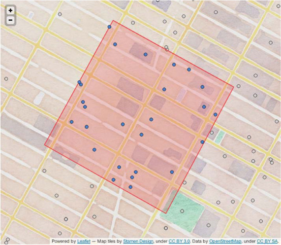
You’ll start by changing the query. Instead of looking for wifi hotspots near a particular location, let’s look for all hotspots in a requested space. Specifically, you’ll answer the query, “What are all wifi hotspots within a block of Times Square?” That space containing Times Square is a relatively simple shape to draw by hand: just four corners. You’ll use the points (40.758703° N, 73.980844° W), (40.761369° N, 73.987214° W), (40.756400° N, 73.990839° W), (40.753642° N, 73.984422° W). The query region, along with the data, is illustrated in figure 8.11. As you can see, you expect to receive about 25 points in the query results.
Figure 8.11. Querying within a block of Times Square. We used Google Earth to eyeball the four corners of the query space. It looks like all those flashy sign boards sucked up the wifi; it’s not very dense compared to other parts of the city. You can expect about 25 points to match your query.
This is a pretty simple shape, drawn by hand and overlaid on the map. What you have here is a simple polygon. There are plenty of sources for polygons you might use in your query. For instance, a service like Yelp might provide a user with predefined polygons describing local neighborhood boundaries. You could even allow the user of your application to sketch their query polygon by hand. The approach you’re going to take works as well with this simple rectangle as with a more complex shape.
With the query shape defined, it’s time to devise a plan for implementing the query. Like the k-nearest-neighbors query, you want the implementation to minimize the number of candidate points read out of HBase. You have the geohash index, which takes you fairly far along. The first step is to translate the query polygon into a set of geohash scans. As you know from the previous query, that will give you all candidate points without too many extra. The second step is to pull out only the points that are contained by the query polygon. Both of these will require help from a geometry library. Luckily, you have such a companion in the JTS Topology Suite (JTS).[13] You’ll use that library to bridge the gap between the geohash and the query polygon.
13 JTS is a full-featured library for computational geometry in Java. Check it out at http://tsusiatsoftware.net/jts/main.html.
8.4.1. Creating a geohash scan from a query polygon
For this step of query building, you need to work out exactly which prefixes you want to scan. As before, you want to minimize both the number of scans made and the spatial extent covered by the scans. The GeoHash.getAdjacent() method gave you a cheap way to extend the query area before stepping up to a less precise geohash. Let’s use that to find a suitable set of scans—a minimal bounding set of prefixes. Before we describe the algorithm, it’s helpful to know a couple of geometry tricks.
The first trick you want to use is the centroid,[14] a point at the geometric center of a polygon. The query parameter is a polygon, and every polygon has a centroid. You’ll use the centroid to start your search for a minimum bounding prefix scan. JTS can calculate this for you using the Geometry.getCentroid() method, assuming you have a Geometry instance. Thus you need a way to make Geometry an object from your query argument. There’s a simple text format for describing geometries called well-known text (WKT).[15] The query around Times Square translated into WKT looks like this:
14Centroid is a mathematical term with a strict meaning in formal geometry. One point of note is that the centroid of a polygon isn’t always contained by it. That isn’t the case with the query example; but in real life data is messy, and this does happen. The Wikipedia article provides many useful example illustrations: http://en.wikipedia.org/wiki/Centroid.
15 More examples of well-known text can be found at http://en.wikipedia.org/wiki/Well-known_text.
 POLYGON ((-73.980844 40.758703,
           -73.987214 40.761369,
           -73.990839 40.756400,
           -73.984422 40.753642,
           -73.980844 40.758703))
That’s Times Square in data. Technically speaking, a polygon is a closed shape, so the first and last point must match. The application accepts WKT as the input query. JTS provides a parser for WKT, which you can use to create a Geometry from the query input. Once you have that, the centroid is just a method call away:
String wkt = ...
WKTReader reader = new WKTReader();
Geometry query = reader.read(wkt);
Point queryCenter = query.getCentroid();
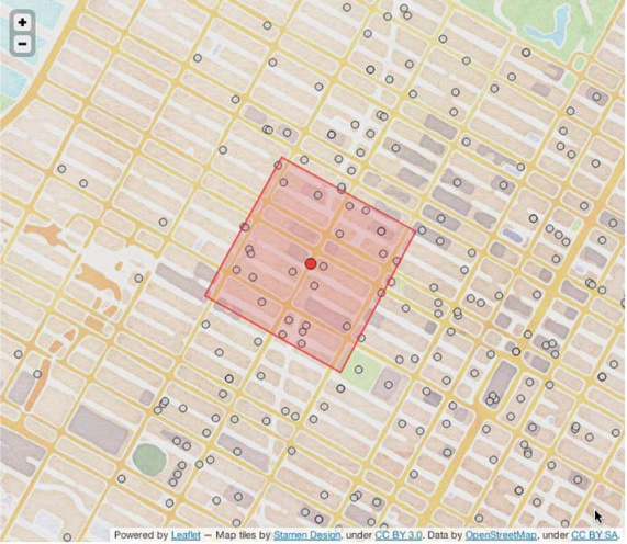
Figure 8.12 illustrates the query polygon with its centroid.
Figure 8.12. Query polygon with centroid. The centroid point is where you’ll begin with the calculation for a minimum bounding set of geohashes.
Now that you know the query polygon’s centroid, you have a place to begin calculating the geohash. The problem is, you don’t know how large a geohash is required to fully contain the query polygon. You need a way to compute a geohash and see if it fully contains the user’s query. The Geometry class in JTS has a contains() method that does just that. You also don’t want to step down the precision level if you don’t have to. If the geohash at the current precision doesn’t contain the query geometry, you should try the geohash plus all its immediate neighbors. Thus, you need a way to convert a GeoHash or a group of GeoHashes into a Geometry. This brings you to our second geometry trick: the convex hull.
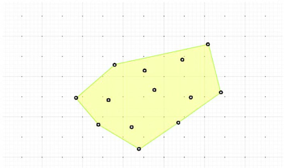
The convex hull is formally defined in terms of the intersections of sets of geometries. The Wikipedia page[16] has a simpler description that is adequate for your needs. It says you can think of the convex hull of a collection of geometries as the shape a rubber band makes when you stretch it over the geometries. These geometric concepts are easily explained in pictures, so figure 8.13[17] shows the convex hull over a random scattering of points.
16 You can find the formal definition of the convex hull at http://en.wikipedia.org/wiki/Convex_hull.
17 JTS comes with an application for exploring the interactions between geometries, called the JTSTestBuilder. This figure was created in part using that tool.
Figure 8.13. The convex hull is the shape made by fully containing a collection of geometries. In this case, the geometries are simple points. You’ll use this to test query containment of the full set of neighbors of a geohash.
The convex hull is useful for the case when you want to know if the query polygon falls inside the full set of geohash neighbors. In this case, that means whether you have a single geohash or a group of them, you can create your containment-testing polygon by taking the convex hull over the corner points from all the hashes. Every GeoHash has a BoundingBox that describes its corners. Let’s wrap that up in a method:
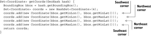
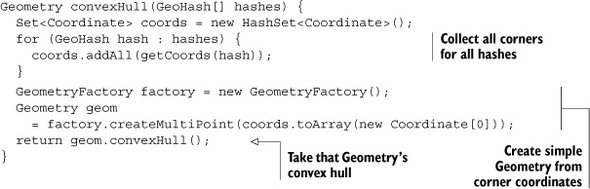
In the case of the full set of neighbors, you loop though all of them, calling getCoords() on each one, and collect their corners. Using the Coordinates, you can create a simple kind of Geometry instance, the MultiPoint. MultiPoint extends Geometry and is a group of points. You’re using this instead of something like a Polygon because the Multipoint doesn’t impose additional geometric restrictions. Create the MultiPoint and then take its convexHull(). You can put all this together in another helper method:
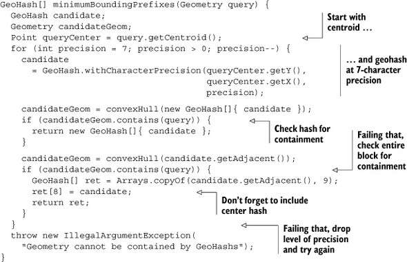
Now you have everything you need to calculate the minimum bounding set of geo-hash prefixes from the query polygon. Thus far, you’ve used a geohash precision of seven characters with reasonable success on this dataset, so you’ll start there. For this algorithm, you’ll begin by calculating the geohash at seven characters from the query polygon’s centroid. You’ll check that hash for containment. If it’s not big enough, you’ll perform the same calculation over the complete set of the geohash and its neighbors. If that set of prefixes still isn’t large enough, you’ll step the precision level back to six and try the whole thing again.
Code speaks louder than words. The minimumBoundingPrefixes() method looks like this:
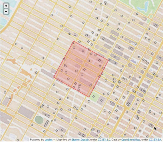
Of course, pictures speak louder than code. Figure 8.14 illustrates the attempt to bind the query with geohashes at seven and six characters of precision. Seven characters is insufficient, so a level of precision must be dropped.
Figure 8.14. Checking for containment at seven and six characters of precision. At seven characters, both the central geohash and the combined set of all its neighbors aren’t sufficiently large to cover the entire query extent. Moving up to six characters gets the job done.
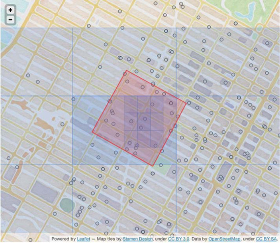
Figure 8.14 also emphasizes the imperfection in the current approach. At six-character precision, you do cover the entire query extent, but the entire western set of panels isn’t contributing any data that falls inside the query. You could be smarter in choosing your prefix panels, but that involves much more complex logic. We’ll call this good enough for now and move on to continue implementing the query.
8.4.2. Within query take 1: client side
Before building out the server-side filter, let’s finish building and testing the query logic on the client side. Deploying, testing, and redeploying any server-side component can be annoying, even when running locally, so let’s build and test the core logic client-side first. Not only that, but you’ll build it in a way that’s reusable for other kinds of queries.
The main body of client-side logic is nearly identical to that of KNNQuery. In both cases, you’re building a list of geohash prefixes to scan, running the scan, and collecting results. Because it’s largely identical, we’ll skip the scanner code. What you’re interested in is checking to see if a returned point is inside of the query polygon. To do that, you’ll need to create a Geometry instance from each QueryMatch instance. From there, the same contains() call you used earlier will do the trick:
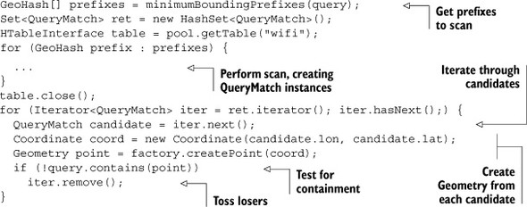
The QueryMatch results contain latitude and longitude values, so you turn those into a Coordinate instance. That Coordinate is translated into a Point, a subclass of Geometry, using the same GeometryFactory class you used earlier. contains() is just one of many spatial predicates[18] available to you via the Geometry class. That’s good news, because it means the harness you’ve built to support this within query will work for many other kinds of spatial operations.
18 If you’re curious about the full breadth of spatial predicates, check out slide 5 in this deck: Martin Davis, “JTS Topology Suite: A Library for Geometry Processing,” March 2011, http://mng.bz/ofve.
Let’s package up the code and try the query. Again, the main() method isn’t terribly interesting, just parsing arguments and dispatching the query, so you’ll skip listing it. The data is already loaded so you can get right to running the code. Rebuild and then run a query over the target area around Times Square:
$ mvn clean package
...
[INFO] -----------------------------------------------------
[INFO] BUILD SUCCESS
[INFO] -----------------------------------------------------
$ java -cp target/hbaseia-gis-1.0.0.jar
  HBaseIA.GIS.WithinQuery local
  "POLYGON ((-73.980844 40.758703,
             -73.987214 40.761369,
             -73.990839 40.756400,
             -73.984422 40.753642,
             -73.980844 40.758703))"
Geometry predicate filtered 155 points.
Query matched 26 points.
<QueryMatch:  644, dr5ru7tt72wm, -73.9852, 40.7574, NaN >
<QueryMatch:  634, dr5rukjkhsd0, -73.9855, 40.7600, NaN >
<QueryMatch:  847, dr5ru7q2tn3k, -73.9841, 40.7553, NaN >
<QueryMatch: 1294, dr5ru7hpn094, -73.9872, 40.7550, NaN >
<QueryMatch:  569, dr5ru7rxeqn2, -73.9825, 40.7565, NaN >
<QueryMatch:  732, dr5ru7fvm5jh, -73.9889, 40.7588, NaN >
<QueryMatch:  580, dr5rukn9brrk, -73.9840, 40.7596, NaN >
<QueryMatch:  445, dr5ru7zsemkp, -73.9825, 40.7587, NaN >
<QueryMatch:  517, dr5ru7yhj0n3, -73.9845, 40.7586, NaN >
<QueryMatch:  372, dr5ru7m0bm8m, -73.9860, 40.7553, NaN >
<QueryMatch:  516, dr5rue8nk1y4, -73.9818, 40.7576, NaN >
<QueryMatch:  514, dr5ru77myu3f, -73.9882, 40.7562, NaN >
<QueryMatch:  566, dr5rukk42vj7, -73.9874, 40.7611, NaN >
<QueryMatch:  656, dr5ru7e5hcp5, -73.9886, 40.7571, NaN >
<QueryMatch:  640, dr5rukhnyc3x, -73.9871, 40.7604, NaN >
<QueryMatch:  653, dr5ru7epfg17, -73.9887, 40.7579, NaN >
<QueryMatch:  570, dr5ru7fvdecd, -73.9890, 40.7589, NaN >
<QueryMatch: 1313, dr5ru7k6h9ub, -73.9869, 40.7555, NaN >
<QueryMatch:  403, dr5ru7hv4vyw, -73.9863, 40.7547, NaN >
<QueryMatch:  750, dr5ru7ss0bu1, -73.9867, 40.7572, NaN >
<QueryMatch:  515, dr5ru7g0bgy5, -73.9888, 40.7581, NaN >
<QueryMatch:  669, dr5ru7hzsnz1, -73.9862, 40.7551, NaN >
<QueryMatch:  631, dr5ru7t33776, -73.9857, 40.7568, NaN >
<QueryMatch:  637, dr5ru7xxuccw, -73.9824, 40.7579, NaN >
<QueryMatch: 1337, dr5ru7dsdf6g, -73.9894, 40.7573, NaN >
<QueryMatch:  565, dr5rukp0fp9v, -73.9832, 40.7594, NaN >
You get 26 results. That’s pretty close to our guess earlier. For a taste of things to come, notice how many points were excluded by the contains() predicate. By pushing the filter logic into the cluster, you can reduce the amount of data transmitted over the network by about 500%! First, though, let’s double-check that the results are correct. QueryMatch lines are interesting, but it’ll be easier to notice a bug if you can see the results. Figure 8.15 illustrates the query results in context of the query.
Figure 8.15. Within query results. The containment filter appears to work as expected. It’s also good to know that the geometry library appears to agree with the cartography library.
That looks pretty good. It also looks like you might want to expand the borders of the query a little. That way, it will catch the handful of locations that sit just outside the line. Now that you know the logic works, let’s push the work out to those lazy RegionServers.
8.4.3. Within query take 2: WithinFilter
Now that you have a working implementation, let’s move the predicate logic into a filter. That way you can keep all the extra data on the cluster. You have everything in place to verify the implementation via the client-side version. The only difference you should see is that the filtered version will have drastically reduced network overhead and thus, ideally, run faster. Unless, that is, you’re running against a dataset on a standalone HBase.
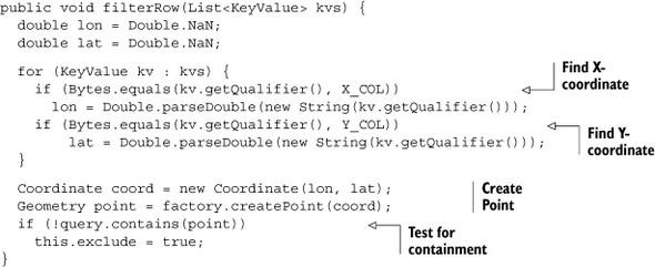
The WithinFilter is similar to the PasswordStrengthFilter you saw in chapter 4. Just like PasswordStrengthFilter, you’re filtering based on data stored in the cells within the row, so you need to maintain some state. In this case, you need to override the void filterRow(List<KeyValue>) method in order to access both the X- and Y-coordinates at the same time. That’s where you’ll move the logic from the client-side implementation. That method will update the state variable in the cases when you want to exclude a row. Minus a little error-checking, the filterRow() method looks like this:
Methods that iterate over every KeyValue in every column family in every row can be slow. HBase will optimize away calls to filterRow() if it can; you must explicitly enable it in your extension to FilterBase. Tell the filter to tell HBase to call this method by providing one more override:
public boolean hasFilterRow() { return true; }
When you want to exclude a row because it doesn’t fall within the query bounds, you set the exclude flag. That flag is used in boolean filterRow() as the condition for exclusion:
public boolean filterRow() {
  return this.exclude;
}
You’ll construct your filter from the query Geometry parsed from main()’s arguments. Constructing the filter on the client looks like this:
Filter withinFilter = new WithinFilter(query);
Other than moving the exclusion logic out to the Filter implementation, the updated method doesn’t look very different. In your own filters, don’t forget to include a default constructor with no arguments. That’s necessary for the serialization API. Now it’s time to install the filter and give it a go.
At the time of this writing, there aren’t many examples of custom Filter implementations. We have the list of filters that ship with HBase (an impressive list) but not much beyond that. Thus if you choose to implement your own filters, you may find yourself scratching your head. But never fear! HBase is open, and you have the source!
If you think HBase isn’t respecting a contract between the interface and its calling context, you can always fall back to the source. A handy trick for such things is to create and log an exception. There’s no need to throw it; just create it and log it. LOG.info("", new Exception()); should do the trick. The stack trace will show up in your application logs, and you’ll know exactly where to dive into the upstream code. Sprinkle exceptions throughout to get a nice sampling of what is (or isn’t) calling your custom filter.
If you’re debugging a misbehaving filter, you’ll have to stop and start HBase with each iteration so it picks up the changes to your JAR. That’s why in the example, you tested the logic on the client side first.
The filter must be installed on the HBase cluster in order for your RegionServers to be able to instantiate it. Add the JAR to the classpath, and bounce the process. If your JAR includes dependencies as this one does, be sure to register those classes as well. You can add those JARs to the classpath, or you can create an uber-JAR, exploding all of those JARs’ classes inside your own. That’s what you do here, for simplicity. In practice, we recommend that you keep your JAR lean and ship the dependencies just as you do your own. It will simplify debugging the version conflicts that will inevitably pop up later down the line. Your future self will thank you. The same applies to custom Coprocessor deployments.
To find out exactly which external JARs your Filter or Coprocessor depends on, and which JARs those dependencies depend on, Maven can help. It has a goal for determining exactly that. In this case, it shows only two dependencies not already provided by Hadoop and HBase:
$ mvn dependency:tree
...
[INFO] --- maven-dependency-plugin:2.1:tree (default-cli) @ hbaseia-gis ---
[INFO] HBaseIA:hbaseia-gis:jar:1.0.0-SNAPSHOT
[INFO] +- org.apache.hadoop:hadoop-core:jar:1.0.3:compile
[INFO] |  +- commons-cli:commons-cli:jar:1.2:compile
...
[INFO] +- org.apache.hbase:hbase:jar:0.92.1:compile
[INFO] |  +- com.google.guava:guava:jar:r09:compile
...
[INFO] +- org.clojars.ndimiduk:geohash-java:jar:1.0.6:compile
[INFO] - com.vividsolutions:jts:jar:1.12:compile
[INFO] ------------------------------------------------------------------
[INFO] BUILD SUCCESS
[INFO] ------------------------------------------------------------------
You’re lucky: the dependencies don’t pull any dependencies of their own—at least, no JARs not already provided. Were there any, they’d show up in the tree view.
You install the JAR and any dependencies by editing the file hbase-env.sh in $HBASE_HOME/conf. Uncomment the line that starts with export HBASE_CLASSPATH, and add your JAR. You can add multiple JARs by separating them with a colon (:). It looks something like this:
# Extra Java CLASSPATH elements.  Optional.
export HBASE_CLASSPATH=/path/to/hbaseia-gis-1.0.0.jar
Now you can rebuild, restart, and try it. Notice that you change the first parameter of the query tool’s launch command from local to remote:
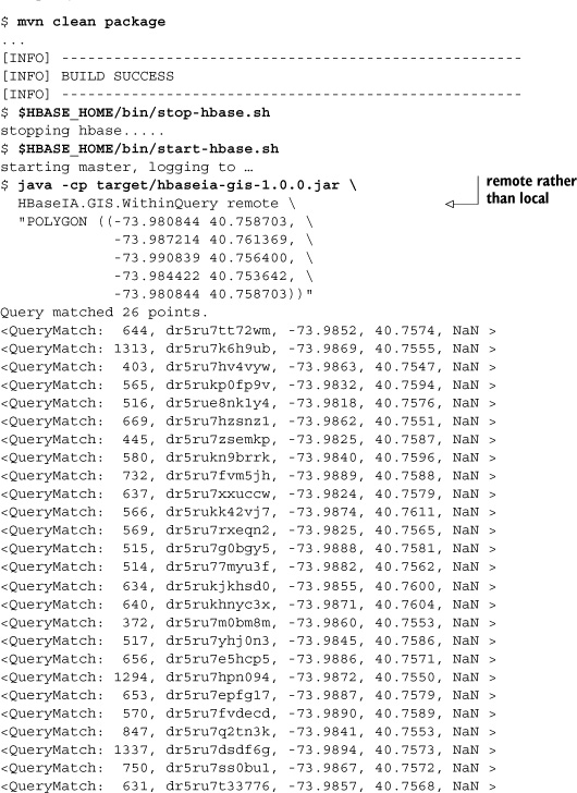
The same number of points are returned. A quick cat, cut, sort, diff will prove the output is identical. Visual inspection via figure 8.16 confirms this.
Figure 8.16. Results of the filtered scan. This should look an awful lot like figure 8.15.

The final test would be to load lots of data on a distributed cluster and time the two implementations. Queries over a large area will show significant performance gains. Be careful, though. If your queries are really big, or you build up a complex filter hierarchy, you may run into RPC timeouts and the like. Refer to our previous comments about setting scanner caching (section 8.3) to help mitigate that.
8.5. Summary
This chapter was as much about GIS as about HBase. Remember, HBase is just a tool. To use it effectively, you need to know both the tool and the domain in which you want to apply it. The geohash trick proves that point. A little domain knowledge can go a long way. This chapter showed you how to combine that domain knowledge with your understanding of HBase to create an efficient tool for churning through mounds of GIS data efficiently and in parallel. It also showed you how to push application logic server-side and provided advice on when and why that might be a good idea.
It’s also worth noting that these queries are only the beginning. The same techniques can be used to implement a number of other spatial predicates. It’s no replacement for PostGIS,[19] but it’s a start. It’s also only the beginning of exploring how to implement these kinds of multidimensional queries on top of HBase. As an interesting follow-up, a paper was published in 2011[20] that explores methods for porting traditional data structures like quad-trees and kd-trees to HBase in the form of a secondary index.
19 PostGIS is a set of extensions to the PostgreSQL database and is the canonical open source GIS database in the open source world. If you thought the geohash algorithm was clever, peek under the hood of this system: http://postgis.refractions.net/.
20 Shoji Nishimura, Sudipto Das, Divyakant Agrawal, and Amr El Abbadi, “MD-HBase: A Scalable Multidimensional Data Infrastructure for Location Aware Services,” 2011, www.cs.ucsb.edu/~sudipto/papers/md-hbase.pdf.
This chapter concludes the portion of this book dedicated to building applications on HBase. Don’t think the book is over, though. Once your code is written and your JARs ship, the fun has only begun. From here on out, you’ll get a sense of what it takes to plan an HBase deployment and how to run HBase in production. Whether you’re working on the project plan as a project manager or a network administrator, we hope you’ll find what you need to get started. Application developers will find the material useful as well. Your application’s performance depends quite a bit on configuring the client to match your cluster configuration. And of course, the more you know about how the cluster works, the better equipped you are to solve production bugs in your application.