
Structural Breaks, Efficiency, and Volatility: An Empirical Investigation of Southeast Asian Frontier Markets
Abstract
The purpose of this study is to examine the presence of structural breaks, efficiency, and volatility in the frontier markets of Southeast Asia. Using daily and weekly returns of four composite indices (VN Index, HNX Index, LSX Index, and CSX Index), we measure the presence of price volatility in the markets of Vietnam, Laos, and Cambodia. Our findings from all tests—unit root, autocorrelation, run, and variance ratio—suggest that the Vietnamese stock market is weak-form inefficient, while in the cases of Laos and Cambodia the empirical statistics produce inconclusive results. Furthermore, symmetric volatility models are statistically significant in both daily and weekly series, implying that the impacts of positive and negative news or shocks are the same in magnitude.
Keywords
1. Introduction
2. Literature Review
3. Data and Methodology
3.1. The Data
Table 13.1
Summary of Sample Size for the Index of Each SEA Frontier Stock Market
| Index | Frontier market | Sample period | No. of daily observations | No. of weekly observations |
| VN Index | Vietnam | Jul. 28, 2000 to Dec. 31, 2014 | 3432 | 741 |
| HNX Index | Vietnam | Jan. 4, 2006 to Dec. 31, 2014 | 2194 | 462 |
| LSX Index | Lao PDR | Jan. 12, 2011 to Dec. 31, 2014 | 983 | 170 |
| CSX Index | Cambodia | Apr. 19, 2012 to Dec. 31, 2014 | 616 | 141 |

 (13.1)
3.2. Tests for Randomness
 (13.3)
 (13.4)
 (13.5)
 (13.6)
 (13.7)
 (13.9)
 ). Similarly, we calculate
 (13.10)
 (13.11)
 (13.12)
 ,
, 3.3. Structural Breaks, Long Memory Dynamics, and Test for Volatility
 (13.14)
 (13.15)
 (13.17)
 should be less than unity to satisfy stationarity conditions. If βj are all zero, the equation reduces to the ARCH(p) process described in Eq. 13.16—the earliest form of the volatility model developed by Engle (1982). It is rare for the order (p, q) of a GARCH model to be high, while a GARCH(p, q) can be extended to allow for the inclusion of exogenous or predetermined regressors (z) in the variance equation, mathematically notated as
 (13.18)
 (13.19)
4. Empirical Results
4.1. Results From Randomness Tests
Table 13.2
Unit Root Test Results for the Index of Each SEA Frontier Stock Market
| Panel A: daily returns | ||||
| Index | VN Index | HNX Index | LSX Index | CSX Index |
| Intercept | −21.103*** | −38.943*** | −16.344*** | −23.526*** |
| Intercept, linear trend | −21.126*** | −38.949*** | −16.337*** | −23.568*** |
| None | −21.076*** | −38.952*** | −16.346*** | −23.311*** |
| Panel B: weekly returns | ||||
| Index | VN Index | HNX Index | LSX Index | CSX Index |
| Intercept | −15.347*** | −17.273*** | −10.354*** | −11.071*** |
| Intercept, linear trend | −15.367*** | −17.281*** | −10.363*** | −11.010*** |
| None | −15.316*** | −17.292*** | −10.402*** | −10.930*** |

Notes: The VN Index represents large-cap stocks (>VND 120 billion), while the HNX Index consists of medium and small-cap companies listed on the Vietnamese stock exchange. The LSX Index and the CSX Index are the composite indices of the Laos Securities Exchange and the Cambodia Stock Exchange, respectively. *** signifies the rejection of the null hypothesis of having a unit root at a 1% level of significance.
Table 13.3
Autocorrelation Test Results for Daily SEA Frontier Stock Market Indices
| Panel A: daily returns | ||||||||
| Index | VN Index | HNX Index | LSX Index | CSX Index | ||||
| Lag | AC | Q-stat | AC | Q-stat | AC | Q-stat | AC | Q-stat |
| 1 | 0.30 | 308.51*** | 0.18 | 72.16*** | 0.18 | 30.80*** | 0.056 | 1.92 |
| 3 | 0.02 | 318.70*** | 0.04 | 77.36*** | 0.04 | 39.85*** | 0.017 | 3.52 |
| 5 | 0.12 | 395.94*** | 0.07 | 101.01*** | 0.09 | 52.20*** | 0.071 | 6.84 |
| 7 | 0.05 | 430.39*** | −0.01 | 101.30*** | 0.02 | 58.16*** | 0.003 | 7.35 |
| 9 | 0.03 | 436.23*** | 0.05 | 109.57*** | 0.04 | 68.00*** | −0.009 | 7.52 |
| 11 | 0.05 | 451.55*** | 0.02 | 110.60*** | 0.03 | 70.09*** | 0.082 | 12.62 |
| 13 | 0.04 | 458.43*** | 0.04 | 115.25*** | −0.03 | 70.99*** | 0.024 | 18.42 |
| 15 | 0.06 | 487.26*** | 0.01 | 120.39*** | −0.08 | 80.12*** | 0.055 | 20.35 |
| Panel B: weekly returns | ||||||||
| Index | VN Index | HNX Index | LSX Index | CSX Index | ||||
| Lag | AC | Q-stat | AC | Q-stat | AC | Q-stat | AC | Q-stat |
| 1 | 0.16 | 20.07*** | 0.21 | 20.61*** | 0.35 | 21.32*** | 0.16 | 3.86** |
| 3 | 0.11 | 47.56*** | 0.09 | 28.63*** | −0.08 | 22.57*** | −0.03 | 4.56 |
| 5 | 0.16 | 71.56*** | 0.06 | 36.77*** | −0.09 | 24.53*** | 0.11 | 6.82 |
| 7 | 0.07 | 76.29*** | 0.06 | 39.47*** | 0.01 | 25.19*** | −0.04 | 7.05 |
| 9 | 0.06 | 78.91*** | 0.03 | 39.82*** | 0.03 | 25.53*** | −0.08 | 8.18 |
| 11 | 0.00 | 79.14*** | −0.01 | 39.89*** | 0.07 | 26.90*** | 0.02 | 8.53 |
| 13 | −0.02 | 80.12*** | −0.04 | 41.81*** | 0.04 | 28.47*** | −0.06 | 11.04 |
| 15 | −0.11 | 88.63*** | −0.07 | 45.34*** | −0.04 | 28.92** | 0.02 | 11.29 |

Notes: The VN Index represents large-cap stocks (>VND 120 billion), while the HNX Index consists of medium and small-cap companies listed on the Vietnamese stock exchange. The LSX Index and the CSX Index are the composite indices of the Laos Securities Exchange and the Cambodia Stock Exchange, respectively. *** and ** signify the rejection of the null hypothesis of no autocorrelation at the 1 and 5% levels of significance, respectively.
Table 13.4
Runs Test Results for Daily SEA Frontier Stock Market Indices
| Panel A: daily returns | ||||
| Index | VN Index | HNX Index | LSX Index | CSX Index |
| E(R) | 1715.765 | 1097.482 | 473.230 | 259.699 |
| var(R) | 856.7655 | 547.981 | 226.839 | 108.577 |
| StDev(R) | 29.271 | 23.409 | 15.061 | 10.420 |
| Z-stat | −11.984*** | −4.677*** | −0.480 | −2.178** |
| Panel B: weekly returns | ||||
| Index | VN Index | HNX Index | LSX Index | CSX Index |
| E(R) | 370.903 | 231.499 | 82.657 | 68.586 |
| var(R) | 184.652 | 114.998 | 39.203 | 32.376 |
| StDev(R) | 13.589 | 10.724 | 6.261 | 5.689 |
| Z-stat | −4.703*** | −3.497*** | −0.424 | −0.454 |

Notes: The VN Index represents large-cap stocks (>VND 120 billion), while the HNX Index consists of medium and small-cap companies listed in the Vietnamese stock exchange. The LSX Index and the CSX Index are the composite indices of the Laos Securities Exchange and the Cambodia Stock Exchange, respectively. *** signifies the rejection of the null hypothesis of no autocorrelation at a 1% level of significance.
Table 13.5
Variance Ratio Test Results for Daily SEA Frontier Stock Market Indices
| Panel A: daily returns | ||||
| Index | VN Index | HNX Index | LSX Index | CSX Index |
| Ranks | 19.032*** | 17.737*** | 14.533*** | 11.606*** |
| Rank scores | 20.559*** | 18.765*** | 14.701*** | 12.246*** |
| Signs | 12.943*** | 12.944*** | 10.313*** | 8.297 |
| Panel B: weekly returns | ||||
| Index | VN Index | HNX Index | LSX Index | CSX Index |
| Ranks | 11.636*** | 8.484*** | 5.574*** | 4.953*** |
| Rank scores | 12.708*** | 8.889*** | 5.421*** | 5.467*** |
| Signs | 7.982*** | 5.875*** | 4.320*** | 2.799** |

Notes: The VN Index represents large-cap stocks (>VND 120 billion), while the HNX Index consists of medium and small-cap companies listed in the Vietnamese stock exchange. The LSX Index and the CSX Index are the composite indices of the Laos Securities Exchange and the Cambodia Stock Exchange, respectively. *** and ** signify the rejection of the null hypothesis of random walk at the 1 and 5% levels of significance, respectively.
4.2. Results on Structural Breaks and Volatility
Table 13.6
Bai-Perron (2003) Structural Break Test Results
| Panel A: daily returns | |||||
| Country | Global L breaks versus none | ||||
| F-stat and scaled F-stat | Weighted F-stat | UDMax stat** | WDMax stat** | Break dates | |
| VN Index | 6.635 4.983 5.275 |
6.635 5.922 7.594 |
6.635 | 7.594 | Oct. 27, 2003 Feb. 28, 2007 Jan. 4, 2009 |
| HNX Index | 5.592 4.816 4.063 |
5.592 5.723 5.849 |
5.592 | 5.849 | Oct. 17, 2007 Feb. 25, 2009 Jun. 17, 2010 |
| LSX Index | 0.352 3.467 2.981 |
0.352 4.120 4.291 |
3.467 | 4.291 | Feb. 20, 2012 Jan. 22, 2013 Jan. 27, 2014 |
| CSX Index | 1.857 3.427 2.031 |
1.857 4.072 2.924 |
4.073 | 3.427 | Mar. 16, 2012 Mar. 22, 2013 Feb. 08, 2014 |
| Panel B: weekly returns | |||||
| Country | Global L breaks versus none | ||||
| F-stat and scaled F-stat | Weighted F-stat | UDMax stat** | WDMax stat** | Break dates | |
| VN Index | 5.972 4.185 4.17 |
5.972 4.973 5.927 |
5.972 | 5.972 | Oct. 17, 2003 Jan. 19, 2007 Mar. 6, 2009 |
| HNX Index | 4.434 3.956 3.215 |
4.434 4.698 4.629 |
4.434 | 4.698 | Oct. 19, 2007 Feb. 13, 2009 Jun. 18, 2010 |
| LSX Index | 0.684 3.147 4.164 |
0.685 3.740 5.995 |
4.164 | 5.995 | Jul. 22, 2011 Jan. 27, 2012 Feb. 1, 2013 |
| CSX Index | 2.922 3.049 2.002 |
2.922 3.623 2.882 |
3.049 | 3.624 | Sep. 21, 2012 May 31, 2013 Oct. 25, 2013 |

Notes: The VN Index represents large-cap stocks (>VND 120 billion), while the HNX Index consists of medium and small-cap companies listed in the Vietnamese stock exchange. The LSX Index and the CSX Index are the composite indices of the Laos Securities Exchange and the Cambodia Stock Exchange, respectively.
Table 13.7
Results From Volatility Models (Daily Returns)
| Panel A: mean equation | |||
| VN Index | AR(1) | MA(1) | MA(2) |
ARIMA(1,0,2)(0,0,0) z-statistic |
0.994 452.870*** |
−0.745 −39.238*** |
−0.237 −12.513*** |
| HNX Index | AR(1) | MA(1) | |
ARIMA(1,0,1)(0,0,0) z-statistic |
0.669 5.989*** |
−0.556 −4.648*** |
|
| LSX Index | AR(1) | MA(1) | |
ARIMA(1,0,1)(0,0,0) z-statistic |
0.869 22.023*** |
−0.887 −26.312*** |
|
| CSX Index | AR(1) | MA(1) | |
ARIMA(1,0,1)(0,0,0) z-statistic |
0.957 52.092*** |
−0.982 −102.824*** |
|
| Panel B: conditional variance equations | ||||
| ω | α1 | β1 | D2 | |
| VN Index | ||||
EGARCH (1,1) z-statistic |
−0.789 −10.493*** LL = 10,329.73 |
0.434 14.101*** SBC = −6.007 |
0.949 131.426*** QSQ(12) = 32.192 (0.650) |
0.263 2.320** |
| HNX Index | ||||
EGARCH (1,1) z-statistic |
−0.651 −7.235*** LL = 5,688.361 |
0.397 10.995*** SBC = −5.173 |
0.956 102.933*** QSQ(12) = 4.616 (0.948) |
|
| LSX Index | ||||
EGARCH (1,1) z-statistic |
0.000 3.861*** LL = 3,036.301 |
0.361 5.524*** SBC = −6.155 |
0.373 3.531*** QSQ(12) = 26.065 (0.889) |
|
| CSX Index | ||||
EGARCH (1,1) z-statistic |
−1.293 −2.970*** LL = 1,828.873 |
0.370 4.519*** SBC = −5.941 |
0.879 19.312*** QSQ(12) = 40.825 (0.267) |
|

Notes: The VN Index represents large-cap stocks (>VND 120 billion), while the HNX Index consists of medium and small-cap companies listed in the Vietnamese stock exchange. The LSX Index and the CSX Index are the composite indices of the Laos Securities Exchange and the Cambodia Stock Exchange, respectively. *D2 is a dummy variable representing structural breaks. *** and ** signify the rejection of the null hypothesis of random walk at the 1 and 5% levels of significance, respectively.
Table 13.8
Results From Volatility Models (Weekly Returns)
| Panel A: mean equation | ||||
| VN Index | AR(1) | AR(2) | MA(1) | MA(2) |
ARIMA(2,0,2)(0,0,0) z-statistic |
−0.360 −2.303** |
−2.303 4.028*** |
0.520 2.944*** |
−0.455 −2.624*** |
| HNX Index | AR(1) | MA(1) | ||
ARIMA(1,0,1)(0,0,0) z-statistic |
0.669 5.990*** |
−0.556 −4.648*** |
||
| LSX Index | AR(1) | MA(1) | ||
ARIMA(1,0,1)(0,0,0) z-statistic |
−0.943 −63.156*** |
0.983 223.576*** |
||
| CSX Index | AR(1) | MA(1) | ||
ARIMA(1,0,1)(0,0,0) z-statistic |
0.544 2.540** |
−0.530 −2.678** |
||
| Panel B: conditional variance equations | ||||||
| ω | α1 | β1 | D1 | D2 | D3 | |
| VN Index | ||||||
EGARCH (1,1) |
−0.585 −4.101*** |
0.407 5.625*** |
0.959 62.687*** |
0.685 3.075*** |
−0.455 −2.624*** |
|
| z-statistic | LL = 1426.6 | SBC = −3.8 | QSQ(12) = 27.2 (0.854) |
|||
| HNX Index | ||||||
| EGARCH (1,0) | −6.259 −46.159*** |
0.360 4.193*** |
−5.021 −15.582*** |
1.283 3.968*** |
||
| z-statistic | LL = 725.3 | SBC = −3.1 | QSQ(12) = 19.8 (0.975) | |||
| LSX Index | ||||||
| EGARCH (1,1) | −0.557 −5.24*** |
−0.409 −5.460*** |
0.891 68.347*** |
|||
| z-statistic | LL = 407.3 | SBC = −4.7 | QSQ(12) = 45.8 (0.128) | |||
| CSX Index | ||||||
| EGARCH (1,0) | −7.530 −28.748*** |
0.517 2.541** |
−1.383 −2.362** |
−4.494 −9.045*** |
1.641 2.438** |
|
| z-statistic | LL = 310.1 | SBC = −4.2 | QSQ(12) = 10.3 (0.999) |
|||
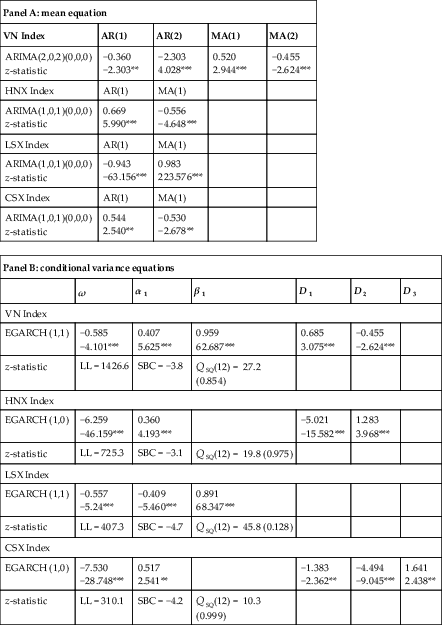
Notes: The VN Index represents large-cap stocks (>VND 120 billion), while the HNX Index consists of medium and small-cap companies listed in the Vietnamese stock exchange. The LSX Index and the CSX Index are the composite indices of the Laos Securities Exchange and the Cambodia Stock Exchange, respectively.
* D1, D2, and D3 are dummy variables represent the structural breaks. *** and ** signify the rejection of the null hypothesis of random walk at the 1 and 5% levels of significance, respectively.
5. Conclusions
a A time series process is characterized as stationary if its mean and variance are constant and the covariance between two different time periods depends upon the lag between them. The mean and variance of the time series are estimated as (Yt) = μ and Var(Yt) = E(Yt–μ)2, respectively. The covariance of Y values at times t and t + k is estimated as γk = E[(Yt–μ)(Yt+k–μ)], while a unit root is defined by using the first-order autoregressive model of Yt = ρYt − 1 + μt with (−1 ≤ ρ ≤ 1). If ρ = 1, there is a unit root in the time series process.
b Dickey and Fuller (1981) show that the coefficient after transformation to δ does not follow a normal distribution when the size of the sample is large. This results in conventional t-statistic results being erroneous.
c This will indicate that the variance is a linear function of the relevant holding periods.
d Wright (2000) has extended the Lo and MacKinlay test (1988) by introducing rank differences, so that the variance ratio test could be applied in cases in which the distribution of returns is not normally distributed.
e Nonetheless, prior literature suggests that in practice this βj ≥ 0 constraint can be overrestrictive (Nelson and Cao, 1992; Tsai and Chan, 2008).
f These breaks in the return time series are triggered by important political or economic events in the countries in question. For example, the structural break of Oct. 27, 2003, for Vietnam follows immediately after the signing of an agreement between the governments of Vietnam and the United States to start—for the first time since the end of the Vietnam War—commercial flights between the two countries. Meanwhile, the break of Feb. 28, 2007, is driven by the Vietnamese government’s announcement to invest US$33bn in infrastructure projects, for example, a high-speed rail link between Hanoi and Ho Chi Minh City.